Abstract

We compute the expectations of the squares of the electric and magnetic fields in the vacuum region outside a half-space filled with a uniform dispersive dielectric. We find a positive energy density of the electromagnetic field which diverges at the interface despite the inclusion of dispersion in the calculation. We also investigate the mean squared fields and the energy density in the vacuum region between two parallel half-spaces. Of particular interest is the sign of the energy density. We find that the energy density is described by two terms: a negative position independent (Casimir) term, and a positive position dependent term with a minimum value at the center of the vacuum region. We argue that in some cases, including physically realizable ones, the negative term can dominate in a given region between the two half-spaces, so the overall energy density can be negative in this region.

PACS categories: 12.20.Ds, 03.70.+k, 77.22.Ch, 04.62.+v.

1
  Introduction              

In 1948 Casimir made the remarkable prediction that there is an attractive force between a pair uncharged parallel plane perfect conductors [1]. Furthermore, he argued that this force arises solely from a shift in the energy of the vacuum state of the quantized electromagnetic field. An early attempt by Sparnaay [2] to observe this force was inconclusive, but in recent years several new experiments [3, 4, 5, 6, 7] have been performed which seem to give good agreement with Casimir’s prediction. (To be more precise, most of these experiments actually measure the force between a plate and a sphere and incorporate a theoretical correction to compare to Casimir’s result. Of the recent experiments, only that of Bressi et al [7] uses two parallel plates.)

If the energy of the vacuum state is zero in the limit of infinite plate separation, then the attractive force found by Casimir would seem to imply a negative vacuum energy at finite separation. In fact, Brown and Maclay [8] showed that for perfectly conducting plates, one has a constant negative vacuum energy density. This conclusion is of great theoretical interest, because negative energy density has the potential to cause some rather bizarre effects in gravity theory. (See, for example, Ref. [9] and references therein.) However, questions have been raised as to whether the negative energy density will still arise in a more realistic treatment in which the plates are not perfect conductors [10, 11]. In particular, Helfer and Lang [10] calculated the energy density outside of a single half-space filled with a nondispersive dielectric material and obtained a positive result. They interpreted this as a positive self-energy density associated with a single plate which would add to the negative interaction energy density between a pair of plates. Helfer and Lang conjecture that the net Casimir energy density might be positive when the self energy is accounted for. If this conjecture is correct, then the situation would be analogous to that of the energy density in classical electrostatics. A pair of oppositely charged particles have a negative interaction energy, but the net energy density, which is proportional to the square of the electric field, is always positive.

However, the Helfer and Lang calculation does not include dispersion, which is essential in a realistic treatment. Numerous authors, beginning with Lifshitz [12], have studied the effects of dispersion upon Casimir forces. However, these authors have been concerned with the force or the total energy, and not the local energy density. The purpose of this paper is to present a calculation of the Casimir energy density in a model in which dispersion is included. For this purpose, we will use the methods of source theory developed by Schwinger and coworkers [13, 14]. This is a method based upon the calculation of Green’s functions which is especially well suited to dissipative materials, and was used by Schwinger et al [13] to rederive the results of Lifshitz. Milonni and Shih [15] have used conventional quantum electrodynamics to reproduce some of the results of source theory. There has also been considerable interest in recent years in quantization of the electromagnetic field inside dissipative materials using operator methods [16, 17, 18]. The relation between the results of the latter set of authors and those of Schwinger et al has not yet been clarified.

The outline of this paper is as follows: In Sect. 2 we review the source theory approach as applied to parallel interfaces of dielectric media. In Sect. 3 we compute the expectation values of the squares of the electric and magnetic fields in the vacuum region outside a half-space filled with a uniform dispersive dielectric. We extend this calculation to the case of two parallel dielectric half-spaces and also discuss the energy density in Sect. 4. Conclusions are given in Sect. 5.

2 Green-Function Approach for Multilayer Dielectrics

This section is a review of the formalism of Schwinger et al [13]. One begins by writing the Maxwell equations for the macroscopic electromagnetic fields produced by an external polarization source $\mathbf{P}$, which formally describes the zero point fluctuations of the fields

$$\mathbf{B}=\nabla\times\mathbf{A},$$

$$\mathbf{E}=-\dot{\mathbf{A}}-\nabla\phi,$$

$$\nabla\times\mathbf{B}=\epsilon\dot{\mathbf{E}}+\dot{\mathbf{P}},$$ (1)

$$\nabla\cdot(\epsilon\mathbf{E}+\mathbf{P})=0,$$

where $\epsilon$ is the dielectric constant of the medium. The wave equation for the electric field resulting from the Maxwell equations is

$$-\nabla\times(\nabla\times\mathbf{E})-\epsilon\ddot{\mathbf{E}}=\ddot{\mathbf{P}},$$ (2)

By assuming a linear relation between sources and fields, the electric field can be written as a spacetime integral

$$\mathbf{E}(x)=\int d^{4}x^{\prime}\mathbf{\,}\overleftrightarrow{\mathbf{\Gamma}}\mathbf{(}x,x^{\prime}\mathbf{)\,\mathbf{P}(}x^{\prime}\mathbf{),}$$ (3)

where $x=(t,\mathbf{r})$, $x^{\prime}=(t^{\prime},\mathbf{r}^{\prime})$ and $\overleftrightarrow{\mathbf{\Gamma}}$ is a Green’s dyadic, which satisfies (2) with a $\delta$-function source. Let

$$\overleftrightarrow{\mathbf{\Gamma}}(\mathbf{r},\mathbf{r}^{\prime},\omega)=\int_{-\infty}^{\infty}d\tau\,e^{i\omega\tau}\,\overleftrightarrow{\mathbf{\Gamma}}(x,x^{\prime})\,,$$ (4)

where $\tau=t-t^{\prime}$. From (2) and (3), it follows that $\mathbf{\overleftrightarrow{\mathbf{\Gamma}}}(\mathbf{r},\mathbf{r}^{\prime},\omega)$ satisfies the following equation:

$$-\nabla\times(\nabla\times\mathbf{\overleftrightarrow{\mathbf{\Gamma}})+}\omega^{2}\epsilon\mathbf{\overleftrightarrow{\mathbf{\Gamma}}=-}\omega^{2}\,\mathbf{\overleftrightarrow{\mathbf{1}}}\delta\mathbf{(\mathbf{r}-\mathbf{r}^{\prime}).}$$ (5)

So far, the discussion has been purely classical. At this point, Schwinger et al [13] use source theory to identify the Green’s dyadic $\overleftrightarrow{\mathbf{\Gamma}}$ with an “effective product of electric fields”

$$\frac{i}{\hbar}\langle E_{j}(\mathbf{r})\,E_{k}(\mathbf{r}^{\prime})\rangle=\Gamma_{jk}(\mathbf{r},\mathbf{r}^{\prime},\omega).$$ (6)

We can interpret this as the Fourier transform of the electric field correlation function. From the Maxwell equation $\nabla\times\mathbf{E=-\dot{B}}$, one finds the corresponding expression for the magnetic field:

$$\frac{i}{\hbar}\langle B_{j}(\mathbf{r})\,B_{k}(\mathbf{r}^{\prime})\rangle=\epsilon_{jlm}\epsilon_{knp}(\nabla_{l}\nabla_{n^{\prime}}/\omega^{2}\,)\Gamma_{mp}(\mathbf{r},\mathbf{r}^{\prime},\omega).$$ (7)

Note that $\hbar$ makes its first appearance in these expressions. These expressions can be identified with the vacuum expectation values of products of field operators, which appear in the more conventional field theory approach to quantization of the electromagnetic field. From now onward, we revert to units in which $\hbar=1$. In order to calculate the field correlation functions, one needs to find the Green’s function $\mathbf{\Gamma}$ occurring in (5). This amounts to solving a classical boundary value problem.

The interfaces between the media are chosen to be perpendicular to the $z$ direction, so for now it will only matter that the dielectric constant changes in the $z$ direction only. Therefore, it is convenient to introduce a transverse spatial Fourier transform

$$\mathbf{\overleftrightarrow{\mathbf{\Gamma}}(\mathbf{r},\mathbf{r}^{\prime},}\omega\mathbf{)=\int}d\mathbf{\mathbf{k}_{\bot}\;}\frac{1}{(2\pi)^{2}}e^{i\mathbf{k}_{\bot}(\mathbf{r}-\mathbf{r}^{\prime})_{\bot}}\mathbf{\overleftrightarrow{\mathbf{\Gamma}}(}z,z^{\prime}\mathbf{,\mathbf{k}_{\bot},}\omega\mathbf{),}$$ (8)

where the vector $\mathbf{k}_{\perp}$ can be chosen to point along the $+x$ axis ($k=\left|\mathbf{k}_{\perp}\right|$).

Some components of $\mathbf{\overleftrightarrow{\mathbf{\Gamma}}}$are found to be [13]

$$\Gamma_{xx} = -\frac{1}{\epsilon}\delta(z-z^{\prime})+\frac{1}{\epsilon}\frac{\partial}{\partial z}\frac{1}{\epsilon^{\prime}}\frac{\partial}{\partial z^{\prime}}g^{B},$$ (9a)

$$\Gamma_{yy} = \omega^{2}g^{E},$$ (9b)

$$\Gamma_{zz} = -\frac{1}{\epsilon}\delta(z-z^{\prime})+\frac{k^{2}}{\epsilon\epsilon^{\prime}}g^{B},$$ (9c)

$$\Gamma_{xz} = i\frac{k}{\epsilon\epsilon^{\prime}}\frac{\partial}{\partial z}g^{B},$$ (9d)

$$\Gamma_{zx} = -i\frac{k}{\epsilon\epsilon^{\prime}}\frac{\partial}{\partial z^{\prime}}g^{B},$$ (9e)

where $\epsilon^{\prime}=\epsilon(z^{\prime})$, and $g^{E}$, the “transverse electric”, and $g^{B}$, the “transverse magnetic” Green’s functions satisfy

$$\left[-\frac{\partial^{2}}{\partial z^{2}}+k^{2}-\omega^{2}\epsilon\right]g^{E}(z,z^{\prime}) = \delta(z-z^{\prime}),$$ (10a)

$$\left[-\frac{\partial}{\partial z}\frac{1}{\epsilon}\frac{\partial}{\partial z}+\frac{k^{2}}{\epsilon}-\omega^{2}\right]g^{B}(z,z^{\prime}) = \delta(z-z^{\prime}).$$ (10b)

By introducing the quantity

$$\kappa^{2}=k^{2}-\omega^{2}\epsilon,$$ (11)

(2) can be written as:

$$\left[-\frac{\partial^{2}}{\partial z^{2}}+\kappa^{2}\right]g^{E}(z,z^{{}^{\prime}}) = \delta(z-z^{\prime}),$$ (12a)

$$\left[-\frac{\partial}{\partial z}\frac{1}{\epsilon}\frac{\partial}{\partial z}+\frac{\kappa^{2}}{\epsilon}\right]g^{B}(z,z^{\prime}) = \delta(z-z^{\prime}).$$ (12b)

So, in order to find the field correlation functions as defined in (6) and (7) in a given situation, one needs to solve these equations with the appropriate boundary conditions. We consider here two cases.

3 One Interface Case

We now specialize the above discussion to a situation in which the inhomogeneity of the dielectric constant is due to a plane interface separating a dielectric substance from a vacuum:

$$z>0:\,\,\epsilon(z) = 1,$$

$$z<0:\,\,\epsilon(z) \equiv \epsilon_{d}.$$ (13)

Here $\epsilon_{d}$ is a function of frequency, but not of position.

3.1 Boundary Conditions

In solving (12a) and (12b), we use the following boundary conditions. At $z=z^{\prime}$, $g$ is continuous but the derivative is discontinuous at this point [19]:

$$\frac{\partial g}{\partial z}\biggl{|}_{z\rightarrow z_{-}^{\prime}}^{z\rightarrow z_{+}^{\prime}}=-1.$$ (14)

At the boundary ($z=0$) we use the conditions for continuity of $E_{x}$, $E_{y}$, $\epsilon E_{z}$, and $B_{i}$. The first three, as seen from (6), imply the continuity of $\Gamma_{xx}$, $\Gamma_{yy}$, and $\epsilon\Gamma_{zz}$ and subsequently, from (2), the continuity of $g^{E}$, $g^{B}$, and

$$\frac{1}{\epsilon}\frac{\partial}{\partial z}\frac{1}{\epsilon^{\prime}}\frac{\partial}{\partial z^{\prime}}g^{B}.$$

The continuity of $B_{x}\,$implies that of $\nabla_{z}\nabla_{z^{\prime}}\Gamma_{yy}\,$, as seen from Eq. (24), which is given below. From this, using (6) and (9b), we deduce the continuity of $\partial g^{E}/\partial z$.

The solutions $g^{E}$ and $g^{B}$ in the vacuum region have the form

$$g^{E} = \frac{e^{-\kappa_{0}\mid z-z^{\prime}\mid}+re^{-\kappa_{0}(z+z^{\prime})}}{2\kappa_{0}},$$ (15a)

$$g^{B} = \frac{e^{-\kappa_{0}\mid z-z^{\prime}\mid}+r^{\prime}e^{-\kappa_{0}(z+z^{\prime})}}{2\kappa_{0}},$$ (15b)

where

$$r \equiv \frac{\kappa_{0}-\kappa_{1}}{\kappa_{0}+\kappa_{1}}$$ (16a)

$$r^{\prime} \equiv \frac{\kappa_{0}\epsilon_{d}-\kappa_{1}}{\kappa_{0}\epsilon_{d}+\kappa_{1}}.$$ (16b)

Here $\kappa_{0}$ and $\kappa_{1}$ represent the quantity $\kappa$ as defined in (11) for the vacuum region $(\epsilon=1)$ , and for the dielectric half-space region $(\epsilon=\epsilon_{d})$ , respectively, and $r$ and $r^{\prime}$ can be identified as reflection coefficients for two polarization states, $\bot$ and $\|$ respectively, corresponding to electric field vector being perpendicular or parallel to the plane of incidence of an linearly polarized electromagnetic wave [19].

3.2 The Electric Field

Using (6), we write the formal expectation value of the square of the electric field at coincident points as

$$\left\langle E^{2}\right\rangle_{f}=-i\int_{-\infty}^{\infty}d\omega\frac{1}{2\pi}\int_{0}^{\infty}dk\,k\;\frac{1}{2\pi}\Gamma_{kk}=-\frac{i}{2\pi^{2}}\int_{0}^{\infty}d\omega\int_{0}^{\infty}dk\,k\;\Gamma_{kk}.$$ (17)

In the second step, we assumed that the integrand is an even function of $\omega$. By complex rotation $(\omega\rightarrow i\zeta)$, this becomes:

$$\left\langle E^{2}\right\rangle_{f}=\frac{1}{2\pi^{2}}\int_{0}^{\infty}d\zeta\int_{0}^{\infty}dk\,k\;\Gamma_{kk}.$$ (18)

Note from (11) that $\kappa^{2}>0$ when $\omega$ is imaginary. By means of (2), all of the components of $\overleftrightarrow{\mathbf{\Gamma}}$ in a given region can be written in terms of $\Gamma_{xx}$ and $\Gamma_{yy}$:

$$\Gamma_{xz}(z,z^{\prime}) = \frac{ik}{\kappa^{2}}\frac{\partial}{\partial z^{\prime}}\,\Gamma_{xx}(z,z^{\prime}),$$

$$\Gamma_{zx}(z,z^{\prime}) = -\frac{ik}{\kappa^{2}}\frac{\partial}{\partial z}\,\Gamma_{xx}(z,z^{\prime}),$$ (19)

$$\Gamma_{zz}(z,z^{\prime}) = \frac{k^{2}}{(\kappa^{2})}\frac{\partial}{\partial z}\frac{\partial}{\partial z^{\prime}}\,\Gamma_{xx}(z,z^{\prime})+\frac{\omega^{2}}{\kappa^{2}}\delta(z-z^{\prime}).$$

By taking the limit $z\rightarrow z^{\prime}$, and thus omitting the delta function, $\Gamma_{kk}$ becomes

$$\Gamma_{kk}=\Gamma_{xx}+\Gamma_{yy}+\frac{k^{2}}{(\kappa^{2})^{2}}\nabla_{z}\nabla_{z^{\prime}}\Gamma_{xx},$$ (20)

or by (2), using $\epsilon=1$,

$$\Gamma_{kk} = \omega^{2}g^{E}+\nabla_{z}\nabla_{z^{\prime}}g^{B}+\frac{k^{2}}{(\kappa^{2})^{2}}\nabla_{z}\nabla_{z^{\prime}}(\nabla_{z}\nabla_{z^{\prime}}g^{B})$$ (21)

$$= \omega^{2}g^{E}+(k^{2}+\nabla_{z}\nabla_{z^{\prime}})g^{B}.$$

Using (11) and (3.1), this becomes

$$\Gamma_{kk}=\frac{\omega^{2}}{\kappa}+\frac{1}{2\kappa}\left[\omega^{2}r+\left(2k^{2}-\omega^{2}\right)r^{\prime}\right]e^{-2\kappa z}.$$ (22)

Equation (18) gives a formal expectation value only, because the integral is divergent. However, the divergence comes only from the ${\omega^{2}}/{\kappa}$ term in $\Gamma_{kk}$ and is independent of $z$. It is the usual empty space vacuum divergence. We will henceforth drop this term and denote the resulting finite expectation value by $\left\langle E^{2}\right\rangle$. The renormalization results in a quantity which vanishes at large distances from the interface: $\left\langle E^{2}\right\rangle\rightarrow 0$ as $z\rightarrow\infty$, which amounts to finding the difference in $\left\langle E^{2}\right\rangle$ with the boundary and without it. Thus we find

$$\left\langle E^{2}\right\rangle=\frac{1}{4\pi^{2}}\int_{0}^{\infty}d\zeta\int_{0}^{\infty}dk\,\frac{k}{\kappa}\left[-\zeta^{2}r+\left(2k^{2}+\zeta^{2}\right)r^{\prime}\right]e^{-2\kappa z}.$$ (23)

3.3 The Magnetic Field

Now we compute the expectation value of the magnetic field. Using Eq. (7), we find

$$i\langle B_{x}(\mathbf{r})\,B_{x}(\mathbf{r}^{\prime})\rangle = \frac{1}{\omega^{2}}\left(\nabla_{z}\nabla_{z^{\prime}}\Gamma_{yy}-\nabla_{y}\nabla_{z^{\prime}}\Gamma_{zy}-\nabla_{z}\nabla_{y^{\prime}}\Gamma_{yz}+\nabla_{y}\nabla_{y^{\prime}}\Gamma_{zz}\right),$$

$$i\langle B_{y}(\mathbf{r})B_{y}(\mathbf{r}^{\prime})\rangle = \frac{1}{\omega^{2}}\left(\nabla_{z}\nabla_{z^{\prime}}\Gamma_{xx}-\nabla_{x}\nabla_{z^{\prime}}\Gamma_{zx}-\nabla_{z}\nabla_{x^{\prime}}\Gamma_{xz}+\nabla_{x}\nabla_{x^{\prime}}\Gamma_{zz}\right),$$ (24)

$$i\langle B_{z}(\mathbf{r})\,B_{z}(\mathbf{r}^{\prime})\rangle = \frac{1}{\omega^{2}}\left(\nabla_{y}\nabla_{y^{\prime}}\Gamma_{xx}-\nabla_{y}\nabla_{x^{\prime}}\Gamma_{xy}-\nabla_{x}\nabla_{y^{\prime}}\Gamma_{yx}+\nabla_{x}\nabla_{x^{\prime}}\Gamma_{yy}\right).$$

From the definition of $\mathbf{k}_{\perp}$, it follows that all derivatives in $y$ vanish, so we can write the sum of the above terms as

$$i\langle B_{i}(\mathbf{r})B_{i}(\mathbf{r}^{\prime})\rangle =\frac{1}{\omega^{2}}\left(\nabla_{z}\nabla_{z^{\prime}}\Gamma_{yy}+\nabla_{z}\nabla_{z^{\prime}}\Gamma_{xx}-\right.$$

$$\left.\nabla_{x}\nabla_{z^{\prime}}\Gamma_{zx}-\nabla_{z}\nabla_{x^{\prime}}\Gamma_{xz}+\nabla_{x}\nabla_{x^{\prime}}\Gamma_{zz}+\nabla_{x}\nabla_{x^{\prime}}\Gamma_{yy}\right).$$ (25)

Using (19), we have

$$\nabla_{x}\nabla_{x^{\prime}}\Gamma_{zz}(\mathbf{r},\mathbf{r}^{\prime},\omega) = \int\frac{d\mathbf{k}_{\perp}}{(2\pi)^{2}}\;\frac{(k^{2})^{2}}{(\kappa^{2})^{2}}\;\nabla_{z}\nabla_{z^{\prime}}\Gamma_{xx},$$

$$\nabla_{z}\nabla_{x^{\prime}}\Gamma_{xz}(\mathbf{r},\mathbf{r}^{\prime},\omega) = \int\frac{d\mathbf{k}_{\perp}}{(2\pi)^{2}}\;\frac{k^{2}}{\kappa^{2}}\;\nabla_{z}\nabla_{z^{\prime}}\Gamma_{xx,}$$ (26)

$$\nabla_{x}\nabla_{z^{\prime}}\Gamma_{zx}(\mathbf{r},\mathbf{r}^{\prime},\omega) = \int\frac{d\mathbf{k}_{\perp}}{(2\pi)^{2}}\;\frac{k^{2}}{\kappa^{2}}\;\nabla_{z}\nabla_{z^{\prime}}\Gamma_{xx}.$$

This leads to

$$i\langle B(x)\,B(x^{\prime})\rangle=\int\frac{d\omega}{2\pi}\int\frac{d\mathbf{k}_{\perp}}{(2\pi)^{2}}\left[\frac{1}{\omega^{2}}\left(k^{2}+\nabla_{z}\nabla_{z^{\prime}}\right)\Gamma_{yy}(z,z^{\prime})+\frac{\omega^{2}}{\kappa^{4}}\nabla_{z}\nabla_{z^{\prime}}\Gamma_{xx}(z,z^{\prime})\right].$$ (27)

Using (2), this becomes

$$i\langle B(x)\,B(x^{\prime})\rangle=\int\frac{d\omega}{2\pi}\int\frac{d\mathbf{k}_{\perp}}{(2\pi)^{2}}\left[\left(k^{2}+\nabla_{z}\nabla_{z^{\prime}}\right)g^{E}(z,z^{\prime})+\omega^{2}g^{B}(z,z^{\prime})\right].$$ (28)

Following the same procedure as used above in calculating $\left\langle E^{2}\right\rangle$, we find the finite mean squared magnetic field to be

$$\left\langle B^{2}\right\rangle=\frac{1}{4\pi^{2}}\int_{0}^{\infty}d\zeta\int_{0}^{\infty}dk\;\frac{k}{\kappa}\left[\left(2k^{2}+\zeta^{2}\right)r-\zeta^{2}r^{\prime}\right]e^{-2\kappa z}.$$ (29)

Note from (23) and (29) that $\langle E^{2}\rangle\leftrightarrow\langle B^{2}\rangle$ under interchange of $r$ and $r^{\prime}$. Now, the mean energy density can be calculated as

$$U=\frac{1}{2}\left(\left\langle E^{2}\right\rangle+\left\langle B^{2}\right\rangle\right).$$ (30)

Using (23) and (29), this becomes

$$U=\frac{1}{4\pi^{2}}\int_{0}^{\infty}d\zeta\int_{0}^{\infty}dk\,\frac{k^{3}}{\kappa}\left(r+r^{\prime}\right)e^{-2\kappa z}.$$ (31)

We can write $U$ in a form more convenient for numerical calculation by introducing polar coordinates $u$ and $\theta$ ($\zeta=u\cos\theta,$ $k=u\sin\theta$):

$$U=\frac{1}{4\pi^{2}}\int_{0}^{\infty}du\,u^{3}\int_{0}^{\frac{\pi}{2}}d\theta\,(\sin\theta)^{3}\left(r+r^{\prime}\right)e^{-2uz}.$$ (32)

We use the Drude model for the dielectric function

$$\epsilon_{d}(\omega)=1-\frac{\omega_{p}^{2}}{\omega^{2}},$$ (33)

where $\omega_{p}$ is the plasma frequency. From (16a), (16b), and (33), we find

$$r = \frac{u-\sqrt{u^{2}+\omega_{p}^{2}}}{u+\sqrt{u^{2}+\omega_{p}^{2}}},$$ (34a)

$$r^{\prime} = \frac{u^{2}(\cos\theta)^{2}+\omega_{p}^{2}-u(\cos\theta)^{2}\sqrt{u^{2}+\omega_{p}^{2}}}{u^{2}(\cos\theta)^{2}+\omega_{p}^{2}+u(\cos\theta)^{2}\sqrt{u^{2}+\omega_{p}^{2}}}.$$ (34b)

By a substitution ($\cos(\theta)\rightarrow t$), U becomes

$$U=\frac{1}{4\pi^{2}}\int_{0}^{\infty}du\,u^{3}\left[\int_{0}^{1}dt\,(1-t^{2})\left(r+r^{\prime}\right)\right]e^{-2uz}.$$ (35)

By the same coordinate transform, (23) and (29) become

$$\left\langle E^{2}\right\rangle = \frac{1}{4\pi^{2}}\int_{0}^{\infty}du\,u^{3}\left\{\int_{0}^{1}dt\;\left[-t^{2}r+(2-t^{2})r^{\prime}\right]\right\}e^{-2uz},$$ (36a)

$$\left\langle B^{2}\right\rangle = \frac{1}{4\pi^{2}}\int_{0}^{\infty}du\,u^{3}\left\{\int_{0}^{1}dt\;\left[(2-t^{2})r-t^{2}r^{\prime}\right]\right\}e^{-2uz}.$$ (36b)

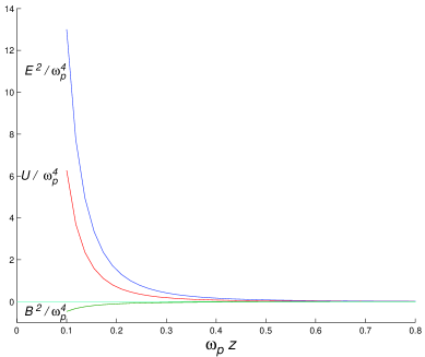
Figure 1:

The expectations of the squares of electric field, magnetic field, and energy density near the dielectric half-space are illustrated.

The plot for $\left\langle E^{2}\right\rangle$ and $\left\langle B^{2}\right\rangle,$ as well as $U$ is shown in Figure 1. As we can see from the figure, the energy density is positive. Now we consider some limiting cases.

3.4 The Fields near the Interface

To see how $U$ behaves for small $z$ (large $u$), we first perform the $t$ integration in (35), which can be done analytically, and then Taylor expand the resulting expression in the brackets in powers of $u^{-1}$. That is, we are expanding all of the integrand except for the exponential factor. To the leading order we find:

$$U\sim\frac{\sqrt{2}\omega_{p}}{64\pi}\frac{1}{z^{3}}.$$ (37)

The asymptotic behavior of the mean squared fields (36a), (36b) in this limit is

$$\left\langle E^{2}\right\rangle \sim \frac{\sqrt{2}\omega_{p}}{32\pi}\frac{1}{z^{3}},$$ (38a)

$$\left\langle B^{2}\right\rangle \sim -\frac{5\omega_{p}^{2}}{96\pi}\frac{1}{z^{2}}.$$ (38b)

We see that $\left\langle E^{2}\right\rangle$ dominates over $\left\langle B^{2}\right\rangle$, so that $U\approx 1/2\left\langle E^{2}\right\rangle;$ this is due fact that the leading order in the expression in braces in (36a) is $\propto u^{-1}$ as compared to $u^{-2}$ in (36b). If we compare these expressions to ones that would result if dispersion were not included in the calculation, it can be seen from (3.3) that in this case $\left\langle E^{2}\right\rangle\propto z^{-4}$, and same for $\left\langle B^{2}\right\rangle$ (see also [10]). As seen from (3.4), the inclusion of dispersion in the calculation reduces the power in $z$ up to two orders, but it does not remove the singularity of the results at $z=0$, as might be naively expected.

After more careful consideration, it is not surprising that dispersion alone is insufficient to render the results finite at the interface. The integrals for $\left\langle E^{2}\right\rangle$ and $\left\langle B^{2}\right\rangle$ at $z=0$ diverge quartically in a frequency cutoff. However, in general dielectric functions go as

$$\epsilon(\omega)\sim 1+O(\omega^{-2})$$ (38c)

as $\omega\rightarrow\infty$. Thus the reflection coefficients will go to zero no faster than $\omega^{-2}$, leaving the integrals quadratically divergent. This argument explains why $\left\langle B^{2}\right\rangle\propto z^{-2}$ for small $z$, but understanding the behavior of $\left\langle E^{2}\right\rangle$ requires examining the dependence of the reflection coefficients $r$ and $r^{\prime}$ upon the transverse momentum $k$. In fact the contribution of the coefficient $r$, which describes modes with the polarization vector perpendicular to the plane of incidence, does go as $z^{-2}$. This coefficient depends only upon frequency, and falls as $\omega^{-2}$ for large $\omega$, as can be seen from (34a). The coefficient $r^{\prime}$ describes modes with the polarization vector parallel to the plane of incidence, and goes to one as $\theta\rightarrow\pi/2$ (corresponding to grazing incidence) for all frequencies. It is this behavior which leads to the $z^{-3}$ singularity in $\left\langle E^{2}\right\rangle$ and hence in $U$. (The role of cutoffs for the quantized electromagnetic field in dielectrics has been discussed in more detail by Candelas [20]. Barton [21] has recently emphasized the fact that dispersion alone will not remove all divergences.)

The divergence of $U$ is not considered to be physical, but as resulting from the idealization of the wall as a perfectly smooth surface. One way of removing this singularity is to allow the position of the boundary to fluctuate [22]. It seems plausible that such effects as surface roughness, or the atomic nature of matter on small scales can also introduce a physical cutoff that makes the mean squared fields and the energy density finite everywhere.

3.5 Case of a Perfect Conductor

Now we consider the limit $\epsilon\rightarrow\infty$. In this limit, as seen from (11), (16a) and (16b), $r\rightarrow-1$, and $r^{\prime}\rightarrow 1$ . Equation (31) implies that $U$ becomes zero, as expected, and (36a) and (36b) give:

$$\left\langle E^{2}\right\rangle \sim \frac{3}{16\pi^{2}}\frac{1}{z^{4}},$$ (39)

$$\left\langle B^{2}\right\rangle \sim -\frac{3}{16\pi^{2}}\frac{1}{z^{4}}.$$ (40)

These well-known results are consistent with the asymptotic Casimir-Polder potential [23]:

$$V_{CP}\sim-\frac{3}{32\pi^{2}}\frac{\alpha_{0}}{z^{4}}=-\frac{1}{2}\alpha_{0}\left\langle E^{2}\right\rangle,$$ (41)

where $\alpha_{0}$ is the static polarizability of an atom near the interface.

4 The energy density between dielectrics

In this section we calculate the energy density in a vacuum region of width $a$ between two dielectric half-spaces. We define the dielectric constant as:

$$0<z<a:\,\,\epsilon = 1,$$

$$z<0\,\ \mathrm{and\,}\,z>a:\,\,\epsilon = \epsilon_{d}.$$ (42)

In the vacuum region, $g^{E}$ occurring in (12a) has the form

$$g^{E} =-\frac{1}{2\kappa_{0}}\left\{\frac{\exp(-\kappa_{0}\mid z-z^{\prime}\mid)+r^{2}\exp(-2\kappa_{0}a)\exp(\kappa_{0}\mid z-z^{\prime}\mid)}{r^{2}\exp(-2\kappa_{0}a)-1}+\right.$$

$$\left.+\frac{r\left[\exp(-\kappa_{0}(z+z^{\prime}))+\exp(-2\kappa_{0}a)\exp(\kappa(z+z^{\prime}))\right]}{r^{2}\exp(-2\kappa_{0}a)-1}\right\},$$ (43)

and $g^{B}$ has the same form as $g^{E,}$ with $r$ and $r^{\prime}$ interchanged, where $r$ and $r^{\prime}$ are defined in (16a) and (16b). We can now calculate the electric and magnetic fields in this region.

4.1 The Electric Field

The first and the second term on the right hand side of (21) for the present case, in the limit $z\rightarrow z^{\prime}$, are

$$\omega^{2}g^{E} = \frac{\omega^{2}}{2\kappa}\frac{1+r^{2}e^{-2\kappa a}}{1-r^{2}e^{-2\kappa a}}+\frac{\omega^{2}}{2\kappa}\frac{r(e^{-2\kappa z}+e^{-2\kappa a}e^{2\kappa z})}{1-r^{2}e^{-2\kappa a}}$$ (44)

$$(k^{2}+\nabla_{z}\nabla_{z^{\prime}})g^{B} = \frac{\omega^{2}}{2\kappa}\frac{1+r^{\prime}{}^{2}e^{-2\kappa a}}{1-r^{\prime}{}^{2}e^{-2\kappa a}}+\frac{k^{2}+\kappa^{2}}{2\kappa}\frac{r^{\prime}(e^{-2\kappa z}+e^{-2\kappa a}e^{2\kappa z})}{1-r^{\prime}{}^{2}e^{-2\kappa a}},$$ (45)

so that $\Gamma_{kk}$ becomes

$$\Gamma_{kk} =\frac{\omega^{2}}{\kappa}+\frac{\omega^{2}}{\kappa}\left(\frac{r^{2}}{e^{2\kappa a}-r^{2}}+\frac{r^{\prime}{}^{2}}{e^{2\kappa a}-r^{\prime}{}^{2}}\right)+$$

$$+\frac{1}{\kappa}\left[\omega^{2}\frac{r}{1-r^{2}e^{-2\kappa a}}+(2k^{2}-\omega^{2})\frac{r^{\prime}}{1-r^{\prime}{}^{2}e^{-2\kappa a}}\right]e^{-\kappa a}\cosh\left[\kappa(2z-a)\right].$$ (46)

We again drop the first term on the right hand side of the above expression. After introducing polar coordinates and using (11) and (46), (18) we find

$$\left\langle E^{2}\right\rangle =\frac{1}{2\pi^{2}}\int_{0}^{\infty}du\,u^{3}\int_{0}^{\frac{\pi}{2}}d\theta\,\sin(\theta)\left\{\cos^{2}(\theta)\left(\frac{r^{2}}{r^{2}-e^{2ua}}+\frac{r^{\prime}{}^{2}}{r^{\prime}{}^{2}-e^{2ua}}\right)+\right.$$

$$\left.+\left[-\cos^{2}(\theta)\frac{r}{1-r^{2}e^{-2ua}}+\left(1+\sin^{2}(\theta)\right)\frac{r^{\prime}}{1-r^{\prime}{}^{2}e^{-2ua}}\right]e^{-ua}\cosh\left[u\left(2z-a\right)\right]\right\}\,,$$ (47)

or with ($\cos(\theta)\rightarrow t$)

$$\left\langle E^{2}\right\rangle =\frac{1}{2\pi^{2}}\int_{0}^{\infty}du\,u^{3}\int_{0}^{1}dt\left\{t^{2}\left(\frac{r^{2}}{r^{2}-e^{2ua}}+\frac{r^{\prime}{}^{2}}{r^{\prime}{}^{2}-e^{2ua}}\right)+\right.$$

$$\left.+\left[-t^{2}\frac{r}{1-r^{2}e^{-2ua}}+\left(2-t^{2}\right)\frac{r^{\prime}}{1-r^{\prime}{}^{2}e^{-2ua}}\right]e^{-ua}\cosh\left[u\left(2z-a\right)\right]\right\}.$$ (48)

4.2 The Magnetic Field

In the same way, (28) leads to

$$\left\langle B^{2}\right\rangle =\frac{1}{2\pi^{2}}\int_{0}^{\infty}du\,u^{3}\int_{0}^{1}dt\left\{t^{2}\left(\frac{r^{2}}{r^{2}-e^{2ua}}+\frac{r^{\prime}{}^{2}}{r^{\prime}{}^{2}-e^{2ua}}\right)+\right.$$

$$\left.+\left[\left(2-t^{2}\right)\frac{r}{1-r^{2}e^{-2ua}}-t^{2}\frac{r^{\prime}}{1-r^{\prime}{}^{2}e^{-2ua}}\right]e^{-ua}\cosh\left[u\left(2z-a\right)\right]\right\}.$$ (49)

This expression differs from the one for $\left\langle E^{2}\right\rangle$ only in the $z$- dependent term with $r\leftrightarrow r^{\prime}$. A plot of $\left\langle E^{2}\right\rangle$ , $\left\langle B^{2}\right\rangle$ and $U$ is shown in Figure 2 for $\omega_{p}a=200.$ It can be seen in this figure that significant, but not complete cancellation occurs between $\left\langle E^{2}\right\rangle$ and $\left\langle B^{2}\right\rangle.$

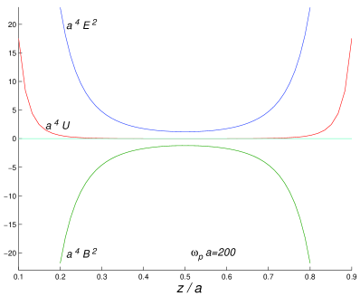
Figure 2:

The expectation values of the squared electric and magnetic fields, as well as the energy density in the vacuum region, are illustrated for $\omega_{p}a=200.$

4.3 The Energy Density

Now using (30), (48), and (49), the energy density in the vacuum region can be calculated as

$$U =\frac{1}{2\pi^{2}}\int_{0}^{\infty}du\,u^{3}\int_{0}^{1}dt\left\{t^{2}\left(\frac{r^{2}}{r^{2}-e^{2ua}}+\frac{r^{\prime}{}^{2}}{r^{\prime}{}^{2}-e^{2ua}}\right)+\right.$$

$$\left.+\left(1-t^{2}\right)\left[\frac{r}{1-r^{2}e^{-2ua}}+\frac{r^{\prime}}{1-r^{\prime}{}^{2}e^{-2ua}}\right]e^{-ua}\cosh\left[u\left(2z-a\right)\right]\right\}$$ (50)

By analyzing this expression we can make some conclusions about the sign of $U$. First we note that it is position dependent, and we also note that the first term is always negative and the second term is always positive. The overall sign of $U$ depends on the choice of $a$ and $\omega_{p}$. As $\omega_{p}a$ grows, $U$ at the midpoint decreases, becoming negative for $\omega_{p}a\approx 100$, as seen in Figure 3 and Figure 4.

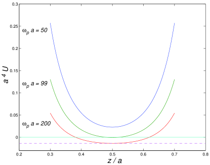
Figure 3:

The energy density in the vacuum region between two dielectric half-spaces is illustrated for three values of the parameter $\omega_{p}a.$ The dashed horizontal line is the energy density for the perfectly conducting limit, (52).

In Figure 4 we see how the energy density at the center of the vacuum region changes as the product $\omega_{p}a$ increases. It can be seen both in Figure 3 and Figure 4 that U approaches the value given in (52) as $\omega_{p}a$ becomes large. The separation at which $U$ becomes negative at the center is

$$a>a_{c}=\frac{99}{\omega_{p}}=1.3\mu{\mathrm{m}}\left(\frac{14.8e{\mathrm{V}}}{\omega_{p}}\right)\,,$$ (51)

where $14.8e{\mathrm{V}}$ is the plasma frequency of aluminum.

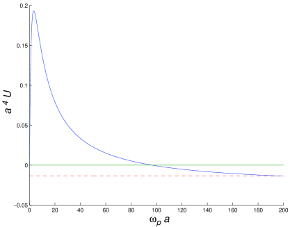
Figure 4:

The graph represents the energy density at the center of the gap between the two dielectric half-spaces as a function of $\omega_{p}a$. As seen from the graph, the energy density at center becomes negative when $\omega_{p}a\approx 99$ or larger. Again the dashed line is the perfectly conducting limit.

4.4 A Perfect Conductor Case

In the limit $\omega_{p}\rightarrow\infty$, $r\rightarrow-1$ and $r^{\prime}\rightarrow 1.$ Then only the first ($z$-independent) term survives in (50), and we get the familiar result [8]:

$$U=-\frac{\pi^{2}}{720a^{4}}.$$ (52)

It is also interesting to examine the expressions for $\left\langle E^{2}\right\rangle$ and $\left\langle B^{2}\right\rangle$ in this limit. After performing the $t$ integration, (48) can be written as

$$\left\langle E^{2}\right\rangle=\frac{1}{2\pi^{2}}\int_{0}^{\infty}du\,u^{3}\left[\frac{2}{3}\frac{1}{1-e^{2ua}}+\left(\frac{e^{-2u(a-z)}}{1-e^{-2ua}}+\frac{e^{-2uz}}{1-e^{-2ua}}\right)\right]\,,$$ (53)

and after performing the $u$ integration as

$$\left\langle E^{2}\right\rangle=-\frac{\pi^{2}}{720a^{4}}+\frac{1}{32\pi^{2}a^{4}}\left[\psi^{(3)}\left(\frac{z}{a}\right)+\psi^{(3)}\left(1-\frac{z}{a}\right)\right]\,.$$ (54)

Here $\psi^{(3)}=\frac{d^{4}}{dz^{4}}\ln\Gamma(z)$ is the polygamma function of order three. It satisfies the reflection formula [24]

$$\psi^{(3)}\left(\frac{z}{a}\right)+\psi^{(3)}\left(1-\frac{z}{a}\right)=-\pi\frac{d^{3}}{d(\frac{z}{a})^{3}}\cot\left(\pi\frac{z}{a}\right).$$ (55)

This yields

$$\left\langle E^{2}\right\rangle=-\frac{\pi^{2}}{720a^{4}}+\frac{\pi^{2}}{16a^{4}}\frac{1+2\cos^{2}(\pi\frac{z}{a})}{\sin^{4}(\pi\frac{z}{a})}.$$ (56)

In the same way, one finds

$$\left\langle B^{2}\right\rangle=-\frac{\pi^{2}}{720a^{4}}-\frac{\pi^{2}}{16a^{4}}\frac{1+2\cos^{2}(\pi\frac{z}{a})}{\sin^{4}(\pi\frac{z}{a})}.$$ (57)

These results are in agreement with those given by previous authors [25, 26].

4.5 Energy density near the Boundary

To see how $U$ grows near the interface we note that for small $z$ (large $u$), (50) becomes

$$U\approx\frac{1}{4\pi^{2}}\int_{0}^{\infty}du\,u^{3}\int_{0}^{1}dt\;\left(1-t^{2}\right)\left(r+r^{\prime}\right)e^{-2uz},$$ (58)

so it reduces to (35), the solution for one interface case. In the $z\rightarrow 0$ limit, this expression reduces to (37). By the same reasoning, the expressions for $\left\langle E^{2}\right\rangle$ and $\left\langle B^{2}\right\rangle$, (48) and (49) reduce to (36a) and (36b), respectively, in the small $z$ limit.

5 Conclusion

In this paper we have examined the mean squared fields and the energy density in the region between a pair of half-spaces filled with dispersive media. We found that these quantities diverge at the boundaries of the media, despite the inclusion of dispersion in the calculation. This divergence indicates a breakdown of a continuum description in which the dielectric function changes discontinuously at the boundary. It also shows that there is a positive self-energy density in the region outside of a single plate. Nonetheless, we have also found that it is possible for the net energy density in the region between the plates to be negative, depending upon the plate separation and the plasma frequency of the material involved. The existence of an attractive Casimir force is not an indicator of whether the energy density at the center of the plates is actually negative or not.

We have found that the energy density at the center becomes negative when $\omega_{p}a>100$. Thus for fixed plasma frequency $\omega_{p}$, the energy density always becomes negative for sufficiently large separation $a$. Of course, in this limit the magnitude of the energy density is also becoming small. Similarly, for fixed $a$, the energy density becomes negative for sufficiently large $\omega_{p}$. In the limit that $\omega_{p}\rightarrow\infty$ our results approach the constant negative energy density of the perfectly conducting plates. It should not come as a surprise that there is a regime of negative energy density. The calculation assuming perfect conductivity does have a region of validity so long as $\omega_{p}$ is large and one is not too close to one plate. Qualitatively similar behavior has recently been found for the vacuum energy density near a domain wall [27].

In this paper, we assumed a particular form for the dielectric function, (33), given by the collisionless Drude model. This is a good model for many metals especially alkali metals, and is the generic form for the dielectric function of all materials at high frequencies. Thus taking a different form for $\epsilon_{d}$ would change the details of our results, especially far from an interface, but should lead to the same limiting forms near an interface. We have also assumed zero temperature throughout this paper. For systems at room temperature, this should be a good approximation when the separations are of the order of a few micrometers. More generally, one can ignore thermal effects at distances small compared to $1/(kT)$.

Contrary to the view expressed by Lamoreaux [11], the appearance of negative energy density in a quantum field theory is very natural. One can easily find quantum states of the free quantized electromagnetic field in empty space which have local negative energy densities. A squeezed vacuum state is an example [28, 29]. The energy density of a quantized field has to be defined as a difference between that in empty Minkowski spacetime, and that in a given state and is no longer positive definite, as it was for a classical field. Apart from coupling to gravity, which produces extremely small effects, no clear way has been found to directly observe the local energy density. In certain limits, the negative energy density in a squeezed vacuum state has been shown theoretically [29] to produce an effect on the magnetic moment of a spin system. Whether this effect could ever be observed, and whether negative Casimir energy density can produce similar effects is unknown.

Acknowledgement: We would like to thank J.-T. Hsiang for valuable discussions. This work was supported in part by the National Science Foundation under Grant PHY-9800965.

References

• [1] H. B. G. Casimir, Proc. Kon. Ned. Akad. Wet. 51, 793 (1948).
• [2] M.Y. Sparnaay, Physica 24, 751 (1958).
• [3] S.K. Lamoreaux, Phys. Rev. Lett. 78, 5 (1997); erratum in Phys. Rev. Lett. 81, 5475 (1998).
• [4] U. Mohideen and A. Roy, Phys. Rev. Lett. 81, 4549 (1998).
• [5] A. Roy, C.Y. Lin and U. Mohideen, Phys. Rev. D 60, 111101 (1999).
• [6] H.B. Chan, V. A. Aksyuk, R. N. Kleiman, D. J. Bishop and Federico Capasso et al., Science 291, 1941 (2001).
• [7] G. Bressi, G. Carugno, R. Onofrio and G. Russo, Phys. Rev. Lett. 88, 041804-1 (2002).
• [8] L. S. Brown, G. J. Maclay, Phys. Rev. 184, 1272 (1969).
• [9] L.H. Ford and T.A. Roman, Phys. Rev. D 64, 024023 (2001).
• [10] A. D. Helfer and A. S. Lang, J. Phys. A: Math. Gen. 32, 1937 (1999).
• [11] S. K. Lamoreaux, Am. J. Phys. 67, 850 (1999).
• [12] E.M. Lifshitz, Zh. Eksp. Teor. Fiz. 29, 94 (1954) [Sov. Phys. JETP 2, 73 (1956)].
• [13] J. Schwinger, L. L. DeRaad, and K. A. Milton, Ann. Phys. (N.Y.) 115, 1 (1978).
• [14] J. Schwinger, Particles, Sources, and Fields Vols. I, II, (Addison-Wesley, Reading, Mass. 1970, 1973).
• [15] P.W. Milonni and M.-L. Shih, Phys. Rev. A 45, 4241 (1992).
• [16] B. Huttner and S.M. Barnett, Phys. Rev. A 46, 4306 (1992).
• [17] T. Gruner and D.-G. Welsch, Phys. Rev. A 51, 3246 (1995); 53, 1818 (1996).
• [18] R. Matloob, Phys. Rev. A 60, 50 (1999).
• [19] J. Schwinger, L.L. DeRaad, K.A. Milton, and W. Tsai, Classical Electrodynamics, (Perseus Books, 1998), p 145.
• [20] P. Candelas, Ann. Phys. (NY) 143, 241 (1982).
• [21] G. Barton, Int. J. Mod. Phys. A 17, 767 (2002).
• [22] L.H. Ford and N.F. Svaiter, Phys. Rev. D 58, 065007 (1998) .
• [23] H. B. G. Casimir and D. Polder, Phys. Rev. 73, 360 (1948).
• [24] M. Abramowitz and I.A. Stegun, eds. Handbook of Mathematical Functions, (Dover, N.Y., 1965) p260.
• [25] C. A. Lütken and F. Ravndal, Phys. Rev. A 31, 2082 (1985).
• [26] G. Barton, Phys. Lett. B 237, 559 (1990).
• [27] K.D. Olum and N. Graham, gr-qc/0205134.
• [28] C. M. Caves, Phys. Rev. D 23, 1693 (1981).
• [29] L.H. Ford, P.G. Grove, and A.C. Ottewill, Phys. Rev. D 46, 4566 (1992).