Direct measurement of optical quasidistribution functions: multimode theory and homodyne tests of Bell’s inequalities

Abstract

We develop a multimode theory of direct homodyne measurements of quantum optical quasidistribution functions. We demonstrate that unbalanced homodyning with appropriately shaped auxiliary coherent fields allows one to sample point-by-point different phase space representations of the electromagnetic field. Our analysis includes practical factors that are likely to affect the outcome of a realistic experiment, such as non-unit detection efficiency, imperfect mode matching, and dark counts. We apply the developed theory to discuss feasibility of observing a loophole-free violation of Bell’s inequalities by measuring joint two-mode quasidistribution functions by photon counting under locality conditions. We determine the range of parameters of the experimental setup that enable violation of Bell’s inequalities for two states exhibiting entanglement in the Fock basis: a one-photon Fock state divided by a 50:50 beam splitter, and a two-mode squeezed vacuum state produced in the process of non-degenerate parametric down-conversion.

I Introduction

Over the years, the field of quantum optics has gained a justified reputation of a practical testing ground for the foundations of quantum physics. The broad class of nonclassical states of optical radiation that can be feasibly generated in a laboratory has allowed one to demonstrate a variety of quantum phenomena. Furthermore, progress in the detection techniques has opened up possibilities to realize a wide range of quantum measurements on the electromagnetic fields. These advances have led in particular to two interesting developments. On one hand, it has become feasible to characterize completely the quantum state of optical radiation using the methods of so-called quantum tomography TomoReview . On the other hand, the development of sources of correlated photons based on parametric down-conversion has resulted in enormous progress in tests of Bell’s inequalities BellandDownConversion and more generally provided practical means to realize experimentally a number of theoretical proposals in the field of quantum information processing DikPDC ; KwiatPDC ; FuruSoreSCI98 .

Among different representations that can be used to characterize the quantum state of optical radiation, phase space quasidistribution functions possess several interesting features QOinPhaseSpace . They are a convenient tool in the analysis of quantum interference, as well as provide insight into the classical limit of quantum theory, including the phenomenon of decoherence ZureNAT01 . Quasidistribution functions have played an important role in the field of quantum state measurement since the first experiments on the reconstruction of the Wigner function by means of optical homodyne tomography SmitBeckPRL93 and also the earlier work on the determination of the $Q$ function using double homodyne detection WalkJMO87 . It was subsequently realized that standard experimental techniques such as homodyning and photon counting can be combined into an alternative, more direct method for measuring quasidistribution functions WallVogePRA96 ; BanaWodkPRL96 . This method directly provides the value of a quasidistribution function at a specific point of the phase space. The coordinates of that point are defined by the amplitude and the phase of an auxiliary coherent field used for homodyning. The basic idea of the direct method is to perform photocounting on the signal field superposed at a highly transmissive beam splitter with a relatively strong coherent field. With a good approximation, such a procedure adds a coherent amplitude to the signal field, while retaining all the quantum fluctuations it initially contained. The unbalanced homodyning scheme for measuring the Wigner function has been realized in a proof-of-principle experiment in Ref. BanaRadzPRA99 .

The development of unbalanced homodyning has led to a novel proposal for testing Bell’s inequalities in optical systems BanaWodkPRL99 . The proposal was based on an observation that the two-mode generalization of the direct scheme for measuring quasidistribution functions could be straightforwardly reinterpreted as a standard arrangement for measuring correlation functions between two spatially separated apparatuses satisfying the locality conditions. The role of dichotomic variables in this proposal is played either by the parity of the registered number of photons, or by the presence of any number of photons. It was demonstrated theoretically for a selection of input states that such correlation functions are capable of violating Bell’s inequalities BanaWodkPRL99 ; BanaWodkPRA98 . In addition, the character of measured observables does not require supplementary assumptions that were necessary in the previous proposals for testing Bell’s inequalities using balanced homodyning GranPotaYurkPRA88 . This has opened up yet another route to optical tests of Bell’s inequalities, alternative to those based on polarization BellandDownConversion or frequency-time entanglement FrequencyBell . Recently, the possibility of testing Bell’s inequalities based on homodyning and photon counting has been explored experimentally by Kuzmich et al. KuzmWalmPRL00 .

The purpose of the present paper is two-fold. In the first part, we provide a complete multimode theory of the direct method for measuring quasidistribution functions. Previous theoretical discussions of unbalanced homodyning were based on an assumption that the beams interfered at a beam splitter contained single excited modes with perfectly matching spatio-temporal characteristics. Here we will analyze the case when both the beams are described by general electromagnetic field operators. We will demonstrate that if the signal field comprizes several excited modes, the full multimode quasidistribution function of the signal field can be measured directly by an appropriate spatio-temporal shaping of the auxiliary coherent field used for homodyning. Interestingly, this measurement scheme does not depend on whether the excited modes can be separated before the detection or not. The only observable that needs to be determined is the statistics of the total number of photons in all the modes of interest. The general multimode treatment will also allow us to address rigorously the problem of imperfect mode matching between the signal and probe fields. We will show that the effect of mode mismatch is essentially different from that occurring in balanced homodyne detection BHDMismatch , where it simply contributes to the overall detection efficiency. For completeness, we will also discuss here other practical aspects that are likely to affect a realistic experiment, such as dark counts.

In the second part of this paper, we apply the multimode theory to perform a feasibility study of tests of Bell’s inequalities based on unbalanced homodyning. We focus our attention on two quantum states of optical radiation: a single photon divided by a 50:50 beam splitter and a two-mode squeezed vacuum state. Both these states can be practically generated using spontaneous parametric down-conversion in media with $\chi^{(2)}$ nonlinearity. We determine here the range of experimental parameters such as detector efficiency and mode matching, which enable violation of Bell’s inequalities. Generation of a one photon Fock state in a controlled spatio-temporal mode has been recently demonstrated by Lvovsky et al. LvovHansPRL01 , who were able to achieve a sufficient overlap with the local oscillator field to demonstrate the negativity of the corresponding Wigner function. This significant experimental result encourages us to examine more closely the possibility of testing Bell’s inequality by homodyning a single photon divided on a beam splitter. Generation of the second state studied here, i.e. the two mode squeezed vacuum state, also attracts presently a great deal of interest as one of the constructional primitives in quantum information processing based on continuous variables FuruSoreSCI98 ; ContinuousQIP . We note that in contrast to a typical scenario considered in this context, involving measurements of continuous quadrature observables, we will be dealing with a discrete, binary detection scheme. This example suggests that continuous-variable entanglement could perhaps be useful also for implementations of other quantum information protocols relying on binary logic ChenPanPRL02 .

We would like to stress here that the operational meaning of two-mode quasidistribution functions as nonlocal correlation functions depends critically on the specific experimental scheme used for the measurement. In order to perform a valid test of quantum nonlocality, the measured quantities must satisfy the local reality conditions that are assumed in the derivation of the corresponding Bell’s inequality. In particular, if standard Bell’s inequalities derived for binary measurements on spin-1/2 particles are to be applied to a quantum optical experiment, the output signals from the photodetectors have to be converted into dichotomic variables on a shot-by-shot basis. This condition is fulfilled by the direct scheme based on unbalanced homodyning, where in each run one either registers the photon number parity, or checks for the presence of any number of photons. In contrast, this is not the case for the optical homodyne tomography scheme, where the Wigner function is reconstructed by an application of tomographic back-projection algorithms to quadrature statistics obtained from balanced homodyne detection. Obviously, such a procedure cannot be performed on the shot-by-shot basis. This difference can be best seen on the example of the two-mode squeezed vacuum state: it is well known that detection of quadratures has a straightforward local hidden variable model based on the Wigner representation, whereas it has been demonstrated that unbalanced homodyning can reveal the nonlocality of this state. The above argument invalidates the claim of Ref. WuPRA00 that in order to improve the detection efficiency, unbalanced homodyning can be simply replaced in tests of Bell’s inequalities by optical homodyne tomography SmitBeckPRL93 or cascaded homodyning KisKissPRA99 . We note that balanced homodyne detection can be used to test Bell’s inequalities in other proposals, that are for example based on a legitimate procedure of binary classification of the result of a quadrature measurement GilcDeuaPRL98 ; DragBanaPRA01 .

This paper is organized as follows. We start in Sec. II from analyzing multimode interference at an unbalanced beam splitter, and demonstrate, using an appropriate modal decomposition, how the overall statistics of photocounts can be related to multimode quasidistribution functions of the input signal field. In Sec. III we discuss effects of imperfections in a practical experimental setup, including non-unit detection efficiency, dark counts, and imperfect mode overlap. We find that these three factors have distinctively different effects on the measured observables. Next, we review in Sec. IV how the two-mode case can be used to test Bell’s inequalities, and derive realistic expressions for measured correlation functions that include effects of dominant experimental imperfections. These correlation functions are analyzed in detail in the following sections using two specific examples of two-mode input states: a one-photon Fock state divided on a 50:50 beam splitter in Sec. V, and a two-mode squeezed vacuum state in Sec. VI. In particular, we find the range of experimental parameters where a violation of Bell’s inequalities can be observed. Finally, Sec. VII concludes the paper.

II Multimode theory

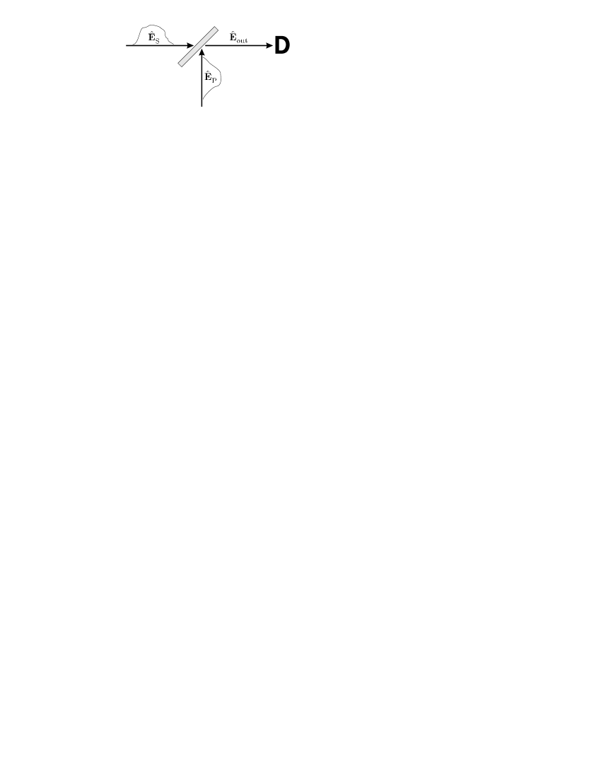
Figure 1: Experimental arrangement consisting of signal and probe fields, interfered at a beam splitter characterized by a power transmission $T$. The output port of the beam splitter is monitored by a photon counting detector integrating the incident light over its active surface.

In this section we develop the full multimode theory of the direct scheme for measuring the quantum optical quasidistribution functions proposed in Refs. WallVogePRA96 ; BanaWodkPRL96 . A general arrangement depicted in Fig. 1 consists of two fields, named as the signal and the probe, interfered at a beam splitter characterized by a power transmission $T$. The output port of the beam splitter is monitored by a photon counting detector integrating the incident light over its active surface. In the single-mode description of light incident on a beam splitter it is sufficient to use a pair of annihilation operators referring to the signal and the probe fields, respectively. The spatio-temporal characteristics of these two modes are not important in this approach as long as it is implicitly assumed that the modes are matched perfectly at the beam splitter. We shall free our further analysis from these simplifying assumptions.

II.1 Interference at a beam splitter

Let us denote by $\hat{\bf E}^{(+)}_{\text{\scriptsize out}}({\bf r},t)$ the positive-frequency part of the electric field operator at the surface of the detector. This field is a superposition of the signal and the probe fields combined at the beam splitter BS. Mathematical representation of this combination is a slightly intricate matter. If we wanted to proceed rigorously and express $\hat{\bf E}_{\text{\scriptsize out}}^{(+)}({\bf r},t)$ in terms of the signal and probe field operators before the beam splitter, we would have to introduce appropriate propagators for the fields in the presence of the beam splitter QO-VWW . Instead, we shall choose different notation for the signal and the probe fields, which will make the discussion more intuitive. Let us denote by $\hat{\bf E}_{\text{S}}^{(+)}({\bf r},t)$ the electric field operator of the signal beam that would fall onto the detector surface in the absence of the beam splitter BS. Analogously, let $\hat{\bf E}_{\text{P}}^{(+)}({\bf r},t)$ be the probe field at the detector surface, assuming that the beam splitter BS was replaced by a perfectly reflecting mirror. With these definitions, the field $\hat{\bf E}^{(+)}_{\text{\scriptsize out}}({\bf r},t)$ resulting from the interference of the signal and the probe beams is given simply by

$$\hat{\bf E}^{(+)}_{\text{\scriptsize out}}({\bf r},t)=\sqrt{T}\hat{\bf E}^{(+)}_{\text{S}}({\bf r},t)-\sqrt{1-T}\hat{\bf E}^{(+)}_{\text{P}}({\bf r},t),$$ (1)

where $T$ denotes the beam splitter power transmission coefficient. We have assumed here that the characteristics of the beam splitter are constant over the spectral and polarization range of the considered fields. Further, we shall assume that the detected fields are quasi-monochromatic with the central frequency $\omega_{0}$. This will allow us to relate easily the number of photons to the energy of the field absorbed by the detector. Assuming that the direction of propagation of the field $\hat{\bf E}^{(+)}_{\text{\scriptsize out}}({\bf r},t)$ is perpendicular to the detector, the operator of the photon flux through the detector surface reads:

$$\hat{\cal J}_{\text{\scriptsize out}}=\frac{2\epsilon_{0}c}{\hbar\omega_{0}}\int_{\Delta t}\text{d}t\int_{D}\text{d}^{2}{\bf r}\,\hat{\bf E}^{(-)}_{\text{\scriptsize out}}({\bf r},t)\hat{\bf E}^{(+)}_{\text{\scriptsize out}}({\bf r},t),$$ (2)

where $\hat{\bf E}^{(-)}_{\text{out}}({\bf r},t)=[\hat{\bf E}^{(+)}_{\text{out}}({\bf r},t)]^{\dagger}$, and the temporal and the spatial integrals are performed respectively over the detector opening time $\Delta t$ and its active surface $D$. The probability $p_{n}$ of registering $n$ counts on a photodetector is given by

$$p_{n}=\left\langle:e^{-\eta\hat{\cal J}_{\text{out}}}\frac{(\eta\hat{\cal J}_{\text{\scriptsize out}})^{n}}{n!}:\right\rangle_{\text{S,P}},$$ (3)

where $\eta$ is the detector quantum efficiency and $:\ldots:$ denotes normal ordering. Following the idea of Ref. BanaWodkPRL96 , we shall use the measured photocount statistics to evaluate the expression of the form

$$\Pi(s)=\sum_{n=0}^{\infty}\left(\frac{s+1}{s-1}\right)^{n}p_{n},$$ (4)

where $s$ is a real parameter, assumed to be nonpositive in order to assure convergence of the series on the right-hand side of the above formula. We will see that in the limit of negligible losses, the parameter $s$ describes the ordering of the measured quasidistribution function. The quantity in Eq. (4) can be written in terms of the photon flux operator as:

$$\Pi(s)=\left\langle:\!\exp\left(-\frac{2\eta\hat{\cal J}_{\text{\scriptsize out}}}{1-s}\right)\!:\right\rangle_{\text{S,P}}.$$ (5)

If a coherent field is used as the probe, we may immediately evaluate the quantum expectation value over the probe field and obtain:

$$\Pi(s) = \left\langle:\exp\left(-\frac{4\eta\epsilon_{0}c}{\hbar\omega_{0}(1-s)}\int_{\Delta t}\text{d}t\int_{D}\text{d}^{2}{\bf r}\,\left[\sqrt{T}\hat{\bf E}_{\text{S}}^{(-)}({\bf r},t)-\sqrt{1-T}{\bf E}_{\text{P}}^{\ast}({\bf r},t)\right]\right.\right.$$ (6)

$$\times\left.\left.\vphantom{\frac{4\eta\epsilon_{0}c}{\hbar\omega_{0}(1-s)}\int_{\Delta t}\text{d}t\int_{D}\text{d}^{2}{\bf r}}\left[\sqrt{T}\hat{\bf E}^{(+)}_{\text{S}}({\bf r},t)-\sqrt{1-T}{\bf E}_{\text{P}}({\bf r},t)\right]\right):\right\rangle,$$

where ${\bf E}_{\text{P}}({\bf r},t)=\langle\hat{\bf E}^{(+)}_{\text{P}}({\bf r},t)\rangle_{\text{P}}$ is the amplitude of the electric field of the probe beam. Thus, we can simply replace the coherent probe field operators with their expectation values in all normally ordered expressions involving the photocount statistics.

II.2 Modal decomposition

We will now consider the signal field $\hat{\bf E}^{(+)}_{\text{S}}({\bf r},t)$ in which a finite number of $M$ modes is possibly excited. We shall denote the corresponding annihilation operators by $\hat{a}_{i}$, and the mode functions by ${\bf u}_{i}({\bf r},t)$, where $i=1,2,\ldots M$. Our goal will be to relate the photon statistics $p_{n}$ to the multimode quasidistribution characterizing these modes. Thus we decompose the signal field $\hat{\bf E}^{(+)}_{\text{S}}({\bf r},t)$ in the form

$$\hat{\bf E}^{(+)}_{\text{ S}}({\bf r},t)=\sum_{i=1}^{M}\hat{a}_{i}{\bf u}_{i}({\bf r},t)+\hat{\bf V}({\bf r},t),$$ (7)

where the operator $\hat{\bf V}({\bf r},t)$ is a sum of all the other modes remaining in the vacuum state. This part of the field does not contribute to the detector counts in the normally ordered expression given in Eq. (6).

Further, we shall assume that virtually all the excited part of the signal field is absorbed by the detector within the gate opening time. This allows us to write orthonormality relations for the mode functions ${\bf u}_{i}({\bf r},t)$ in the form

$$\frac{2\epsilon_{0}c}{\hbar\omega_{0}}\int_{\Delta t}\text{d}t\int_{D}\text{d}^{2}{\bf r}\,{\bf u}_{i}^{\ast}({\bf r},t){\bf u}_{j}({\bf r},t)=\delta_{ij},$$ (8)

where the integrals are restricted to the domain defined by the detection process. With these assumptions, we may simplify the exponent of Eq. (6). It is convenient to introduce dimensionless amplitudes $\alpha_{i}$, which are projections of the probe field onto the signal mode functions:

$$\alpha_{i}=\frac{2\epsilon_{0}c}{\hbar\omega_{0}}\int_{\Delta t}\text{d}t\int_{D}\text{d}^{2}{\bf r}\,{\bf u}_{i}^{\ast}({\bf r},t){\bf E}_{\text{P}}({\bf r},t).$$ (9)

These amplitudes describe the parts of the coherent probe field ${\bf E}_{\text{P}}({\bf r},t)$ that match the corresponding modes in the signal field. Furthermore, let us also denote by ${\cal J}_{\text{P}}$ the average total number of photons in the probe field:

$${\cal J}_{\text{P}}=\frac{2\epsilon_{0}c}{\hbar\omega_{0}}\int_{\Delta t}\text{d}t\int_{D}\text{d}^{2}{\bf r}\,|{\bf E}_{\text{P}}({\bf r},t)|^{2}.$$ (10)

Using this notation, we may write the quantity $\Pi(s)$ determined from the photocount statistics as:

$$\Pi(s) = \left\langle:\exp\left[-\frac{2\eta T}{1-s}\sum_{i=1}^{M}\left(\hat{a}_{i}^{\dagger}-\sqrt{\frac{1-T}{T}}\alpha_{i}^{\ast}\right)\left(\hat{a}_{i}-\sqrt{\frac{1-T}{T}}\alpha_{i}\right)\right]:\right\rangle$$ (11)

$$\times\exp\left[-\frac{2\eta(1-T)}{1-s}\left({\cal J}_{\text{P}}-\sum_{i=1}^{M}|\alpha_{i}|^{2}\right)\right].$$

The expectation value appearing in the above expression can be identified, up to a normalization factor, as an $M$-mode quasidistribution function. This equivalence becomes clear if we recall the normally ordered definition of the generalized $s$-ordered quasidistribution functions CahiGlauPR69 :

$$W(\gamma_{1},\ldots,\gamma_{M};s)=\left(\frac{2}{\pi(1-s)}\right)^{M}\left\langle:\!\exp\left(-\frac{2}{1-s}\sum_{i=1}^{M}(\hat{a}_{i}^{\dagger}-\gamma_{i}^{\ast})(\hat{a}_{i}-\gamma_{i})\right)\!:\right\rangle.$$ (12)

After the identification of the parameters we obtain that:

$$\Pi(s) = \left(\frac{\pi(1-s)}{2\eta T}\right)^{M}W_{\text{S}}\left(\sqrt{\frac{1-T}{T}}\alpha_{1},\ldots,\sqrt{\frac{1-T}{T}}\alpha_{M};-\frac{1-s-\eta T}{\eta T}\right)$$ (13)

$$\times\exp\left[-\frac{2\eta(1-T)}{1-s}\left({\cal J}_{\text{P}}-\sum_{i=1}^{M}|\alpha_{i}|^{2}\right)\right].$$

The exponential factor multiplying the quasidistribution function involves the difference between the average total number of photons $\hat{\cal J}_{P}$ in the probe field and the sum $\sum_{i=1}^{M}|\alpha_{i}|^{2}$ describing the number of the probe field photons that match the corresponding modes of the signal field. This factor results from the part of the probe field that is orthogonal (in the sense of spatio-temporal overlap defined by Eq. (8)) to the mode functions describing the excited component of the signal beam, and it becomes identically equal to one if the probe field exactly matches the $M$ signal modes of interest. The matching condition can be written as:

$${\bf E}_{\text{P}}({\bf r},t)=\sum_{i=1}^{M}\alpha_{i}{\bf u}_{i}({\bf r},t).$$ (14)

In such a case of perfect mode matching on the beam splitter the quantity $\Pi(s)$ calculated from the photocount statistics is equal, up to a constant multiplicative factor, to the value of a multimode quasidistribution function with the ordering $-(1-s-\eta T)/\eta T$, taken at the point $(\sqrt{(1-T)/T}\alpha_{1},\ldots,\sqrt{(1-T)/T}\alpha_{M})$. This result implies a simple recipe for measuring multimode quasidistribution functions point-by-point. What one needs to do in order to determine the value of a quasidistribution function at a specific point, is to prepare the coherent probe field in an appropriate superposition defined by Eq. (14), and to measure the photocount statistics of the probe and signal fields combined at an unbalanced beam splitter. The sum over the photocount statistics evaluated according to Eq. (4) yields directly the value of the quasidistribution function. The ordering of the measured quasidistribution depends on the overall losses of the signal field characterized by the product $\eta T$, as well as the parameter $s$ used to evaluate the sum over the count statistics. The allowed range of the parameter $s$ has been discussed previously BanaWodkJMO97 in the context of the statistical uncertainty. It has been shown that in order to keep the statistical error bounded, the parameter $s$ needs to be taken nonpositive. As in the single-mode case, the highest attainable ordering of the measured quasidistribution function is equal to $-(1-\eta T)/\eta T$, which in the limit of ideal lossless detection yields zero, thus corresponding to the detection of the Wigner function. An interesting feature of this scheme is that there is no need to resolve contributions to the photocount statistics from each of the modes separately; the only observable that needs to be reconstructed is the sum over the statistics of the total number of photocounts.

One should note that in a realistic situation it is not always possible to measure the complete photocount statistics. Most of the single-photon detectors used presently, such as avalanche photodiodes operated in the Geiger mode, yield only a binary response telling whether any number of photons has been registered or not. We can easily specialize our previous considerations to include this case by taking the limit $s\rightarrow-1$, in which the sum $\Pi(s)$ reduces to

$$\lim_{s\rightarrow-1}\Pi(s)=p_{0},$$ (15)

i.e. the probability of registering zero counts on the detectors. Thus, if only the information about the presence or absence of photons is available, we can reconstruct a quasidistribution function with the ordering $-(2-\eta T)/\eta T$, which in the limit of lossless detection reduces to $-1$ corresponding to the measurement of a $Q$ function.

More generally, one can consider application of a detection scheme that can resolve the number of photons up to a certain value, such as the visible light photon counter KimTakeAPL99 , detector cascading KokBrauPRA01 , or the loop detector BanaWalmXXX02 . In this case, one is limited to sampling these regions of the phase space where the photon statistics effectively vanishes above the cut-off value of the used detector. Several examples of photon statistics have been analyzed in detail in Ref. BanaWodkJMO97 . It has been found in certain cases that the occurence of structures in the phase space can be related to destructive interference at the unbalanced beam splitter, resulting in low photon numbers seen by the detectors. These structures could thus be measured using detectors with restricted multiphoton resolution.

II.3 Multiple detectors

The direct scheme for measuring multimode quasidistribution functions can be easily extended to the case when some of the modes are separated in space. In this case, each mode (or a group of spatially overlapping modes) needs to be displaced in the phase space by combining it at a beam splitter with a coherent probe field, and then measured using a photon counting detector. For simplicity, let us assume that we are dealing with two separate beams labelled with $A$ and $B$. Such a setting, with the detection procedures satisfying locality conditions, will serve as a scheme for testing Bell’s inequalities discussed in the subsequent sections of this paper. Generalization of our results to more that two beams will follow in a straightforward manner. The two detectors in our setup yield photocount statistics $p_{A,n}$ and $p_{B,n}$. We will show that Eq. (4) applied to the statistics of the total number of counts $p_{n}$, defined as:

$$p_{n}=\sum_{m=0}^{n}p_{A,m}p_{B,n-m}$$ (16)

yields the joint quasidistribution function of the signal field.

In order to fix the notation, let us assume that $M_{A}$ and $M_{B}$ modes are excited in the beams $A$ and $B$ respectively, and denote the corresponding annihilation operators by $\hat{a}_{i}$ and $\hat{b}_{i}$. The displacement of the signal field can be performed by preparing the probe field in the form of two beams interfering with the beams $A$ and $B$. A calculation completely analogous to the one presented in the previous section shows that $\Pi(s)$ evaluated from the overall count statistics has the following form:

$$\Pi(s) = \left\langle:\!\exp\left(-\frac{2\eta T}{1-s}\sum_{i=1}^{M_{A}}\left(\hat{a}_{i}^{\dagger}-\sqrt{(1-T)/T}\alpha_{i}^{\ast}\right)\left(\hat{a}_{i}-\sqrt{(1-T)/T}\alpha_{i}\right)\right)\right.$$ (17)

$$\left.\otimes\exp\left(-\frac{2\eta T}{1-s}\sum_{i=1}^{M_{B}}\left(\hat{b}_{i}^{\dagger}-\sqrt{(1-T)/T}\beta_{i}^{\ast}\right)\left(\hat{b}_{i}-\sqrt{(1-T)/T}\beta_{i}\right)\right)\!:\right\rangle$$

$$\times\exp\left[-\frac{2\eta(1-T)}{1-s}\left({\cal J}_{\text{P},A}-\sum_{i=1}^{M_{A}}|\alpha_{i}|^{2}+{\cal J}_{\text{P},B}-\sum_{i=1}^{M_{B}}|\beta_{i}|^{2}\right)\right]$$

Here $\alpha_{i}$ and $\beta_{i}$ are the probe field amplitudes matching the modes of the signal field. They are defined analogously to Eq. (9), with the integration over the detection time and the active area of the appropriate detector $A$ or $B$. Similarly, ${\cal J}_{\text{P},A}$ and ${\cal J}_{\text{P},B}$ are the intensities of the two probe beams expressed in the photon number units. For simplicity we have assumed here that the two detectors have the same quantum efficiency $\eta$, and also that both the beam splitters are characterized by the same transmission coefficient $T$. As before, the expectation value in Eq. (17) can be identified as proportional to a multimode quasidistribution function, and the second exponential factor results from imperfect matching of the probe field to the signal modes.

III Practicalities

In this section, we will discuss the effect of experimental imperfections that are likely to occur in a practical realization of the proposed scheme. First, we shall analyze the role of dark counts in the described measurement scheme. Secondly, we will study on a simple example the effect of imperfect matching between the signal and probe fields at the beam splitter.

III.1 Dark counts

The first effect that needs to be taken into account is the dark noise of the detectors. Apart from the photocounts originating from the measured field, the detector can generate additional counts. These can result from thermal excitations in the active material of the photodetector, or from absorption of stray light. We shall make a simplifying assumption in our analysis that the dark counts are not correlated statistically with the photocounts generated by the field of interest. Thus we neglect for example the phenomenon of afterpulsing in avalanche photodiodes, which consists in generating signal by carriers trapped after detection of preceding photons. Under this assumption the statistics of detector counts $p_{n}$ can be represented as a discrete convolution of the statistics of counts originating from the measured field $p_{{\text{F}},n}$ and the statistics of dark counts $p_{{\text{D}},n}$:

$$p_{n}=\sum_{m=0}^{n}p_{{\text{F}},m}p_{{\text{D}},n-m}.$$ (18)

It is then straightforward to check that the sum over the count statistics factorizes into the product:

$$\sum_{n=0}^{\infty}\left(\frac{s+1}{s-1}\right)^{n}p_{n} = \sum_{m=0}^{\infty}\left(\frac{s+1}{s-1}\right)^{m}p_{{\text{F}},m}$$ (19)

$$\times\sum_{n=0}^{\infty}\left(\frac{s+1}{s-1}\right)^{n}p_{{\text{D}},n}$$

This expression means that as long as the dark counts are uncorrelated with the counts generated by the photons from the measured fields, $\Pi(s)$ simply becomes rescaled by a constant factor defined only by the dark count statistics. Therefore in order to include the effect of dark counts in our analysis we only need to multiply the previous formulas by this constant factor. Furthermore, if we choose $s=-1$, this multiplicative factor simply becomes $p_{{\text{D}},0}$, i.e. the probability of a zero dark count event.

III.2 Mode mismatch

In a realistic situation, it is virtually impossible to achieve ideal matching between the signal and probe fields at a beam splitter. Consequently, experimental results will usually be affected by imperfect mode matching. In order to analyze this effect in quantitative terms and estimate its importance, we will now consider the practical measurement of a single quasidistribution function. For this purpose, we will assume that $M=1$, i.e. that only one mode is excited in the decomposition of the signal field defined in Eq. (7), and for simplicity we shall drop the index labelling its annihilation operator $\hat{a}$ and the corresponding mode function ${\bf u}({\bf r},t)$. In the further analysis, it will be convenient to introduce the mode matching parameter $\xi$ defined by:

$$\xi=\frac{|\alpha|^{2}}{{\cal J}_{\text{P}}}=\frac{2\epsilon_{0}c}{\hbar\omega_{0}}\frac{\displaystyle\left|\int_{\Delta t}\text{d}t\int_{D}\text{d}^{2}{\bf r}\,{\bf u}^{\ast}({\bf r},t){\bf E}_{\text{P}}({\bf r},t)\right|^{2}}{\displaystyle\int_{\Delta t}\text{d}t\int_{D}\text{d}^{2}{\bf r}\,|{\bf E}_{\text{P}}({\bf r},t)|^{2}}.$$ (20)

It follows directly from the Schwarz inequality that the parameter $\xi$ defined in the above way lies between $0$ and $1$. The value $\xi=1$ corresponds to the perfect overlap between the signal and the probe modes, whereas the value $\xi=0$ means that the signal and probe fields are completely orthogonal.

Using the mode matching parameter, we can write $\Pi(s)$ as:

$$\Pi(s) = \frac{\pi(1-s)}{2\eta T}W\left(\sqrt{\frac{1-T}{T}}\alpha;-\frac{1-s-\eta T}{\eta T}\right)$$ (21)

$$\times\exp\left(-\frac{2\eta(1-T)}{1-s}\frac{1-\xi}{\xi}|\alpha|^{2}\right).$$

It is seen that in the case of imperfect mode matching the measured quasidistribution function is multiplied by a Gaussian envelope centered at the origin of the phase space. The width of the Gaussian depends on the factor $(1-\xi)/\xi$, which grows with the increasing mismatch between the signal and probe fields. Thus, the effect of the mode mismatch is more severe in the outer regions of the phase space, where the amplitude of the signal quasidistribution function is suppressed by the Gaussian envelope resulting from the mode mismatch.

It is interesting to note that the effect of the mode mismatch in our scheme is quite different from that occurring in balanced homodyne detection BHDMismatch . In the latter case, the mode matching parameter simply multiplies the overall efficiency of the homodyne detector, and is equivalent to additional losses of the signal field. In contrast, Eq. (21) includes the quantum efficiency and the mode matching parameter in two nonequivalent ways, and the strength of the effect of the mode mismatch depends on the selected point of the phase space. This difference between balanced and unbalanced homodyning can be easily understood by comparing the relative intensities of the signal and local oscillator fields at the detectors. In the balanced case, only the part of the signal field matching the shape of the local oscillator affects noticeably the photocount statistics. In the case of unbalanced homodyning, both the signal and local oscillator fields have comparable intensities at the exit of the superposing beam splitter and contribute with similar strengths to the count statistics.

In a practical situation, it is convenient to relate the mode matching parameter $\xi$ to the interference visibility on the beam splitter used to combine the signal and probe fields. Suppose that we can replace the signal field of interest by a coherent state $|\alpha_{\text{S}}\rangle$ prepared in exactly the same spatio-temporal mode. A simple calculation shows that the average light intensity ${\cal J}_{\text{out}}$ received by the detector, expressed in the photon number units, is given by:

$${\cal J}_{\text{out}}=(1-\xi)T|\alpha_{\text{S}}|^{2}+|\sqrt{\xi T}\alpha_{\text{S}}-\sqrt{(1-T)\xi}\alpha|^{2}.$$ (22)

The minimum intensity of the output light that can be obtained by varying the phase and the amplitude of the probe field while keeping $\alpha_{\text{S}}$ fixed is given by:

$${\cal J}_{\text{min}}=(1-\xi)T|\alpha_{\text{S}}|^{2}$$ (23)

If we now change the phase of the probe field by $\pi$, this will maximize the output intensity for the fixed absolute value of the probe field amplitude, thus yielding:

$${\cal J}_{\text{max}}=(1+3\xi)T|\alpha_{\text{S}}|^{2}.$$ (24)

Consequently, the interference visibility $\upsilon$ defined in the standard way can be expressed in terms of the parameters used thorough our discussion as:

$$\upsilon=\frac{{\cal J}_{\text{max}}-{\cal J}_{\text{min}}}{{\cal J}_{\text{max}}+{\cal J}_{\text{min}}}=\frac{2\xi}{1+\xi}.$$ (25)

Inverting this relation we obtain that $\xi=\upsilon/(2-\upsilon)$. Thus, the measurement of the interference visibility based on the method sketched above can yield an estimate for the quality of the mode matching in the experimental setup. This approach has been used in Ref. BanaRadzPRA99 to analyze the shape of the experimentally measured Wigner function of a coherent state.

IV Testing Bell’s inequalities

We will now specialize the general theory developed in the previous sections to the case when two light modes in an entangled state are sent towards a pair of spatially separated unbalanced homodyne detectors. It has been suggested in previous theoretical works BanaWodkPRL99 ; BanaWodkPRA98 that such a setup can be used to test Bell’s inequalities. In the proposed approach, the standard spin measurements are replaced by dichotomic observables derived from the photocount statistics, and the auxiliary coherent fields provide adjustable parameters that can be selected by the observers under locality conditions. Our goal here will be to perform a complete realistic analysis of the proposed scheme, including all the practical factors that are likely to affect the outcome of the proposed experiment.

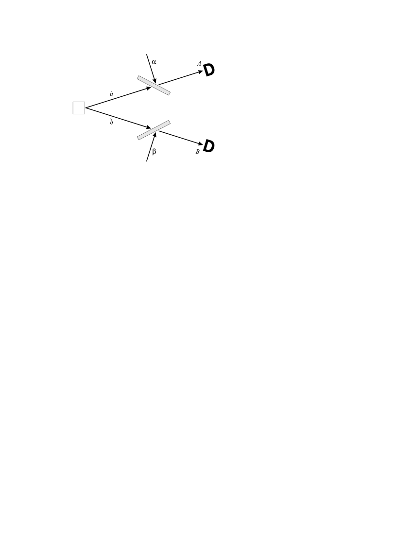
Figure 2: Two entangled and spatially separated light beams fall onto unbalanced homodyne detectors composed of photon counters preceded by high-transmission beam splitters with auxiliary coherent fields entering through the sideway input ports.

Let us first summarize briefly the unbalanced homodyne setup proposed to test Bell’s inequalities, depicted in Fig. 2. Two entangled and spatially separated light beams fall onto unbalanced homodyne detectors composed of photon counters preceded by high-transmission beam splitters with auxiliary coherent fields entering through the sideway input ports. The operation of such a setup can be easily reformulated in terms of a standard scheme for testing Bell’s inequalities with measuring apparatuses that provide dichotomic outcomes. The binary variable we will be interested in is whether any number of photons has been registered by a photon counting detector, without resolving the actual number of photons. Such a measurement corresponds formally to a standard test whether a particle has passed through a polarization analyzer. It is important to note that this dichotomic measurement can be feasibly realized with the help of avalanche photodiodes operated in the Geiger mode that are not capable of providing the number of photons triggering the avalanche signal. At the same time, we can utilize other favorable characteristics of avalanche photodiodes, such as relatively high quantum efficiency and low dark count rates. The pair of non-commuting observables at each receiving station will be established by selecting two different complex amplitudes of the coherent field added to the signal beam at the beam splitter. The choice of the coherent state amplitudes thus corresponds to two possible orientations of polarization analyzers used in standard experiments on Bell’s inequalities. In each experimental run, the observers select randomly the amplitudes of the coherent fields and record the response of their photon counting detectors. In practice, all the coherent light beams in the setup need to be derived from the same source in order to ensure fixed phase relationships. This of course fully complies with the assumptions underlying Bell’s inequalities as long as the amplitude and the phase of auxiliary coherent beams are adjusted by the two parties under locality conditions. We will now discuss in detail correlation functions constructed from these data and analyze their nonlocal character.

In order to formulate our discussion in terms of quasidistribution functions and utilize results derived in Secs. II and III, we shall attribute the value $+1$ to events a photon counting detector did not click and $0$ when any non-zero number of photons was registered. In such a case, we can specialize the results from the previous sections by taking the value of the $s$ parameter used in the definition of the sum over the photon count statistics in Eq. (4) equal to $s=-1$. Then the whole sum over the photon count statistics reduces simply to $p_{0}$, i.e. the probability of observing zero photons, which corresponds exactly to our assignment of numerical values to experimental outcomes. Our test of Bell’s inequalities is based on measuring the joint and marginal probabilities of such “photon silence” events, which we shall denote respectively by $Q(\tilde{\alpha},\tilde{\beta})$ and $Q(\tilde{\alpha})$ or $Q(\tilde{\beta})$. Here $\tilde{\alpha}$ and $\tilde{\beta}$ are complex amplitudes of the coherent fields rescaled by a certain factor whose value we will discuss later. As the probability of a no-count event is obviously bounded between $0$ and $1$, the nonlocal character of the measured correlation functions can be tested with the help of the standard Clauser-Horne inequality ClauHornPRD74 :

$$-1\leq{\cal CH}\leq 0,$$ (26)

where the combination ${\cal CH}$ is constructed with the help of the formula:

$${\cal CH} = Q(\tilde{\alpha}_{1},\tilde{\beta}_{1})+Q(\tilde{\alpha}_{1},\tilde{\beta}_{2})+Q(\tilde{\alpha}_{2},\tilde{\beta}_{1})-Q(\tilde{\alpha}_{2},\tilde{\beta}_{2})$$ (27)

$$-Q(\tilde{\alpha}_{1})-Q(\tilde{\beta}_{1}).$$

Here $\tilde{\alpha}_{1},\tilde{\alpha}_{2}$ and $\tilde{\beta}_{1},\tilde{\beta}_{2}$ denote the two settings of the coherent fields used at the respective detectors.

We will now derive expressions for the joint and marginal probabilities of “photon silence” events that include possible imperfections of the experimental setup. For simplicity, we shall assume that the excited parts of the fields travelling to the homodyne detectors can be described by single-mode annihilation operators $\hat{a}$ and $\hat{b}$. The expression for the joint zero-count event is then simply given by Eq. (17) with $s=-1$ and $M_{A}=M_{B}=1$. Following the discussion in Sec. III.2, it will be convenient to introduce a mode mismatch parameter defined by:

$$\xi=\frac{|\alpha|^{2}}{{\cal J}_{\text{P},A}}=\frac{|\beta|^{2}}{{\cal J}_{\text{P},B}}.$$ (28)

assumed to be the same in the both arms of the setup. In addition, we will also include dark counts on the detectors. As we are interested only in the probability of zero-count events, it follows from Eq. (18) that the only relevant parameter is $p_{\text{D},0}$, i.e. the probability that zero dark counts have occurred. For brevity, we will denote this quantity simply as $p_{\text{D}}$. Combining all the above elements yields the full expression for the probability of a joint “photon silence” event:

$$Q(\tilde{\alpha},\tilde{\beta}) = p_{\text{D}}^{2}\left\langle:\!\exp[-\eta T\left(\hat{a}^{\dagger}-\tilde{\alpha}^{\ast}\right)\left(\hat{a}-\tilde{\alpha}\right)]\otimes\exp[-\eta T(\hat{b}^{\dagger}-\tilde{\beta}^{\ast})(\hat{b}-\tilde{\beta})]\!:\right\rangle$$ (29)

$$\times\exp\left(-\eta T\frac{1-\xi}{\xi}(|\tilde{\alpha}|^{2}+|\tilde{\beta}|^{2})\right)$$

$$= \left(\frac{\pi p_{\text{D}}}{\tilde{\eta}}\right)^{2}W_{AB}\left(\tilde{\alpha},\tilde{\beta};-\frac{2-\tilde{\eta}}{\tilde{\eta}}\right)\exp\left(-\tilde{\eta}\frac{1-\xi}{\xi}(|\tilde{\alpha}|^{2}+|\tilde{\beta}|^{2})\right),$$

where $W_{AB}(\tilde{\alpha},\tilde{\beta};s)$ is the two-mode $s$-ordered quasidistribution function describing the entangled signal state. In the above formula, we have introduced several tilded quantities that will be convenient as independent parameters in the further discussion. First, $\tilde{\alpha}=\sqrt{(1-T)/T}\alpha$ and $\tilde{\beta}=\sqrt{(1-T)/T}\beta$ denote the rescaled amplitudes of the auxiliary coherent fields. The product $\tilde{\eta}=\eta T$ describes the combined losses of the signal field at a beam splitter and a detector, and can be easily generalized to include also other sources of losses experienced by the signal beams. We can find in a similar manner that the zero-count probability on the detector $A$ is equal:

$$Q(\tilde{\alpha})=\frac{\pi p_{\text{D}}}{\tilde{\eta}}W_{A}\left(\tilde{\alpha};-\frac{2-\tilde{\eta}}{\tilde{\eta}}\right)\exp\left(-\tilde{\eta}\frac{1-\xi}{\xi}|\tilde{\alpha}|^{2}\right),$$ (30)

and analogously for the detector $B$. Thus, in general the joint and marginal “photon silence” probabilities are proportional to corresponding quasidistribution functions that describe the properties of the entangled state used in the scheme. It is seen that the three parameters related to different imperfections: overall efficiency $\tilde{\eta}$, mode mismatch parameter $\xi$, and zero dark count probability $p_{D}$ enter these expressions in a nonequivalent way. As a lower value of any of them means more imperfections of the experimental setup, one can expect a universal behavior that the violation of Bell’s inequalities becomes more pronounced with the increasing values of these parameters. This will be confirmed in all the examples that we will study later.

In the following two sections, we will discuss two specific quantum states that can be produced with the help of spontaneous parametric down-conversion: a one-photon state divided on a 50:50 beam splitter and a two-mode squeezed vacuum state. The states used in our discussion formally exhibit entanglement when written in the Fock basis. Being aware of conceptual difficulties related to this kind of entanglement GHZ we shall focus on the violation of Bell’s inequalities as a signature of nonlocality that can be verified in practice. In order to reveal a violation of Bell’s inequalities, it is necessary to use measurements that probe the coherence between different Fock terms. In particular, it is widely recognized that a single particle alone is not sufficient to demonstrate quantum nonlocality using particle counting detectors BiednyLucien . This is why we need local supplies of additional photons in the form of auxiliary coherent fields to detect nonlocal correlation functions. Similarly, for a two-mode squeezed vacuum state, counting photons alone is not sufficient to probe the coherence between different Fock states in the superposition and demonstrate entanglement. We need auxiliary coherent fields to make the detected observables sensitive to the off-diagonal elements of the input density matrix in the Fock basis.

V Single photon state

As the first example we will consider a single photon divided at a 50:50 beam splitter. The single-photon state can be produced in a controlled way with the help of the spontaneous down-conversion process in a $\chi^{(2)}$ nonlinear medium assisted by the conditional measurement. Photons generated in this process are always emitted in pairs towards two well defined directions that are determined by the phase-matching conditions inside the nonlinear crystal. One component of such a pair can be used as a trigger yielding a definite information about emission of the second photon. The latter can be consequently sent to the 50:50 beam splitter. From the formal point of view the output two-mode state of the field leaving the beam splitter resembles a single photon Fock state entangled with a vacuum mode entering through the unused port of the beam splitter:

$$|\Psi\rangle=\frac{1}{\sqrt{2}}\left(|1\rangle_{A}|0\rangle_{B}+|0\rangle_{A}|1\rangle_{B}\right).$$ (31)

The output modes have been denoted here with the indices $A$ and $B$. We will be interested in correlation functions (29) and their marginals (30) of ”photon silence” events on the detectors measured as a function of the amplitudes of the auxiliary coherent beams. Following Eqs. (30) and (29) we need to evaluate first the generalized quasidistribution function of the state (31) and its one-mode marginal. After simple algebra we obtain:

$$W_{AB}\left(\tilde{\alpha},\tilde{\beta};-\frac{2-\tilde{\eta}}{\tilde{\eta}}\right)$$ (32)

$$= \left(\frac{\tilde{\eta}}{\pi}\right)^{2}\langle\Psi|:\!e^{-\tilde{\eta}\left((\hat{a}^{\dagger}-\tilde{\alpha}^{*})(\hat{a}-\tilde{\alpha})+(\hat{b}^{\dagger}-\tilde{\beta}^{*})(\hat{b}-\tilde{\beta})\right)}\!:|\Psi\rangle$$

$$= \left(\frac{\tilde{\eta}}{\pi}\right)^{2}\left(1-\tilde{\eta}+\frac{\tilde{\eta}^{2}}{2}|\tilde{\alpha}+\tilde{\beta}|^{2}\right)e^{-\tilde{\eta}\left(|\tilde{\alpha}|^{2}+|\tilde{\beta}|^{2}\right)},$$

with the marginal, single-mode quasidistribution:

$$W_{A}\left(\tilde{\alpha};-\frac{2-\tilde{\eta}}{\tilde{\eta}}\right) = \frac{\tilde{\eta}}{\pi}\langle\Psi|:\!e^{-\tilde{\eta}(\hat{a}^{\dagger}-\tilde{\alpha}^{*})(\hat{a}-\tilde{\alpha})}\!:|\Psi\rangle$$

$$= \frac{\tilde{\eta}}{\pi}\left(1-\frac{\tilde{\eta}}{2}+\frac{\tilde{\eta}^{2}}{2}|\tilde{\alpha}|^{2}\right)e^{-\tilde{\eta}|\tilde{\alpha}|^{2}}.$$

Multiplying these expressions by the state-independent factors given in Eqs. (29) and (30), we can easily calculate the joint and marginal probabilities of the “photon silence” events:

$$Q(\tilde{\alpha},\tilde{\beta}) = p_{\text{D}}^{2}\left(1-\tilde{\eta}+\frac{\tilde{\eta}^{2}}{2}|\tilde{\alpha}+\tilde{\beta}|^{2}\right)$$ (34)

$$\times\exp\left[-\frac{\tilde{\eta}}{\xi}\left(|\tilde{\alpha}|^{2}+|\tilde{\beta}|^{2}\right)\right]$$

$$Q(\tilde{\alpha}) = p_{\text{D}}\left(1-\frac{\tilde{\eta}}{2}+\frac{\tilde{\eta}^{2}}{2}|\tilde{\alpha}|^{2}\right)\exp\left(-\frac{\tilde{\eta}}{\xi}|\tilde{\alpha}|^{2}\right).$$ (35)

As a function of $\tilde{\alpha}$ and $\tilde{\beta}$, these results are the well known hat-shaped distributions.

We will now address the question under what conditions the correlations between detecting zero-count events given by the above formulas lead to the violation of the Clauser-Horne inequality given in Eq. (26). As we have discussed earlier, there are three non-equivalent parameters that describe imperfections of the experimental setup: the overall detection efficiency $\tilde{\eta}$, the mode-matching parameter $\xi$, and the zero dark count rate $p_{D}$. We would like to identify the range of these parameters that enables one to observe a violation of Bell’s inequalities using unbalanced homodyning. The parameters that can be freely adjusted in a practical setup are the values of the four coherent displacements $\tilde{\alpha}_{1},\tilde{\alpha}_{2},\tilde{\beta}_{1}$, and $\tilde{\beta}_{2}$ used to construct the Clauser-Horne combination given in Eq. (27). We shall therefore optimize them for a specified set of $\tilde{\eta},\xi$, and $p_{D}$ in order to find the maximum possible violation of the Clauser-Horne under given experimental constraints.

The task of finding the optimal quadruplet of coherent displacements is a nonlinear multidimensional optimization problem and we have approached it numerically with the help of the standard downhill simplex algorithm described in Ref. Amoeba . It is obvious from the form of Eqs. (34) and (35) that the value of the Clauser-Horne combination does not change when all the four amplitudes are multiplied by the same phase factor. We can therefore assume with no loss of generality that the imaginary part of one of the amplitudes, which we will take to be $\tilde{\alpha}_{1}$, is equal to zero. This leaves us with seven independent real numbers that form the free working parameters for the downhill simplex algorithm. As typical when optimizing multidimensional non-linear functions that may possess multiple local extrema, the downhill simplex algorithm does not guarantee to provide the global extremum of the optimized function. In order to improve the confidence of our results, we have therefore restarted the algorithm several times with different initial conditions for each optimization problem, and selected the best extremum. The consistency of the obtained results suggests that the applied procedure was adequate to the complexity of our problem.

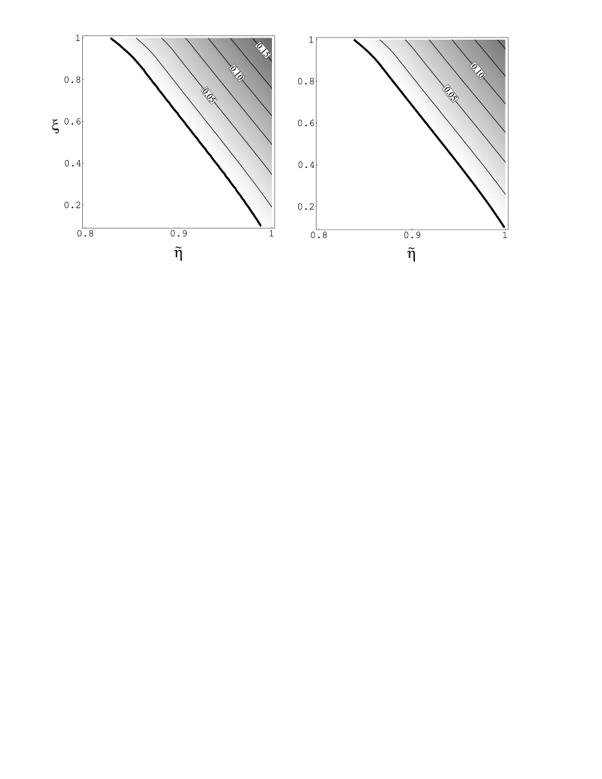
Figure 3: Maximized Clauser-Horne combination ${\cal CH}$ for a single photon divided at a beam splitter as a function of the overall losses $\tilde{\eta}$ and the mode mismatch $\xi$. Plots for noiseless detection $p_{\text{D}}=1$ (left) and with a dark-count rate $p_{\text{D}}=0.99$ (right). The thick lines represents the bound ${\cal CH}>0$ imposed by local-realistic theories.

In Fig. 3 we depict the optimum violation of the Clauser-Horne inequality as a function of the imperfection parameters $\tilde{\eta},\xi$, and $p_{D}$. As the dark count rates of silicon avalanche photodiodes are relatively low, we have chosen to study only two rather extreme values of the zero dark count probability: the ideal case $p_{D}=1$ and $p_{D}=0.99$ corresponding to $1\%$ dark count rate, which is well above what can be expected from modern detectors. It is seen that the difference between these two cases is rather minor. Instead, we have focused our attention on the detection efficiency $\tilde{\eta}$ and the mode mismatch $\xi$ as more critical parameters in a realistic situation. The graphs shown in Fig. 3 were obtained by selecting a $50\times 50$ grid in the plotted range of $\tilde{\eta}$ and $\xi$, and by performing the optimization procedure described above for each point of the grid. The contours in the plots have been drawn using interpolation, and the thick line separating the “nonlocal” region has been offset by $10^{-3}$ in order to avoid display of the effects of numerical errors.

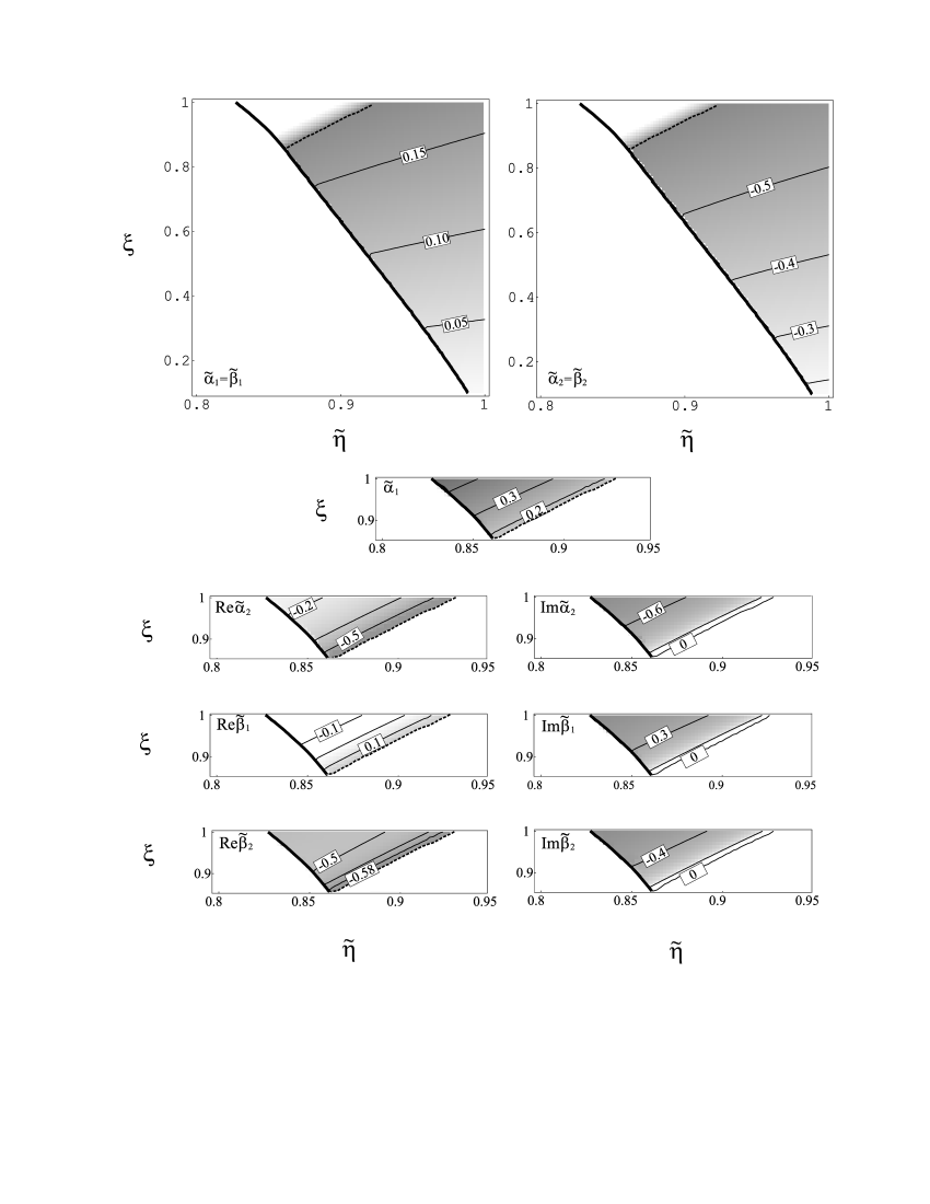
Figure 4: Coherent amplitudes maximizing violation of the Clauser-Horne inequality for the noiseless detection ($p_{\text{D}}=1$) as a function of the overall losses $\tilde{\eta}$ and the mode mismatch $\xi$. For the most of the area of violation it is sufficient to use just two real amplitudes (top $\tilde{\alpha}_{1}=\tilde{\beta}_{1}$ and $\tilde{\alpha}_{2}=\tilde{\beta}_{2}$. In a small triangular area separated by a dashed line the maximum violation is obtained for complex amplitudes, shown in the bottom seven figures.

It is seen that the maximum value of the Clauser-Horne combination, obtained for perfect detection efficiency and mode matching, lies above $0.15$. As expected, this value diminishes when $\tilde{\eta}$ and/or $\xi$ decrease, thus implying more imperfections in the setup. One can observe a clear trade-off between these two quantities: the worse the detection efficiency is, the better mode matching must be achieved in order to obtain a violation of the Clauser-Horne inequality. The minimum detection efficiency needed to observe the violation assuming perfect mode matching and zero dark counts is about $84\%$. In Fig. 4 we show the values of the coherent displacements that maximize the value of the Clauser-Horne combination. Numerical calculations have shown that in most of the area the maximum value is achieved by amplitudes that are real and pairwise equal: $\tilde{\alpha}_{1}=\tilde{\beta}_{1}$ and $\tilde{\alpha}_{2}=\tilde{\beta}_{2}$. These two values are depicted in Fig. 4(a). Only in a small triangular region in the parameter plane the situation becomes more complicated and the Clauser-Horne combination is maximized by displacement parameters with non-trivial imaginary parts. This region is shown in detail in seven graphs in Fig. 4(b).

VI Two-mode squeezed vacuum state

In this section we will discuss another possibility of using spontaneous parametric down-conversion as a source of entanglement for homodyne tests of Bell’s inequalities. The single-photon state discussed previously was obtained by conditional detection on the down-conversion output in the weak conversion regime, when the probability of generating simultaneously two or more photon pairs can be safely neglected. In a general case, the two-mode quantum state generated in spontaneous parametric down-conversion is of the form:

$$|\Phi\rangle=\frac{1}{\cosh r}\sum_{n=0}^{\infty}\tanh^{n}r\,|n\rangle_{A}|n\rangle_{B},$$ (36)

where $r$ is a squeezing parameter including information about the pump laser field, interaction time, thickness of the nonlinear crystal, etc. We have assumed here that the twin beams are generated in single spatio-temporal modes travelling towards directions $A$ and $B$.

The state given in Eq. (36) clearly exhibits entanglement in the Fock basis when the two modes are chosen as the separate subsystems. It is therefore interesting to study correlations between “photon silence” events on two spatially separated unbalanced homodyne detectors fed by the beams $A$ and $B$. We shall analyze whether such correlations are capable of violating the Clauser-Horne inequality (26). The relevant probabilities are calculated in Appendix, with the final results given by:

$$Q(\tilde{\alpha},\tilde{\beta}) = \frac{p_{\text{D}}^{2}}{1+\tilde{\eta}(2-\tilde{\eta})\sinh^{2}r}\exp\left[-\left(\frac{1+\tilde{\eta}\sinh^{2}r}{1+\tilde{\eta}(2-\tilde{\eta})\sinh^{2}r}+\frac{1-\xi}{\xi}\right)\tilde{\eta}(|\tilde{\alpha}|^{2}+|\tilde{\beta}|^{2})\right.$$ (37)

$$\left.+\frac{\tilde{\eta}^{2}\sinh r\cosh r}{1+\tilde{\eta}(2-\tilde{\eta})\sinh^{2}r}(\tilde{\alpha}\tilde{\beta}+\tilde{\alpha}^{*}\tilde{\beta}^{*})\right]$$

for the probability of a joint “photon silence” event and

$$Q(\tilde{\alpha}) = \ \frac{p_{\text{D}}}{1+\tilde{\eta}\sinh^{2}r}$$ (38)

$$\times\exp\left[-\left(\frac{1}{1+\tilde{\eta}\sinh^{2}r}+\frac{1-\xi}{\xi}\right)\tilde{\eta}|\tilde{\alpha}|^{2}\right]$$

describing the marginal probability of a zero count event on a single detector. Using these expressions we can build the combination (27) and check in what regime the Clauser-Horne inequality can be violated.

In order to find the optimal violation of the Clauser-Horne inequality we have followed the numerical procedure described in Sec. V. It is easy to note that the Clauser-Horne combination is invariant with respect to multiplying $\tilde{\alpha}_{1},\tilde{\alpha}_{2}$ and $\tilde{\beta}_{1},\tilde{\beta}_{2}$ by conjugate phase factors; we can therefore assume with no loss of generality that the amplitude $\tilde{\alpha}_{1}$ is purely real. An additional parameter that we have subjected to numerical optimization is the squeezing parameter $r$, as it should be possible to tune it rather easily by adjusting the intensity of the beam pumping the nonlinear medium.

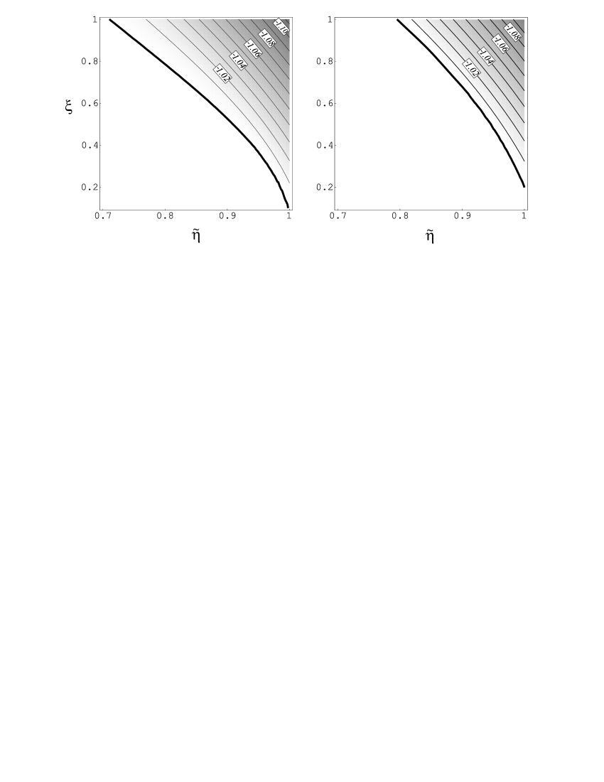
Figure 5: Optimal violation of the Clauser-Horne inequality for a squeezed state in the case of noiseless detection $p_{\text{D}}=1$ (left) and with a dark-count rate $p_{\text{D}}=0.99$ (right), as a function of the overall losses $\tilde{\eta}$ and the mode mismatch $\xi$.

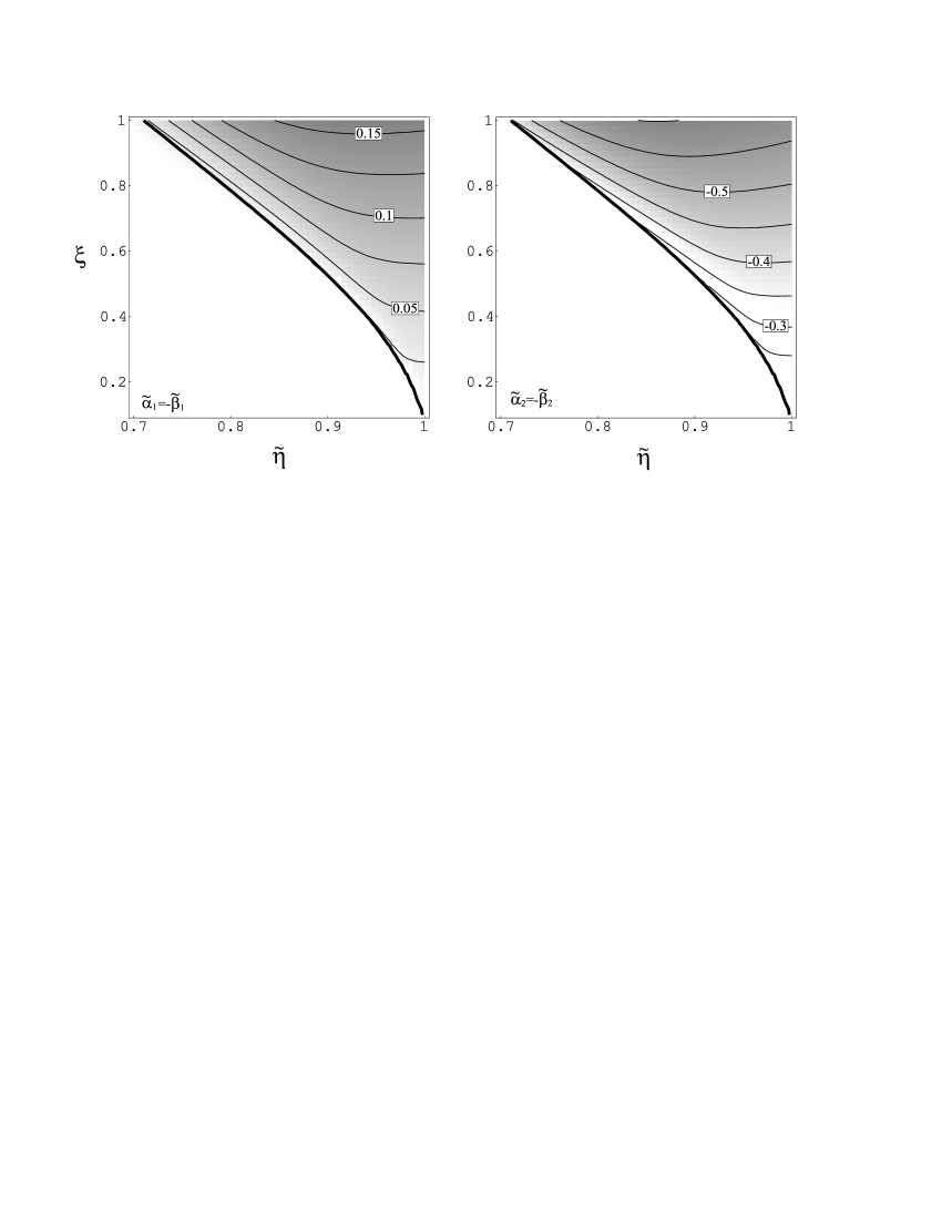
Figure 6: Coherent amplitudes maximizing violation of the Clauser-Horne inequality for the noiseless detection ($p_{\text{D}}=1$). It is sufficient to use just two real amplitudes $\tilde{\alpha}_{1}=-\tilde{\beta}_{1}$ and $\tilde{\alpha}_{2}=-\tilde{\beta}_{2}$.

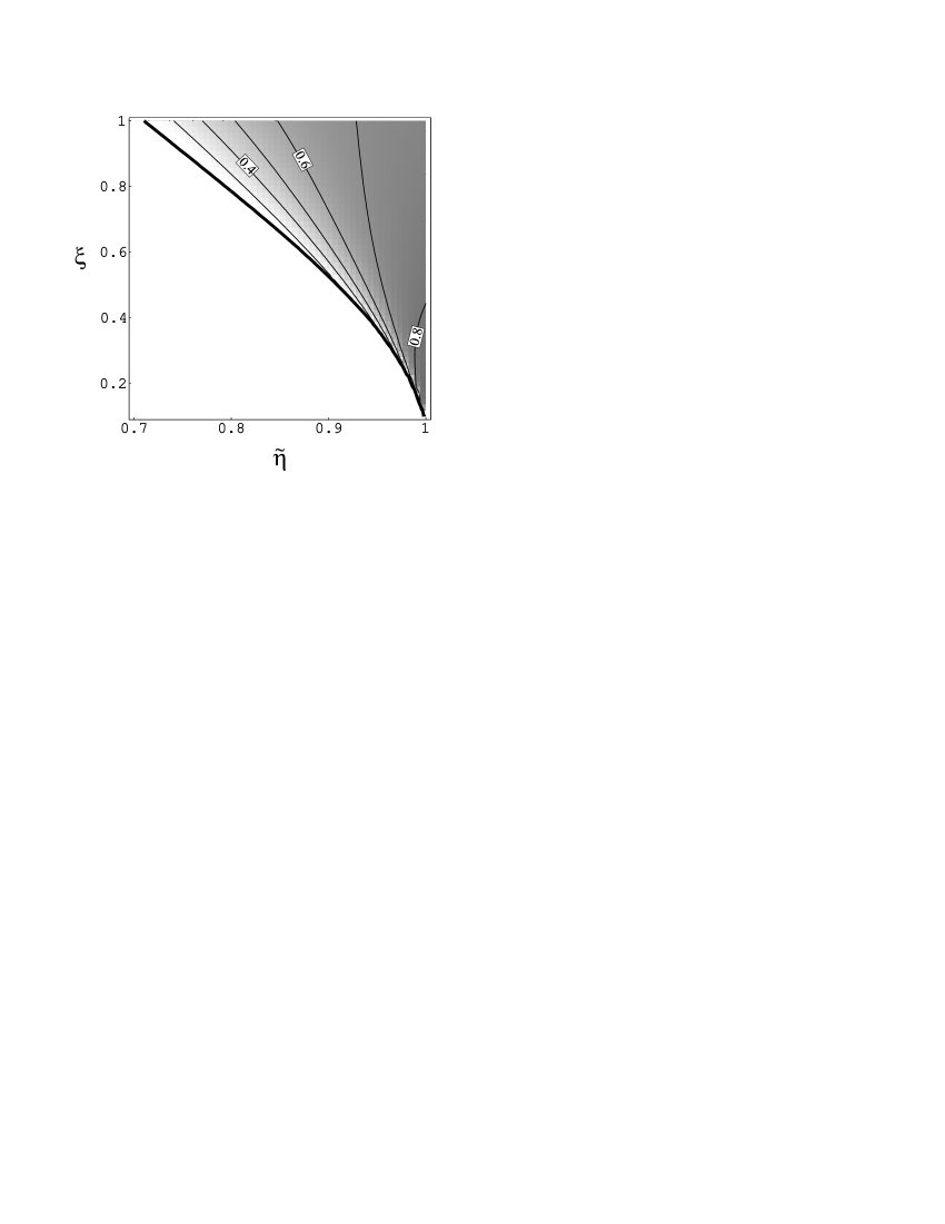
Figure 7: Squeezing parameter $r$ maximizing violation of the Clauser-Horne inequality for the noiseless detection ($p_{\text{D}}=1$).

In Fig. 5 we depict the minimized value of the Clauser-Horne combination as a function of the overall efficiency $\tilde{\eta}$ and mode matching $\xi$, for two values of the dark count rate: the ideal case $p_{D}=1$, and the 1% dark count probability corresponding to $p_{D}=0.99$. Once again one can observe a trade-off between the detection efficiency and the mode-matching. However, it is interesting to note that when a two-mode squeezed state is used as a source of entanglement, the minimum detection efficiency needed to violate the Clauser-Horne inequality is about $71\%$ in the case of perfect mode matching and absence of dark counts. For completeness, we show also the optimized values of the coherent displacements in Fig. 6 and the squeezing parameter in Fig. 7. We have found numerically that the Clauser-Horne combination is minimized by pairs of coherent displacements with opposite signs: $\tilde{\alpha}_{1}=-\tilde{\beta}_{1}$ and $\tilde{\alpha}_{2}=-\tilde{\beta}_{2}$. It is also interesting to note that optimal values of squeezing parameter are rather moderate, which means that only the first several terms in the Fock-basis expansion in Eq. (36) are relevant. This observation may be of experimental relevance, as good mode matching between the signal and local oscillator fields may be more difficult to achieve for strongly squeezed fields.

As it is well known, the two-mode squeezed vacuum state generated in spontaneous parametric down-conversion is described by a positive definite Wigner function. Quantum states of this form have been recalled on several occasions when discussing to what extent the quantum mechanical phase space formalism can serve as a local hidden-variable model. As this issue has generated some rather confusing comments in previous works, it is instructive to analyze from this point of view our homodyne scheme for testing Bell’s inequalities. For this purpose, let us use the Wigner formalism to rewrite the probability of a joint “photon silence” event $Q(\tilde{\alpha},\tilde{\beta})$ to a form that resembles a local hidden variable model:

$$Q(\tilde{\alpha},\tilde{\beta})=\int\text{d}^{2}\lambda_{1}\,\text{d}^{2}\lambda_{2}\;\rho(\tilde{\alpha};\lambda_{1})\rho(\tilde{\beta};\lambda_{2})W(\lambda_{1},\lambda_{2})$$ (39)

Here $\rho(\tilde{\alpha};\lambda_{1})$ and $\rho(\tilde{\beta};\lambda_{2})$ are Wigner representations of the observables corresponding to no-count events on the detectors $A$ and $B$, and $W(\lambda_{1},\lambda_{2})$ is the positive definite Wigner function of the state $|\Phi\rangle$. An easy calculation combining Eq. (29) with Eq. (41) from Appendix shows that $\rho(\tilde{\alpha};\lambda_{1})$ is explicitly given by

$$\rho(\tilde{\alpha};\lambda_{1})=\frac{2p_{D}}{2-\tilde{\eta}}\exp\left(-\frac{2\tilde{\eta}}{2-\tilde{\eta}}(\lambda_{1}-\tilde{\alpha})^{2}-\tilde{\eta}\frac{1-\xi}{\xi}|\tilde{\alpha}|^{2}\right)$$ (40)

with an analogous expression for $\rho(\tilde{\beta};\lambda_{2})$. In order to interpret $\rho(\tilde{\alpha};\lambda_{1})$ and $\rho(\tilde{\beta};\lambda_{2})$ as local realities that are defined by hidden variables $\lambda_{1}$ and $\lambda_{2}$, the expression given in Eq. (40) must be bounded between $0$ and $1$ as representing a local probability of a zero-count detection event. It is straightforward to see that the upper bound is in general violated: in the perfect case of $\tilde{\eta}=\xi=p_{D}=1$ the maximum value attained by $\rho(\tilde{\alpha};\lambda_{1})$ is equal to 2. Consequently, the Wigner representation given in Eq. (39) cannot be usually interpreted as a local hidden variable model for the “photon silence” events. It is clearly seen from the above example that positivity of the Wigner function describing a composite quantum system is in principle no obstacle to use it for demonstrating a violation of Bell’s inequalities. An equally important factor is whether the measured observables have a Wigner representation that can be interpreted in local realistic terms. Only when both these conditions are met, the detected correlation functions have to satisfy Bell’s inequalities.

VII Conclusions

In this paper, we presented a complete multimode theory of measuring quantum optical quasidistribution functions by photon counting. We demonstrated that by constructing a coherent field whose excited modes match pairwise the signal modes of interest, it is possible to scan point-by-point complete quasidistribution functions. Our analysis included effects of experimental imperfections, such as losses of the signal field, non-unit mode matching, and accidental dark counts.

As an interesting application of the developed formalism, we performed a feasibility study of using unbalanced homodyning for testing Bell’s inequalities. As a source of entanglement, we analyzed two states whose generation based on the process of spontaneous parametric down-conversion seems presently to be most practical. We found the range of experimental parameters that enable one to observe a violation of Bell’s inequalities without the standard postselection procedure. The minimum detection efficiency required for such a loophole-free test, in the absence of any other imperfections, is $84\%$ for a one-photon Fock state, and $71\%$ for a two-mode squeezed vacuum state. Especially the latter value seems to be within the reach of current technologies KwiaSteiPRA93 . Our calculations demonstrated a clear trade-off between two parameters describing experimental imperfections that are likely to determine the performance of a realistic setup: the detection efficiency and the mode mismatch. Such a trade-off is easily understandable: a natural way to improve the modal structure of the signal field is to perform spatio-temporal filtering, which, however, inevitably generates excess losses of the signal field. This effect underlines the need to develop sources of down-converted radiation with controlled spatio-temporal structure BanaURenOpL01 .

Though it does not affect directly tests of Bell’s inequalities, it is worthwhile to note that the optical states used in the scheme studied here do not share problems that are currently inherent to the standard down-conversion sources of polarization entangled states. In the latter case, the entangled photon pairs are generated only with a small probability per the time slot defined by the shape of the laser pulse pumping the nonlinear medium. Thus, the actual state of the produced light is given, up to the first order of the perturbation theory, by a small two-photon contribution superposed with a strong vacuum component KokBrauPRA00 . Within current technology it is not practical to perform a nondestructive test for the presence of photons thus selecting a priori the photon-pair term. Consequently experiments utilizing this type of entanglement, especially in quantum information processing applications, are usually based on the postselection of the detection events, and the strong vacuum component to the produced states is removed by retaining only the cases when a sufficient number of photons has been registered by the detectors. One might hope that this difficulty could be overcome by producing multiple photon pairs and using the methods of entanglement swapping and conditional detection to prepare the maximal polarization entanglement in the event-ready manner ZukoZeilPRL93 . However, there exists a rather general proof KokBrauPRA00 suggesting that this route is highly difficult, if not impossible, within presently available means. Practical realization of the states used in our study is not affected by these difficulties. The single photon state divided on a 50:50 beam splitter can be produced by conditional detection performed on the down-conversion output. Receiving signal from the trigger detector tells us unambiguously that the required single-photon state has been prepared with high fidelity. The preparation of the second state that was considered here, i.e. the two-mode squeezed vacuum state, does not require any postselection at all. The state produced from vacuum in the process of nondegenerate parametric down-conversion possess photon-number entanglement which is sufficient to violate Bell’s inequalities. Of course, this feature is not critical in tests of Bell’s inequalities which can rely validly on random sources of entangled photon pairs. However, the fact that we can reveal quantum nonlocality by performing dichotomic measurements on continuous-variable systems suggests that continous variable entanglement may be a useful resource in quantum information processing protocols based on binary logic, and our ability to produce it on demand could be its important advantage.

Appendix

Direct calculation of the quasidistributions of the state (36) is not as straightforward as in the case of single photon entangled with vacuum. Therefore we will calculate them using another method. First we will recall a useful property of a general, $M$-dimensional family of quasiprobability distributions: from any $s$-ordered quasidistribution one can calculate any other $s^{\prime}$-ordered one using the following integral formula:

$$W(\alpha_{1},\ldots,\alpha_{N};s^{\prime})=\left(\frac{2}{\pi(s-s^{\prime})}\right)^{M}\,\int\text{d}^{2}\beta_{1}\ldots\text{d}^{2}\beta_{M}\,\exp\left(-\frac{2}{s-s^{\prime}}\sum_{i=1}^{M}|\alpha_{i}-\beta_{i}|^{2}\right)W(\beta_{1},\ldots,\beta_{M};s).$$ (41)

A two-mode $Q$ function corresponding to the quasidistribution ordering parameter $s=-1$ can be very easily calculated for the NOPA state directly from the Fock representation:

$$W_{AB}(\gamma,\delta;-1)=\frac{1}{\pi^{2}}\mid\langle\gamma|\langle\delta|\Phi\rangle\mid^{2}=\frac{1}{\pi^{2}\cosh^{2}r}\exp\left[-|\gamma|^{2}-|\delta|^{2}+\tanh r\,\left(\gamma\delta+\gamma^{*}\delta^{*}\right)\right].$$ (42)

We will also need its marginal:

$$W_{A}(\gamma;-1)=\int\text{d}^{2}\delta\,W_{AB}(\gamma,\delta;-1)=\frac{1}{\pi\cosh^{2}r}\exp\left(-\frac{|\gamma|^{2}}{\cosh^{2}r}\right).$$ (43)

Inserting Eq. (42) into Eq. (41) specialized to the two-mode case with $M=2$ one easily obtains that:

$$W_{AB}\left(\tilde{\alpha},\tilde{\beta};-\frac{2-\tilde{\eta}}{\tilde{\eta}}\right) = \frac{\tilde{\eta}^{2}}{\pi^{2}(1+\tilde{\eta}(2-\tilde{\eta})\sinh^{2}r)}\exp\left(-\frac{\tilde{\eta}+\tilde{\eta}^{2}\sinh^{2}r}{1+\tilde{\eta}(2-\tilde{\eta})\sinh^{2}r}(|\tilde{\alpha}|^{2}+|\tilde{\beta}|^{2})\right.$$ (44)

$$\left.+\frac{\tilde{\eta}^{2}\sinh r\cosh r}{1+\tilde{\eta}(2-\tilde{\eta})\sinh^{2}r}(\tilde{\alpha}\tilde{\beta}+\tilde{\alpha}^{*}\tilde{\beta}^{*})\right)$$

Inserting the above formula into Eq. (29) yields the probability of the joint “photon silence” event given in Eq. (37). An analogous calculation yields the marginal single-mode quasidistribution function:

$$W_{A}\left(\tilde{\alpha};-\frac{2-\tilde{\eta}}{\tilde{\eta}}\right)=\frac{\tilde{\eta}}{\pi}\frac{1}{1+\tilde{\eta}\sinh^{2}r}\exp\left(-\frac{\tilde{\eta}\,|\tilde{\alpha}|^{2}}{1+\tilde{\eta}\sinh^{2}r}\right).$$ (45)

which after multiplying by the state-independent factors given in Eq. (30) gives the marginal probability of a no-count event given in Eq. (38).

References

- (1) For a review, see M. G. Raymer, Contemp. Phys. 38, 343 (1997); U. Leonhardt, Measuring the Quantum State of Light (Cambridge 1997).
- (2) P. G. Kwiat, K. Mattle, H. Weinfurter, A. Zeilinger, A. V. Sergienko and Y. H. Shih, Phys. Rev. Lett. 75, 4337 (1995); P. G. Kwiat, E. Waks, A. G. White, I. Appelbaum and P. H. Eberhard, Phys. Rev. A 60, R773 (1999); C. Kurtsiefer, M. Oberparleiter and H. Weinfurter, Phys. Rev. A 64, 023802 (2001).
- (3) D. Bouwmeester, J. W. Pan, K. Mattle, M. Eibl, H. Weinfurter and A. Zeilinger, Nature 390, 575 (1997); J. W. Pan, D. Bouwmeester, M. Daniell, H. Weinfurter and A. Zeilinger, ibid. 403, 515 (2000); A. Lamas-Linares, J. C. Howell and D. Bouwmeester, ibid. 412, 887 (2001).
- (4) P. G. Kwiat, A. J. Berglund, J. B. Altepeter and A. G. White, Science 290, 498 (2000); P. G. Kwiat, S. Barraza-Lopez, A. Stefanov and N. Gisin, Nature 409, 1014 (2001).
- (5) A. Furusawa, J. L. Sorensen, S. L. Braunstein, C. A. Fuchs, H. J. Kimble and E. S. Polzik, Science 282, 706 (1998).
- (6) W. P. Schleich, Quantum Optics in Phase Space (Wiley, 2001).
- (7) W. H. Zurek, Nature 412, 712 (2001).
- (8) D. T. Smithey, M. Beck, M. G. Raymer and A. Faridani, Phys. Rev. Lett. 70, 1244 (1993).
- (9) N. G. Walker and J. E. Caroll, Opt. Quant. Electron. 18, 355 (1986); N. G. Walker, J. Mod. Opt. 34, 15 (1987).
- (10) S. Wallentowitz and W. Vogel, Phys. Rev. A 53, 4528 (1996).
- (11) K. Banaszek and K. Wódkiewicz, Phys. Rev. Lett. 76, 4344 (1996).
- (12) K. Banaszek, C. Radzewicz, K. Wódkiewicz and J. S. Krasiński, Phys. Rev. A 60, 674 (1999).
- (13) K. Banaszek and K. Wódkiewicz, Phys. Rev. Lett. 82, 2009 (1999).
- (14) K. Banaszek and K. Wódkiewicz, Phys. Rev. A 58, 4345 (1998); Acta Phys. Slov. 49, 491 (1999).
- (15) P. Grangier, M. J. Potasek, and B. Yurke, Phys. Rev. A 38, 3132 (1988); S. M. Tan, D. F. Walls, and M. J. Collett, Phys. Rev. Lett. 66, 252 (1991).
- (16) J. Brendel, N. Gisin, W. Tittel and H. Zbinden, Phys. Rev. Lett. 82, 2594 (1999); W. Tittel, J. Brendel, H. Zbinden and N. Gisin, ibid. 84, 4737 (2000).
- (17) A. Kuzmich, I. A. Walmsley and L. Mandel, Phys. Rev. Lett. 85, 1349 (2000).
- (18) H. P. Yuen and J. H. Shapiro, IEEE Trans. Inf. Theory IT-26, 78 (1980); M. G. Raymer, J. Cooper, H. J. Carmichael, M. Beck and D. T. Smithey, J. Opt. Soc. Am. B 12, 1801 (1995).
- (19) A. I. Lvovsky, H. Hansen, T. Aichele, O. Benson, J. Mlynek and S. Schiller, Phys. Rev. Lett. 87, 050402 (2001).
- (20) S. L. Braunstein, Nature 394, 47 (1998); S. Lloyd and S. L. Braunstein, Phys. Rev. Lett. 82, 1784 (1999).
- (21) Z.-B. Chen, J.-W. Pan, G. Hou and Y.-D. Zhang, Phys. Rev. Lett. 88, 040406 (2002).
- (22) J. W. Wu, Phys. Rev. A 61, 022111 (2000).
- (23) Z. Kis, T. Kiss, J. Janszky, P. Adam, S. Wallentowitz and W. Vogel, Phys. Rev. A 59, R39 (1999).
- (24) A. Gilchrist, P. Deuar and M. D. Reid, Phys. Rev. Lett. 80, 3169 (1998).
- (25) A. Dragan and K. Banaszek, Phys. Rev. A 63, 062102 (2001).
- (26) W. Vogel, D.-G. Welsch and S. Wallentowitz, Quantum Optics: An Introduction, 2nd Ed. (Wiley, 2001).
- (27) K. E. Cahill and R. J. Glauber, Phys. Rev. 177, 1857 (1969).
- (28) K. Banaszek and K. Wódkiewicz, J. Mod. Opt. 44, 2441 (1997).
- (29) J. S. Kim, S. Takeuchi, Y. Yamamoto, and H. H. Hogue, Appl. Phys. Lett. 74, 902 (1999).
- (30) P. Kok and S. L. Braunstein, Phys. Rev. A 63, 033812 (2001).
- (31) K. Banaszek and I. A. Walmsley, preprint quant-ph/0206162.
- (32) J. F. Clauser and M. A. Horne , Phys. Rev. D 10, 526 (1974).
- (33) D. M. Greenberger, M. A. Horne and A. Zeilinger, in Quantum Interferometry II, edited by F. De Martini, G. Deuardo and Y. Shih (VCH, Weinheim 1997).
- (34) L. Hardy, Phys. Rev. Lett. 73, 2279 (1994); L. Vaidman, ibid. 75, 2063 (1995); D. M. Greenberger, M. A. Horne and A. Zeilinger, ibid. 75, 2064 (1995); L. Hardy, ibid. 75, 2065 (1995).
- (35) W. H. Press, S. A. Teukolsky, W. T. Vetterling, and Brian P. Flannery, Numerical Recipes, 2nd edition (Cambridge University Press, 1992), Sec. 10.4.
- (36) P. G. Kwiat, A. M. Steinberg, R. Y. Chiao, P. H. Eberhard, and M. D. Petroff, Phys. Rev. A 48, R867 (1993).
- (37) K. Banaszek, A. B. U’Ren, and I. A. Walmsley, Opt. Lett. 26, 1367 (2001).
- (38) P. Kok and S. L. Braunstein, Phys. Rev. A 62, 064301 (2000).
- (39) M. Żukowski, A. Zeilinger, M. A. Horne and A. K. Ekert, Phys. Rev. Lett. 71, 4287 (1993).