The Effect of Stochastic Noise on Quantum State Transfer

Abstract

We consider the effect of classical stochastic noise on control laser pulses used in a scheme for transferring quantum information between atoms, or quantum dots, in separate optical cavities via an optical connection between cavities. We develop a master equation for the dynamics of the system subject to stochastic errors in the laser pulses, and use this to evaluate the sensitivity of the transfer process to stochastic pulse shape errors for a number of different pulse shapes. We show that under certain conditions, the sensitivity of the transfer to the noise depends on the pulse shape, and develop a method for determining a pulse shape that is minimally sensitive to specific errors.

I Introduction

The ability to transfer a quantum state from one system to another will be a useful tool in the future of quantum information, both for quantum communication and for building large quantum computers from smaller components. Various schemes have been proposed for transferring quantum states Cirac et al. (1997); Pellizzari (1997); van Enk et al. (1997b, a, 1999); Virjen and Yablonovitch (2000); Duan et al. (2001), some of which are based on teleportation and entanglement purification. Others are more direct, having a quantum channel (typically an optical fiber) connecting the two systems, and classical control pulses applied to each system ensure that emission from the first system and absorption by the second are perfect.

Over long distances, it appears that protocols based on teleportation and purification are necessarily more efficient than direct schemes Duan et al. (2001), but over short distances (e.g. for interconnects between quantum components), the more direct method, first proposed by Cirac et al. Cirac et al. (1997), may be practical, and is probably easier to implement since it does not require quantum measurement. The scheme by Cirac et al. Cirac et al. (1997) implements quantum state transfer from one atom located inside an optical cavity to another atom in a separate but connected cavity, mediated by Raman transitions via an atomic state (outside the computational basis) as well as cavity and external photons, and is controlled by laser pulses incident on each atom. The transfer is therefore subject to amplitude and phase errors in the control pulses.

The idea Cirac et al. (1997) is also applicable to single-electron spin based systems in semiconductors, with additional uses such as spin measurement Imamoḡlu et al. (1999); Imamoḡlu (2000), and as a controllable source of decoherence for initial state preparation. The intermediate state required for spin-flip Raman transitions between single electron spin states is a state known as a trion Imamoḡlu et al. (1999); Imamoḡlu (2000). This state is a bound state of two electrons and a single hole, and couples to the single electron spin states via $x$- and $y$-polarised light. Physically, this corresponds to the optical excitation of an exciton which may form a bound state with the electron, very much akin to an H^- complex. Trion states have been observed experimentally in GaAs Shields et al. (1995, 2001), and are relatively long lived, and so the scheme has the potential to be realised in semiconductor systems.

In this paper we present an analysis of the effect of two possible types of stochastic error in control pulses, and consider a method for reducing the sensitivity of the pulse to such errors. Our results show that it is possible to design pulse shapes that reduce the sensitivity of the transfer process to certain sources of errors in the pulse. We give a short account of the applicability of this scheme to a semiconductor device.

In section II we briefly review the proposal for quantum state transfer given by Cirac et al. (1997) and give a new analytic form for a laser control pulse shape that implements quantum state transfer. In section III we formulate a master equation for the transfer subject to stochastic errors in the control pulse, and use the master equation to compute the sensitivity of the transfer process to such errors. In section IV we present a procedure to optimise the pulse shape to reduce the sensitivity of the transfer to control pulse errors. We then finish with some conclusions.

II Quantum State Transfer

II.1 Review of proposal

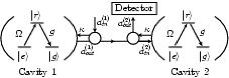
Figure 1: Schematic arrangement of cavity and three level system. The small circles represent Faraday isolators so the forward and reverse propagating paths are distinguishable. Adapted from Cirac et al. Cirac et al. (1997).

In Cirac et al.’s proposal for quantum state transfer, Cirac et al. (1997), two 3-level systems (atoms, in the original proposal) are located inside separate optical cavities, as illustrated in Fig. 1, with the left atom starting in an arbitrary superposition of its lower levels, $|\psi\rangle=c_{g}|g\rangle+c_{e}|e\rangle$, and the right atom in the state $|g\rangle$. The objective of quantum state transfer is then to transfer the state $|\psi\rangle$ from atom 1 to atom 2 by applying suitable laser pulses to each atom. This may be expressed as

$$|\psi\rangle_{1}|g\rangle_{2}\otimes|0\rangle_{1}|0\rangle_{2}\rightarrow|g\rangle_{1}|\psi\rangle_{2}\otimes|0\rangle_{1}|0\rangle_{2},$$ (1)

where the subscripts indicate the atom/cavity system. The term $|0\rangle_{j}$ is cavity $j$’s photon state in the number basis, and is the vacuum state at the start and end of the process.

In the case that the detuning between the laser frequency and the atomic transition from $|g\rangle$ to $|e\rangle$, $\omega_{L}-\omega_{0}$, is larger than all other frequencies in the problem, one can write a Hamiltonian for each atom-cavity system, labeled $j=1,2$, from which the upper level $|r\rangle$ is adiabatically eliminated,

$$\hat{H}_{j}(t)/\hbar=\frac{\Omega_{j}(t)^{2}}{4(\omega_{L}-\omega_{0})}|e\rangle_{jj}\langle e|-ig_{j}(t)(e^{i\phi_{j}(t)}|e\rangle_{jj}\langle g|\hat{a}_{j}-\mathrm{H.c}).$$ (2)

Here, $\Omega_{j}(t)=2\bm{\mu}_{er}\cdot\bm{\varepsilon}E_{j}(t)/\hbar$ is the classical Rabi frequency of the atom-laser system and $g(t)=g\Omega(t)/(\omega_{L}-\omega_{0})$ is the effective coupling strength between state $|g\rangle$ and $|e\rangle$, and is proportional to $E_{j}(t)$, the amplitude of the laser electric field, which we will use to control the transfer. We have also made the following definitions: $\hat{a}_{j}$ is cavity $j$’s photon creation operator, $g$ is the cavity-atom coupling strength, $\bm{\mu}_{er}$ is the dipole matrix element between $|e\rangle$ and $|r\rangle$, $\bm{\varepsilon}$ is the laser polarisation, and $\phi_{j}(t)$ is the phase of the laser. In deriving this equation, there is an assumption that the laser frequency is detuned from the cavity mode , $\omega_{c}$, nearest the transition, by an amount $\omega_{l}-\omega_{c}=g^{2}/(\omega_{L}-\omega_{0})$, which is the ac-Stark shift of the state $|g\rangle_{j}$ in the electric field of the laser.

Following the original proposal by Cirac et al. Cirac et al. (1997), the transfer is made to be unidirectional and is constrained by the requirement that the photodetector, indicated in Fig. 1, never registers a photon. The entire system is then an open quantum system, and is described equivalently by a quantum master equation, or a quantum trajectory punctuated by quantum jumps Gardiner and Zoller (2000). Since it will become important for the later development of this paper, we summarise now some important points from Cirac et al., who adopt the quantum trajectories approach to the problem. The non-Hermitian effective Hamiltonian that describes the evolution of the open system in between jumps is $\hat{H}_{\mathrm{eff}}=\hat{H}_{1}+\hat{H}_{2}-i\kappa(\hat{a}_{1}^{\dagger}\hat{a}_{1}+\hat{a}_{2}^{\dagger}\hat{a}_{2}+2\hat{a}_{2}^{\dagger}\hat{a}_{1})$, where $\kappa$ is the cavity leakage rate and the jump operator is $\hat{c}=\hat{a}_{1}+\hat{a}_{2}$. In the language of quantum trajectories, the system state vector evolves under the Schrödinger equation with the effective Hamiltonian $H_{\mathrm{eff}}$. This Hamiltonian does not increase the total excitation number of the system, so we write the state vector as

$$|\psi(t)\rangle=c_{g}|gg\rangle|00\rangle+c_{e}\left\{\alpha_{1}(t)e^{-i\phi_{1}(t)}|eg\rangle|00\rangle+\alpha_{2}(t)e^{-i\phi_{2}(t)}|ge\rangle|00\rangle\vphantom{\frac{\beta_{s}(t)}{\sqrt{2}}}\right.+\left.|gg\rangle\left(\frac{\beta_{s}(t)}{\sqrt{2}}(|01\rangle+|10\rangle)+\frac{\beta_{a}(t)}{\sqrt{2}}(|01\rangle-|10\rangle)\right)\right\}.$$ (3)

The initial conditions and final configuration (for a successful transfer) are

$$\alpha_{1}(-\infty)=1,\phi_{1}(-\infty)=0\textrm{ and }\alpha_{2}(+\infty)=1,\phi_{2}(+\infty)=0.$$ (4)

we refer to the condition at $t=+\infty$ as the zero-jump condition, which holds as long as as $\hat{c}|\psi(t)\rangle=0$ for all $t$, and this requires that

$$\beta_{s}(t)=0.$$ (5)

If we choose the phase of the laser to vary with time according to $\dot{\phi}_{j}(t)=\Omega_{j}(t)^{2}/(4(\omega_{L}-\omega_{0}))$ then all $\phi_{j}$ dependence factorises out of the Schrödinger, resulting in the linearly independent evolution equations

$$\dot{\alpha}_{1}(t) = g_{1}(t)\beta_{a}(t)/\sqrt{2},$$ (6a)

$$\dot{\alpha}_{2}(t) = -g_{2}(t)\beta_{a}(t)/\sqrt{2},$$ (6b)

$$\dot{\beta}_{s}(t) = g_{1}(t)\alpha_{1}(t)/\sqrt{2}+g_{2}(t)\alpha_{2}(t)/\sqrt{2}+\kappa\beta_{a}(t).$$ (6c)

Finally, the normalisation condition for the state vector requires that

$$|\alpha_{1}(t)|^{2}+|\alpha_{2}(t)|^{2}+|\beta_{s}(t)|^{2}+|\beta_{a}(t)|^{2}=1.$$ (7)

We could also write an evolution equation for $\beta_{a}$, however this is the same equation as obtained by differentiating Eq. (7) with respect to time, and then substituting Eqs. (6a) and (6b), so is not linearly independent.

There are thus only five independent equations, Eqs. (5) through (7), but six unknowns, $\alpha_{1},\alpha_{2},\beta_{s},\beta_{a},g_{1}$ and $g_{2}$, and so there is no unique solution that satisfies the requirements of quantum state transfer. There is a notable symmetry in the evolution equations and the initial and final states which is that if the cavity labels $j=1,2$ are exchanged and time is reversed, i.e. $1\leftrightarrow 2$ and $t\rightarrow-t$, then they are recovered, so long as $g_{2}(t)=g_{1}(-t)$, which is referred to as the symmetric pulse condition. Under this condition, Cirac et al. Cirac et al. (1997) present a method for generating pulse shapes that satisfy the requirements of quantum state transfer. This procedure is as follows:

1. Select $g_{1}(t)$ for $t\geq 0$.

2. Solve Eq. (6a) and a reduced form of Eq. (6c): $\dot{\beta}_{a}(t)=-g_{1}(t)\beta_{a}(t)/\sqrt{2}-\kappa g_{1}(t)\alpha_{1}(t)$, subject to the initial conditions $\alpha_{1}(0)=\kappa/\sqrt{2(g_{1}(0)^{2}+\kappa^{2})}$ and $\beta_{a}(0)=-\sqrt{1-2\alpha_{1}(0)}$.

3. Define $g_{1}(t)=-(\sqrt{2}\kappa\beta_{a}(|t|)+g_{1}(|t|)\alpha_{1}(|t|))/\alpha_{2}(|t|)$ for $t<0$.

Then $g_{1}(t)$ is defined at all times, and as long as $g_{1}(+\infty)>0$, this pulse shape will satisfy the requirements of quantum state transfer. Cirac et al. Cirac et al. (1997) present a particular solution to the equations, which they show accomplishes the transfer successfully.

We make the point that if $g_{1}(t)\rightarrow 0$ as $t\rightarrow+\infty$ the method doesn’t guarantee a successful transfer pulse shape, but it does allow us to evaluate the success of a transfer based only on knowledge of $g_{1}(t)$ for $t\geq 0$, subject to the presumption that $g_{1}(t):t<0$ is determined from $g_{1}(t):t\geq 0$, according to the above procedure.

II.2 Alternate solution method

Using Eqs. (6a) and (6b) to replace $g_{1}(t)$ and $g_{2}(t)$ in Eq. (6c), along with the zero jump condition, Eq. (5), as well as the normalisation condition Eq. (7) results in the following reduced non-linear equation for $\alpha_{1}(t)$ and $\alpha_{2}(t)$,

$$\frac{d}{dt}\left(\frac{\alpha_{1}(t)^{2}-\alpha_{2}(t)^{2}}{2}\right)+\kappa(1-\alpha_{1}(t)^{2}-\alpha_{2}(t)^{2})=0.$$ (8)

Thus, another approach to finding a suitable pulse shape is to invent another equation depending on $\alpha_{1}(t)$ and $\alpha_{2}(t)$ (i.e. $f(\alpha_{1}(t),\alpha_{2}(t))=0$) consistent with Eqs. (4) and (7) and then solve this equation and Eq. (8) to find $\alpha_{1}(t)$ and $\alpha_{2}(t)$, from which we can calculate the other functions.

We can motivate an example of this method by making $g_{1}(t)=g_{2}(t)$, so that pulses on each atom are the same. We then divide Eq. (6a) by Eq. (6b), to find $\dot{\alpha}_{1}(t)=-\dot{\alpha}_{2}(t)$, and taking account of the initial condition, Eq. (4), we find that $\alpha_{1}(t)+\alpha_{2}(t)=1$, which is of the form $f(\alpha_{1}(t),\alpha_{2}(t))=0$, and is consistent with Eqs. (4) and (7). Thus we can use this as a second equation, along with Eq. (8) to solve for $\alpha_{1}(t)$ and $\alpha_{2}(t)$. By substituting for $\alpha_{2}(t)$ in Eq. (8), we find that $\alpha_{1}(t)$ satisfies

$$\dot{\alpha}_{1}(t)+2\kappa(\alpha_{1}(t)-\alpha_{1}(t)^{2})=0.$$ (9)

There are two solutions to this equation, $\alpha_{1}(t)=(1\pm e^{2\kappa t})^{-1}$, however one is unphysical since it diverges at $t=0$ (violating the normalisation condition). The physical solution is $\alpha_{1}(t)=(1-\tanh(\kappa t))/2$, and from this we can determine all the other quantities to be

$$\alpha_{2}(t) = \alpha_{1}(-t)=(1+\mathrm{tanh}(\kappa t))/2,$$ (10a)

$$\beta_{a}(t) = -\mathrm{sech}(\kappa t))/\sqrt{2},$$ (10b)

$$g_{1}(t) = g_{2}(t)=\kappa\,\mathrm{sech}(\kappa t)\vphantom{\frac{\mathrm{sech}(\kappa t)}{\sqrt{2}}}.$$ (10c)

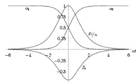
Figure 2: Plot of the quantities given by Eqs. (10a) to (10c).

Notably, this solution has the property that $g_{1}(t)\rightarrow 0$ as $t\rightarrow\infty$, and it also satisfies the symmetric pulse condition, $g_{2}(t)=g_{1}(-t)$, so is a member of the class of solutions generated by the method of Cirac et al. Cirac et al. (1997). We now have two solutions out of an infinite range of possible ones (i.e. the solution presented in Cirac et al. (1997), and the one above), which we will compare in later sections.

III Stochastic Noise in Laser Pulse

Having presented an alternate pulse shape to accomplish quantum state transfer, we now use the two solutions, that in Cirac et al. Cirac et al. (1997) and in this paper, as test cases for evaluating the effect of stochastic noise in the laser pulses on the fidelity of the transfer. We reformulate the problem in terms of a quantum master equation, as opposed to that of quantum trajectories van Enk et al. (1997b, a); Cirac et al. (1997), since we will eventually take averages over an ensemble of noise realisations, which must be done with respect to the density matrix rather than the state vector.

III.1 Master Equation

Since the process of information transfer is one-way, we adopt the cascaded quantum system approach, described in the text by Gardiner and Zoller Gardiner and Zoller (2000), to derive a master equation. The quantum master equation for the cascaded system here is given by

$$\dot{\rho}=-\frac{i}{\hbar}\left[\hat{H}_{1}(t)+\hat{H}_{2}(t),\rho\right]+\kappa\mathscr{L}\{\rho\},$$ (11a)

$$\begin{split}\mathscr{L}\{\rho\}=&2\hat{a}_{1}\rho\hat{a}_{1}^{\dagger}-\hat{a}_{1}\hat{a}_{1}^{\dagger}\rho-\rho\hat{a}_{1}\hat{a}_{1}^{\dagger}\\ &+2\hat{a}_{2}\rho\hat{a}_{2}^{\dagger}-\hat{a}_{2}\hat{a}_{2}^{\dagger}\rho-\rho\hat{a}_{2}\hat{a}_{2}^{\dagger}\\ &-2\{[\hat{a}_{2}^{\dagger},\hat{a}_{1}\rho]+[\rho\hat{a}_{1}^{\dagger},\hat{a}_{2}]\},\end{split}$$ (11b)

where $\rho$ is the system density matrix. Subsequently, we leave out explicit time dependence notation from the Hamiltonians, $H_{1}$ and $H_{2}$, unless required for clarity. In lieu of writing out all 25 coupled, first-order differential equations arising from the master equation, we give a schematic representation of the coupling between elements of the density matrix in Fig. 3, where arrows indicate the direction of the coupling.

$$\begin{matrix}|g0g0\rangle\\ \\ |e0g0\rangle\\ |g1g0\rangle\\ \\ |g0e0\rangle\\ |g0g1\rangle\end{matrix}\hskip 28.45274pt\begin{bmatrix}\begin{bmatrix}\bm{\rho}_{1,1}\end{bmatrix}&&\begin{bmatrix}\bm{\rho}_{1,2}&\rho_{1,3}\end{bmatrix}&\rightarrow&\begin{bmatrix}\rho_{1,4}&\rho_{1,5}\end{bmatrix}\\ &\nwarrow&&&\\ \begin{bmatrix}\bm{\rho}_{2,1}\\ \rho_{3,1}\end{bmatrix}&&\begin{bmatrix}\bm{\rho}_{2,2}&\rho_{2,3}\\ \rho_{3,2}&\rho_{3,3}\end{bmatrix}&\rightarrow&\begin{bmatrix}\rho_{2,4}&\rho_{2,5}\\ \rho_{3,4}&\rho_{3,5}\end{bmatrix}\\ \downarrow&&\downarrow&&\downarrow&\\ \begin{bmatrix}\rho_{4,1}\\ \rho_{5,1}\end{bmatrix}&&\begin{bmatrix}\rho_{4,2}&\rho_{4,3}\\ \rho_{5,2}&\rho_{5,3}\end{bmatrix}&\rightarrow&\begin{bmatrix}\rho_{4,4}&\rho_{4,5}\\ \rho_{5,4}&\rho_{5,5}\end{bmatrix}\end{bmatrix}$$

Figure 3: Structure of relationships between density matrix elements arising from Eq. (11a), with respect to the basis $\mathcal{B}$, which is indicated on the left. Elements within each sub-matrix are mutually coupled. Arrows indicate the direction of coupling between the sub-matrices, so for instance $\dot{\rho}_{5,5}$ depends on $\rho_{3,5}$, but not vice-versa, i.e. derivatives are placed at the arrow head, for example the equation for $\dot{\rho}_{{5,5}}$ is $\dot{\rho}_{5,5}={g_{2}}(t)\left(\rho_{4,5}+\rho_{5,4}\right)-2\kappa\left(\rho_{3,5}+\rho_{5,3}+\rho_{5,5}\right)$. The arrows therefore indicate the flow of information, from the states with a single excitation in the left cavity to single excitation in the right cavity, but not in reverse, as determined by the one-way requirement used to formulate the equations. The bold elements are those that may be non-zero at $t=-\infty$, and are given by $|\psi\rangle\langle\psi|$.

From this schematic representation we can see how the equations ensure that information does flow unidirectionally from the left cavity to the right. The initial condition for this master equation is simply

$$\rho(-\infty)=(|\psi\rangle_{1}|g\rangle_{2}|00\rangle)({}_{1}\langle\psi|_{2}\langle g|\langle 00|).$$ (12)

For future reference, if a matrix representation of an operator is given, it will be expressed with respect to the basis $\mathcal{B}=\{|g0g0\rangle,|e0g0\rangle,|g1g0\rangle,|g0e0\rangle,|g0g1\rangle\}$, where the state vector notation represents the state of the left atom, left photon number, right atom and right photon number in order. The solutions we are interested in will be those for which quantum state transfer has been successfully implemented, so

$$\rho(+\infty)=(|g\rangle_{1}|\psi\rangle_{2}|00\rangle)({}_{1}\langle g|_{2}\langle\psi|\langle 00|).$$ (13)

We will use the notation $\rho_{0}(t)$ to indicate any solution to the noiseless master equation, Eq. (11a), which satisfies both Eqs. (12) and (13). For an arbitrary time $t$, $\rho_{0}(t)$ will depend on the pulse shape, nevertheless all permissible solutions will agree at $t=\pm\infty$. Of course, for those pulses that do satisfy the requirement of quantum state transfer, the master equation will give the same result as solving the quantum trajectory equations, Eq. (6).

III.2 Adding Stochastic Noise

We add the effect of stochastic noise in the pulse shapes to the dynamics of the problem, and so we follow a similar development to that presented in recent work Budini (2001); Wellard and Hollenberg (2001). We assume that for each realisation of a transfer attempt, the actual classical laser pulse, $\tilde{g}_{j}(t)$, applied to atom $j$ is perturbed from the desired shape according to $\tilde{g}_{j}(t)=g_{j}(t)+\xi_{j}(t)\Delta g_{j}(t)$, where $\xi_{j}(t)$ is a stochastic function of time, and $\Delta g_{j}(t)$ is some function which will depend on the origin of the stochastic error (i.e. noise), and is considered to be small. For instance, if the noise is associated with fluctuations in the amplitude of the pulse, then $\Delta g_{j}(t)=g_{j}(t)$, so that $\tilde{g}_{j}(t)=(1+\xi_{j}(t))g_{j}(t)$, and if it is associated with errors in timing between the pulses applied to the two cavities then $\Delta g_{j}(t)=\dot{g_{j}}(t)$, both of which we consider later. This modifies the atom-cavity Hamiltonian from that with an ideal pulse, which to first order in $\xi_{j}(t)$ is

$$\hat{H}_{j}(t)\rightarrow\hat{H}_{j}(t)+\xi_{j}(t)\hat{h}_{j}(\Delta g_{j}(t)).$$ (14)

The operator $\hat{h}_{j}$ is Hermitian and depends on $\Delta g_{j}(t)$.

With the modified Hamiltonian given in Eq. (14), the master equation reads

$$\dot{\rho}=-\frac{i}{\hbar}\left[\hat{H}_{1}+\xi_{1}(t)\hat{h}_{1}(t)+\hat{H}_{2}+\xi_{2}(t)\hat{h}_{2}(t),\rho\right]+\kappa\mathscr{L}\{\rho\},$$ (15)

which we formally integrate on both sides to find $\rho(t)$ and substitute back into the right-hand side (RHS) of the equation, to generate the second order term in the Dyson series. We then take averages over an ensemble of noise realisations, and assuming the one-time correlation terms have zero mean, i.e. $\langle\xi_{j}(t)\rangle=0,$ we arrive at the result

$$\begin{split}\langle\dot{\rho}(t)\rangle=&-i/\hbar\left[H_{1}+H_{2},\langle\rho(t)\rangle\right]+\kappa\mathscr{L}\{\langle\rho(t)\rangle\}\\ &+(i/\hbar)^{2}\left(\left[\hat{h}_{1},\int_{-\infty}^{t}dt^{\prime}\langle\left[\xi_{1}(t)\xi_{1}(t^{\prime})\hat{h}_{1}(t^{\prime}),\rho(t^{\prime})\right]\rangle\right]+\left[\hat{h}_{2},\int_{-\infty}^{t}dt^{\prime}\langle\left[\xi_{2}(t)\xi_{2}(t^{\prime})\hat{h}_{2}(t^{\prime}),\rho(t^{\prime})\right]\rangle\right]\right.\\ &\hphantom{+(i/\hbar)^{2}}+\left.\left[\hat{h}_{1},\int_{-\infty}^{t}dt^{\prime}\langle\left[\xi_{1}(t)\xi_{2}(t^{\prime})\hat{h}_{2}(t^{\prime}),\rho(t^{\prime})\right]\rangle\right]+\left[\hat{h}_{2},\int_{-\infty}^{t}dt^{\prime}\langle\left[\xi_{2}(t)\xi_{1}(t^{\prime})\hat{h}_{1}(t^{\prime}),\rho(t^{\prime})\right]\rangle\right]\right).\end{split}$$ (16)

We write the averaged solution to the noisy master equation, Eq. (16), as a correction to $\rho_{0}(t)$, the density matrix in the absence of noise,

$$\langle\rho(t)\rangle=\rho_{0}(t)+\epsilon_{1}\Delta\rho_{1}(t)+\epsilon_{2}\Delta\rho_{2}(t),$$ (17)

where $\epsilon_{j}$ is a measure of the (small) variance of the noise on laser pulse $j$, and will appear as a coefficient in the two-time correlation function $\langle\xi_{j}(t)\xi_{j}(t^{\prime})\rangle$. In the case that the stochastic terms on each pulse are uncorrelated with one another, $\langle\xi_{1}(t)\xi_{2}(t^{\prime})\rangle=0$, which we will hereafter assume, we can substitute Eq. (17) into Eq. (16) and use Eq. (11a) to derive two independent master equations for the first order (in $\epsilon_{j}$) correction terms $\Delta\rho_{1}(t)$ and $\Delta\rho_{2}(t)$,

$$\begin{split}\dot{\Delta\rho_{j}}=&-i/\hbar\left[\hat{H}_{1}+\hat{H}_{2},\Delta\rho_{j}\right]+\kappa\mathscr{L}\{\Delta\rho_{j}\}\\ &+(i/\hbar)^{2}\left[\hat{h}_{j},\int_{-\infty}^{t}dt^{\prime}\left[\frac{\langle\xi_{j}(t)\xi_{j}(t^{\prime})\rangle}{\epsilon_{j}}\hat{h}_{j}(t^{\prime}),\rho_{0}(t^{\prime})\right]\right].\end{split}$$ (18)

The quantity $\epsilon_{j}\Delta\rho_{j}(t)$ is therefore interpreted as a correction to the noiseless density matrix due to stochastic errors in pulse $j$. We note that the homogeneous part of the above equation is the same as the original noiseless master equation, Eq. (11a), but it now has an inhomogeneous driving term that depends on the solution to the noiseless equation, $\rho_{0}(t)$. We are interested in errors in the density matrix associated with stochastic errors in the pulse shape, so we assume that the initial state of the density matrix can be prepared exactly, i.e $\Delta\rho_{j}(-\infty)=0$. The solution to equation Eq. (11a) as $t\rightarrow\infty$ is determined by Eq. (13), but the solution to Eq. (18) is not constrained and may depend on both $g_{j}(t)$ and $\Delta g_{j}(t)$.

In numerical investigations of the error, we assume that the initial state of the left atom is $|\psi\rangle=|e\rangle$, so that the only non-zero matrix element is $\langle e0g0|\rho_{0}(-\infty)|e0g0\rangle=1$. This assumption is not restrictive, since as may be seen from the form of the coupling of the evolution equations in Fig. 3, the only initial condition that influences the matrix elements $\rho_{i,j}(t),i,j\geq 2$ is that on the element $\rho_{2,2}(-\infty)=\langle e0g0|\rho_{0}(-\infty)|e0g0\rangle=1$, and by the linearity of the equations we obtain the solution (up to a scaling factor) for any non-zero initial condition.

At the end of a noisless transfer, the only non-zero element will be $\langle g0e0|\rho_{0}(+\infty)|g0e0\rangle=1$, but at that time the correction to the density matrix may be non-zero, and the corresponding element $\eta_{j}(t)=\langle g0e0|\Delta\rho_{j}(t)|g0e0\rangle$ (which depends on $\Delta g_{j}(t)$) we call the noise sensitivity. This is motivated by Eq. (17), since errors in pulse $j$ will perturb the final result away from unity

$$\langle g0e0|\rho(+\infty)|g0e0\rangle=1+\epsilon_{j}\eta_{j}(+\infty).$$ (19)

We can conclude from this that $\eta_{j}(+\infty)\leq 0$, since $\epsilon_{j}\geq 0$ and $\operatorname{tr}(\rho)=1$. The relation above makes evident the fact that the stochastic (classical) noise is a source of decoherence for the transfer, since the probability of finding the system in the state $\langle g0e0|\rho(+\infty)|g0e0\rangle$ is less than unity.

III.3 White Amplitude Error

We first apply the above result to the case where the stochastic errors arrive from unwanted fluctuations in the amplitude of the pulse, as mentioned earlier. In principle this could arise from intrinsic laser amplitude noise, although this is typically negligibly small. More likely sources of error are in the details of the pulse shaping and might arise from phase and amplitude errors of the modes selected to generate the pulse. In any case, we do not consider these issues here, but instead assume that the error has the property that $\Delta g_{j}(t)=g_{j}(t)$, so that

$$\tilde{g}_{j}(t)=(1+\xi_{j}(t))g_{j}(t).$$ (20)

We will also assume that the stochastic terms are $\delta$-correlated,

$$\langle\xi_{j}(t)\xi_{j}(t^{\prime})\rangle=\epsilon_{j}\delta(t-t^{\prime}).$$ (21)

With these assumptions the master equation for the corrections to the density matrix reduce to

$$\dot{\Delta\rho_{j}}=-\frac{i}{\hbar}\left[\hat{H}_{1}+\hat{H}_{2},\Delta\rho_{j}\right]+\mathscr{L}\{\Delta\rho_{j}\}-\frac{1}{2\hbar^{2}}\left[\hat{h}_{j},\left[\hat{h}_{j},\rho_{0}\right]\right],$$ (22)

where the factor of $1/2$ in front of the double commutator arises from integrating only half of the Dirac-$\delta$ function, and Eq. (22) is of Lindblad form.

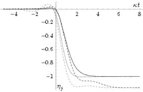
Figure 4: The evolution of the noise sensitivities, $\eta_{j}$, for amplitude errors. The upper curves (solid) correspond to the pulse shapes given in this paper, in Eqs. (10), whilst the lower curves (dotted) are for the pulse shapes presented elsewhere Cirac et al. (1997). The darker traces correspond to the solution for $\eta_{1}(t)$ lighter traces are for $\eta_{2}(t)$.

We have solved the equations numerically (using the numerical differential equation solver provided with Mathematica 4.0) for two different pulse shapes, one given in this paper, Eqs. (10), and the other taken from the proposal for quantum state transfer by Cirac et al. Cirac et al. (1997). The results for the noise sensitivities are plotted in Fig. 4. For each pulse shape the noise sensitivities $\eta_{1}(t)$ and $\eta_{2}(t)$ appear to converge to the same value as $t\rightarrow\infty$, however they do differ by a small but definite amount between pulses shapes, being $-1$ (to the numerical precision of the equation solver) and approximately $-1.17$.

III.4 White Timing Error

Using the same methods, we can consider the effect of timing errors between the pulses applied to the cavities. In this case it makes sense to define only one noise sensitivity, $\eta$, since we may assume that the pulse on the first atom defines the origin of time, and thus it will be errors in the timing of the second pulse relative to the first that will contribute to state transfer errors.

For timing errors, the noisy pulse shape is given by

$$\tilde{g}_{2}(t) = g_{2}(t+\xi(t)),$$ (23)

$$\approx g_{2}(t)+\xi(t)g_{2}^{\prime}(t),$$

where the second line follows by expanding to first order in the quantity $\xi(t)$. It may be seen from this form that $\Delta g_{2}(t)=g_{2}^{\prime}(t)$, and for the pusposes of illustration, we will again take the errors to be $\delta$-correlated, $\langle\xi(t)\xi(t^{\prime})\rangle=\epsilon\delta(t-t^{\prime})$.

The result of the numerical solutions for the corrections to the density matrix are shown in Fig. 5. In this case the pulse shape presented in this paper is very slightly more susceptible to timing errors than the pulse shape given by Cirac et al. Cirac et al. (1997).

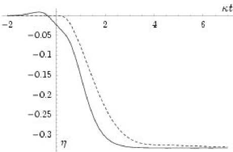
Figure 5: The evolution of the noise sensitivities, $\eta$, for timing errors. The lower curve corresponds to the pulse shapes given in this paper, in Eqs. (10), whilst the upper curve is for the pulse shapes presented elsewhere Cirac et al. (1997).

IV Optimising against noise

From the two examples presented above, we can see that different pulse shapes are more or less sensitive to errors in their generation, depending on the nature of the error. We will now examine how this variation may be used to optimise the pulse shape against sources of error.

The utility of this is in recognising that stochastic noise in control signals contributes to decoherence, which has been noted previously Wellard and Hollenberg (2001). Whilst in that work, the decoherence attributable to stochastic noise was found to be much less than that due to other effects (environment), the calculation was based on a nominally constant control signal with stochastic noise superposed. The situation we consider here, though in a different system, is slightly more general in that the Hamiltonian is explicitly time dependent. Thus the errors in the control pulse will not be simply the intrinsic (e.g. thermal) noise associated with the power source, but also dynamic errors associate with signal generation, e.g. due to digitisation of a nominally continuous pulse, or errors in timing.

IV.1 Optimisation Strategy

In principle, the problem of optimising the pulse shape against noise may be understood in terms of constrained optimisation. We wish to choose a pulse shape that minimises the noise sensitivity, $\eta_{j}(+\infty)$, subject to the constraint that it satisfies the condition of pulse transfer, i.e. $\alpha_{2}(+\infty)=1$. Conceptually, this would provide us with another equation to supplement Eqs. (6) which then makes the number of equations and unknowns equal, thereby specifying the pulse shape uniquely. In practise, we could formulate this problem in terms of Lagrange multipliers Bressoud (1991), and derive the following constrained optimisation equations

$$\frac{\mathcal{D}\eta_{j}(+\infty)}{\mathcal{D}g_{1}(\tau)}+\lambda\frac{\mathcal{D}\alpha_{2}(+\infty)}{\mathcal{D}g_{1}(\tau)} = 0,$$ (24)

$$\alpha_{2}(+\infty)=1,$$ (25)

where the operator ${\mathcal{D}}/{\mathcal{D}g_{1}(\tau)}$ represent the functional derivative with respect to the function $g_{1}(\tau)$, and $\lambda$ is an unknown Lagrange multiplier. We have introduced two more equations, and one more unknown, to bring the total number of each to seven. Since we have chosen $g_{2}(\tau)=g_{1}(-\tau)$ we do not consider functional derivatives with respect to $g_{2}(t)$. Although we don’t prove it formally, we find that $\eta_{1}(+\infty)=\eta_{2}(+\infty)$ in all numerical calulations we have performed, so we only consider variational derivatives with respect to $\eta_{1}(+\infty)$.

In fact, computing either of the above functional derivatives requires the solution of a set of differential equations that are of essentially the same form as Eq. (11a), since they are formulated by taking variational derivatives of the master equation with respect to $g_{1}(\tau)$, which must then be integrated. Since we do not have an analytic solution to the master equations for an arbitrary pulse shape, it is difficult to see how practically to make use of these equations, except for very small scale discretisations.

Another approach is to use numerical substitution. Here, we discretise the pulse shape, defining $g_{j}=g_{1}(t_{j})$ for several discrete times $t_{j}=t_{0},\ldots,t_{n-1}$ (setting $g_{n}=0$), then interpolating between points. We allow all but $g_{0}$ to be variational parameters, and $g_{0}$ is chosen depending on $g_{1},\ldots,g_{n-1}$ to satisfy the constraint, $\alpha_{2}(+\infty)=1$, which is the numerical equivalent of a substitution for $g_{0}$ in terms of all other variational parameters. We then have $n-1$ variational parameters, $g_{1},\ldots,g_{n-1}$, available for unconstrained optimisation of $\eta_{1}(+\infty)$, for which we may use an unconstrained optimisation scheme. In the details of this method, the discretisation points are chosen to be in the domain $t\geq 0$, and $g_{0}$ is determined from $g_{1},\ldots,g_{n-1}$ by use of the method outlined by Cirac et al. Cirac et al. (1997) (and at the end of section II.1 in this paper) which determines the efficacy of a given pulse shape in terms of its form for $t\geq 0$.

IV.2 Numerical Results

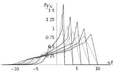
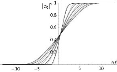
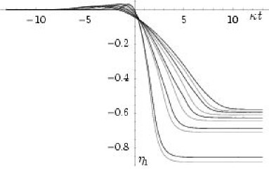
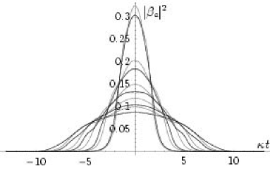
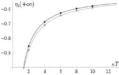
Figure 6: (a) Optimised pulse shapes using three equally spaced points (light), and six equally spaced points (dark) for each of five different pulse widths. (b) Plot of $\alpha_{2}(t)^{2}=\langle e0g0|\rho_{0}(t)|e0g0\rangle$ for each of the pulses. (c) Plot of $\eta_{1}(t)$ showing noise sensitivity for the same pulses. (d) $\beta_{a}(t)^{2}=2\langle g1g0|\rho_{0}(t)|g1g0\rangle$ for each pulse. (e) Showing $\eta_{1}(+\infty)$ versus $T$ (points), and a fit to the data (solid) using a hyperpbolic relation. In all figures, traces from steepest to shallowest correspond to narrowest to broadest pulses in (a), with light traces corresponding to three-point optimisations, and dark traces to six-point optimisations.

A number of numerical optimisations are performed according to the numerical substitution scheme outlined above. In one set of optimisations, three points are allowed vary, and one of them, at $t=0$, is used to satisfy the condition for pulse transfer. The locations of the other two points are equally spaced between $t=0$ and a fourth location, $t=T$, where the function is zero, i.e. the two intermediate points are located at $t=T/3$ and $t=2T/3$. These intermediate points are varied to optimise the pulse shape. The pulse shapes that result from the three-point optimisation process are presented as the lighter traces in Fig. 6 for five different values of $\kappa T=2,4,6,8$ and 10.

In the other set of optimisations, six points are allowed to vary, again with the one at $t=0$ being used to satisfy the condition for successful pulse transfer. The remaining five points are also equally spaced between $t=0$ and $t=T$, for the same values of $T$ as above, and the optimal pulse shapes for the six-point optimisations are shown as the darker traces in Fig. 6.

Figure 6 demonstrates that the various pulses shown in Fig. 6 do each implement quantum state transfer successfully, since $|\alpha_{2}(t)|^{2}\rightarrow 1$ as $t\rightarrow\infty$ for all pulses. The figure also shows that as the width of the pulse becomes broader, proportional to $T$, the transfer process takes longer, so the slope of $|\alpha_{2}(t)|^{2}$ becomes shallower.

Figure 6 shows the noise sensitivity, $\eta_{1}(t)$, for each of the pulses in Fig. 6. Naturally, the value of $\eta_{1}(+\infty)$ gets closer to zero (i.e. better) as the number of optimisation points is increased, and it also gets better as the width of the pulse increases. It may be compared with Fig. 4 which shows the noise sensitivity for the two analytic solutions discussed earlier and the optimisation process has clearly produced pulses that are significantly less sensitive to noise in the laser pulses than either of the analytic solutions discussed earlier in this paper. The best pulse shape computed in the optimisations performed here is that with $T=10$, and has the limit $\eta_{1}\rightarrow-0.58$ as $t\rightarrow\infty$. It appears that the optimisation procedure selects solutions with lower amplitudes, and this occurs because the form of noise we have assumed in this set of examples is proportional to the amplitude of the control pulse, thus lowering the amplitude tends to lower the effect of the noise.

Figure 6 shows that the photon wave-packet transmitted between the cavities, which is proportional to $\beta_{a}(t)$, becomes broader. It may be seen from Eqs. (7) and (8) that $\int_{-\infty}^{+\infty}|\beta_{a}(t)|^{2}dt=1$, and the numerical solutions satisfy this to around one part in $10^{5}$.

Figure 6 plots the limiting value of $\eta_{1}$ versus $T$, the time after which $g_{1}$ is zero, for the three-point (light) and six-point (dark) optimisations. The solid curves are fitted using a function of the form $a+\frac{b}{c+T}$, where $a,b$ and $c$ are fitting parameters. In both cases, the surprisingly close fit has $a=-0.5$ to better than one part in $10^{-3}$, suggesting that the ultimate limit to the optimisation process is an infinitely wide pulse with $\eta_{1}(+\infty)=-0.5$. This indicates that the effect of the noise cannot be removed by allowing the pulse duration to become infinitely long.

V Discussion

The results presented in Fig. 6 above show that there is a clear possibility of selecting pulse shapes that are more or less sensitive to fluctuations therein. Figures 4 and 5 show that pulses which perform better with respect to one source of error may perform worse with respect to another, so in a realistic implementation of the optimisations presented here, detailed knowledge of the sources of stochastic error in the pulses would be required.

The reduction in transfer error from an optimised pulse is moderate in the case of white amplitude noise considered here, reducing the error in the transfer by a factor of a little over two compared to the original pulse shape presented by Cirac et al. Cirac et al. (1997). Though this is not a very large improvement, regardless of the shape chosen, pulse shaping will be needed to implement quantum state transfer, and so it is prudent to select the pulse with lowest noise sensitivity.

The order of magnitude of transfer errors produced by the pulse are set by the magnitude of $\epsilon_{j}$, which is essentially the relative variance of the pulse fluctuations, integrated over time. As mentioned earlier, for white amplitude noise, one candidate that could produce this is intrinsic amplitude fluctuations in the laser. For a cw laser, this can almost immediately be ruled out as a legitimate error source, since the relative RMS amplitude lasers in e.g. a diode laser are of order $10^{-6}$ Ohtsu (1992), so the variance is $\epsilon_{j}\sim 10^{-12}$, which is completely negligible.

A more likely source of error may be due to either the pulse generator or the pulse shaper. Whilst the original proposal for quantum state transfer was based on atomic states, we have had in mind the application of this scheme to electron spin states confined to quantum dots, with the dots contained within a linear microcavity, in a similar scheme to that illustrated by Benson et al. Benson et al. (2000) and suggested by Imamoḡlu et al. Imamoḡlu et al. (1999); Imamoḡlu (2000). For a cavity of length 1 $\mu$m, the free spectral range is around $10^{14}$ Hz, and if we imagine one of the Bragg mirrors has transmissivity of $10^{-3}$, then the cavity loss rate is around $\kappa\approx 10^{11}\mathrm{sec}^{-1}$. This is an optimistic but not unreasonable estimate for the transmissivity, e.g. Lidzey et al. Lidzey et al. (1998) report a microcavity $Q$-factor of 125 (based on a cavity linewidth of $\sim 20$ meV and a mode frequency of 2.88 eV) for a $\lambda/2$ cavity, which corresponds to a mirror transmissivity of $T_{\mathrm{mir}}=0.025$ Mandel and Wolf (1995), and good quality cavity linewidths may be as low as 0.5 meV Yamamoto and Imamoḡlu (1999), corresponding to $T_{\mathrm{mir}}=5\times 10^{-4}$.

Since $1/\kappa$ sets the time scale of the control pulse (see e.g. Fig. 6), the typical width of the pulse is $\sim 10$ ps. Weiner Weiner (2000) gives a relation for the shortest temporal feature that one may generate as $\delta t=T/\eta$ where $T$ is the largest temporal window, and $\eta$ is a measure of the potential complexity of the pulse. Typical values are quoted as $T=26.4$ ps, which is the same order of magnitude as $1/\kappa$, and $\eta=264$, so $\delta t\approx 10^{-13}$ s. Thus, if we assert that fluctuations at time scales less than $\delta t$ are uncontrolled, then an upper estimate on relative amplitude fluctuations might be $\delta g\approx g^{\prime}(t)\delta t$, which means that uncontrolled relative amplitude fluctuations from the pulse shaper could be as large as $1/\eta\sim 0.01$, which is certainly not negligible.

We note in passing that the time scale of 10 ps is roughly coincident with the characteristic time required for an electron in a travelling quantum dot generated by a surface acoustic wave (SAW) (velocity $\approx 3000$ m s^-1), to traverese a distance of 1 $\mu$m, which is the typical dimension of a SAW wavelength Barnes et al. (2000), as well as a typical minimum spot size for an optical CW laser at its focal point. Therefore, if a microcavity were constructed at the end of the SAW based quantum computer proposed in Barnes et al. (2000), then a CW laser focused at the center of the microcavity with a cross-sectional intensity profile shaped such that an electron passing through the microcavity experiences a time varying electric field which implements quantum state transfer (e.g Eq. (10c)), then the quantum state transfer scheme discussed in this paper could be used for both an interconnect between several SAW quantum processors and for electron-spin measurement (detection of a photon out of the cavity corresponds to a definite spin state of the electron).

This paper has been fundamentally concerned with time dependent Hamiltonians, which are, conceptually, generally applicable to schemes for implementation of quantum computation. We therefore suppose that in many quantum gates implemented with time dependent control pulses, there could be some advantage in shaping the control pulses to be minimally sensitive to errors, so the ideas discussed in this paper may well be generalisable to other quantum information applications.

VI Summary

We have analyzed the effect of stochastic noise on a control pulse that implements quantum state transfer between two atoms or quantum dots. We have found an alternate analytic solution for laser pulses that implement quantum state transfer, and using the two analytic solutions we have available, we found that although different control pulses are capable of implementing quantum state transfer, they may have different sensitivities to noise, depending both on their shape and the source of the noise. We then provided a method for calculating pulse shapes with lower noise sensitivities thereby optimising the pulse shape. This method was demonstrated to produce more optimal control pulses for the case of noise that is proportional to the control pulse amplitude with a white spectrum. A number of successively better pulse shapes were presented, and extrapolating the improvement in the noise sensitivity to its limit (i.e. for infinitely wide pulses) strongly suggests that the influence of this particular form of noise cannot be cancelled completely.