Self-induced transparency and giant nonlinearity in doped photonic crystals

Abstract

Photonic crystals doped with resonant atoms allow for uniquely advantageous nonlinear modes of optical propagation: (a) Self-induced transparency (SIT) solitons and multi-dimensional localized ”bullets” propagating at photonic band gap frequencies. These modes can exist even at ultraweak intensities (few photons) and therefore differ substantially either from solitons in Kerr-nonlinear photonic crystals or from SIT solitons in uniform media. (b) Cross-coupling between pulses exhibiting electromagnetically induced transparency (EIT) and SIT gap solitons. We show that extremely strong correlations (giant cross-phase modulation) can be formed between the two pulses. These features may find applications in high-fidelity classical and quantum optical communications.

I Introduction

Photonic crystals (PCs) can exhibit an interplay between Bragg reflections, which block the propagation of light in photonic band gaps (PBGs) pbg-bib ; yablon ; john ; joannopoulos ; defect_a ; defect_b , and the dynamical modifications of these reflections by nonlinear light-matter interactions kofman ; john_wang ; pl ; Ze95 ; Scal94 ; Scal94a . A very interesting situation arises when foreign atoms or ions—dopants—with transition frequencies within the PBG are implanted in the PC kofman ; john_wang ; pl . Then light near one of these frequencies resonantly interacts with the dopants and is concurrently affected by the PBG dispersion. Consequently, highly nonlinear processes with a rich variety of unusual PC-related features are anticipated.

Our aim in recent years has been to identify those regimes of nonlinear optical propagation in doped PCs that allow transmission of extremely weak pulses, while filtering out undesirable noise, and are therefore highly advantageous for optical communications, data storage and processing, near or at the quantum limit. These requirements are satisfied by novel regimes surveyed in this paper that have been theoretically discovered and investigated by us: a) Self-induced transparency (SIT) solitons propagating inside or near a PBG at a frequency that is near resonant with the transition frequency of the dopant Kuri2001 ; Kozh95 ; Kozh98a ; Opat99 . This peculiar form of gap solitons (GSs) is immune to resonant absorption even for a small number of photons, and may also possess two- or three-dimensional (2D or 3D) localization in the form of light bullets (LBs)Blaa00a (Sec. II). b) Cross-coupling of SIT and electromagnetically-induced transparency (EIT) pulses in PCs. We put forward a new regime in Sec. III: a strong modulation of the phase of a weak pulse subject to EIT by a control pulse in the form of an SIT GS moving at the same slow velocity. Thereby giant cross-phase modulation can be formed between the GS and the EIT pulses. In Sec. IV we summarize and discuss our findings in this paper.

II Self-induced transparency (SIT) gap solitons

II.1 Background

A GS is usually understood as a self-localized moving or standing (quiescent) bright region, where light is confined by Bragg reflections against a dark background. The soliton spectrum is tuned away from the Bragg resonance by the nonlinearity at sufficiently high field intensities. The first type of GS had been predicted Chri89 ; Acev89 ; Feng93 ; Ster94 , and later observed Eggl96 , in a Bragg grating possessing Kerr-nonlinearity. A principally different mechanism of GS formation has been theoretically discovered by our group in a periodic array of thin layers of resonant two-level atoms (TLA) separated by half-wavelength nonabsorbing dielectric layers, i.e., a resonantly absorbing Bragg reflector (RABR) Kuri2001 ; Kozh95 ; Kozh98a ; Opat99 . As opposed to the $2\pi$-solitons arising in SIT, i.e., resonant field–TLA interaction in uniform media McCa67 ; McCa69 , their GS counterparts in a RABR may have an arbitrary pulse area Kozh95 ; Kozh98a . It must be stressed that stable, moving or standing, GS solutions have been consistently obtained only in a RABR with thin active TLA layers. By contrast, the case of a periodic structure uniformly doped with active TLA calls either for a solution of the wave (Maxwell) equation without the spatial slowly-varying envelope approximation (SVEA), or for a solution of an infinite set of coupled Bloch equations for all spatial harmonics of the atomic polarization (Fourier components) Kuri2001 . Therefore, an attempt Akoz98 to obtain a self-consistent solution for a uniformly-doped periodic structure by imposing the SVEA, or by arbitrarily truncating the infinite hierarchy of equations for the harmonics of atomic population inversion and polarization to its first two orders, is generally unjustified. In fact, it can be shown numerically to fail for many parameter values.

In the simplest case of a uniform (bulk) medium, when the driving field is resonant with the atomic transition, the TLA Bloch equations can be easily integrated and the Maxwell equation then reduces to the sine-Gordon equation

$$\frac{\partial^{2}\theta}{\partial\zeta\partial\tilde{\tau}}=-\sin{\theta}$$ (1)

for the pulse area $\theta=\int_{-\infty}^{t}\Omega\,dt^{\prime}$, i.e., the time integral of the Rabi frequency $\Omega$. Equation (1) is written in terms of the dimensionless variables $\tilde{\tau}=(t-n_{0}z/c)/\tau_{0}$ and $\zeta=n_{0}z/c\tau_{0}$, where $\tau_{0}=\frac{n_{0}}{\mu}\sqrt{\frac{\hbar}{2\pi\omega_{c}\varrho_{0}}}$, is the cooperative resonant absorption time, $\varrho_{0}$ being the TLA density (averaged over $z$), $\mu$ the dipole moment of the TLA transition at frequency $\omega_{0}$ and $n_{0}$ is the refraction index of the host medium. This sine-Gordon equation is known to have solitary-wave solutions, which propagate without attenuation or distortion with a conserved pulse area of $2\pi$ McCa67 ; McCa69 . These SIT solitons have the form:

$${\Omega}(\zeta,\tilde{\tau})=(\tau_{0})^{-1}A_{0}\text{sech}[\beta(\zeta-v\tilde{\tau})],$$ (2)

where the pulse width $\beta$ is an arbitrary real parameter uniquely defining the amplitude $A_{0}=2/\beta$ and group velocity $v=1/\beta^{2}$ of the soliton. In what follows, Eq. (2) will be compared with an SIT GS in a RABR.

II.2 SIT in RABR: The Model

Let us assume Kuri2001 ; Kozh95 ; Kozh98a ; Opat99 a one-dimensional (1D) periodic modulation of the linear refractive index $n^{2}(z)=n_{0}^{2}[1+a_{1}\cos(2k_{c}z)]$. The periodic grating gives rise to a PBG with a central frequency $\omega_{c}=k_{c}c/n_{0}$ and gap edges at $\omega_{1,2}=\omega_{c}\left(1\pm a_{1}/4\right)$. The electric field $E$ of a pulse propagating along $z$ can be expressed by means of the dimensionless quantities $\Sigma_{\pm}\equiv 2\tau_{o}\mu\hbar^{-1}({\cal E}_{F}\pm{\cal E}_{B})$, where ${\cal E}_{F}$ and ${\cal E}_{B}$ denote the slowly varying amplitudes of the forward and backward propagating fields, respectively, as

$$E(z,t)=\hbar(\mu\tau_{0})^{-1}\left\{{\rm Re}[\Sigma_{+}(z,t)e^{-i\omega_{c}t}]\cos k_{c}z-{\rm Im}[\Sigma_{-}(z,t)e^{-i\omega_{c}t}]\sin k_{c}z\right\}.$$ (3)

We further assume that very thin TLA layers (much thinner than $1/k_{c}$), whose resonance frequency $\omega_{0}$ is close to the gap center $\omega_{c}$, are placed at the maxima of the modulated refraction index (Fig. 1). They are located at positions $z_{j}$ such that

$$e^{ik_{c}z_{2j}}=1,\qquad e^{ik_{c}z_{2j+1}}=-1,$$ (4)

i.e., the TLA density is described by $\varrho=\varrho_{0}\lambda/2\sum_{j}\delta(z-z_{j})$, where $\lambda=2\pi/k_{c}$ is the wavelength.

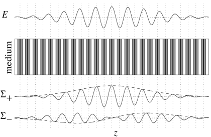
Figure 1: Schematic description of the periodic RABR and of the decomposition of the electric field $E$ into modes $\Sigma_{+}$ and $\Sigma_{-}$. The shading represents regions with different index of refraction; the darker the shading the larger $n$ is. The black regions correspond to the TLA layers. The localization of the field envelope over $\sim 20$ structure periods is shown for the sake of visualization; in reality, the field is localized over a hundred or more periods.

The Bloch equations for the slowly varying polarization envelope $P$ and inversion $w$ in the even numbered layers can be obtained (in the slowly varying envelope approximation) by substituting for the Rabi frequency $\Omega=\tau_{0}^{-1}(\Sigma_{+}\cos k_{c}z+i\Sigma_{-}\sin k_{c}z)$ and applying Eq. (4) at the positions of these layers:

$$\frac{\partial P}{\partial\tau} = -i\delta P+\Sigma_{+}w,$$ (5)

$$\frac{\partial w}{\partial\tau} = -{\rm Re}\ \left(\Sigma_{+}P^{*}\right).$$ (6)

Combining Eqs. (5) and (6), one can eliminate the TLA population inversion: $w=\sqrt{1-|P|^{2}}$. The remaining equation, together with the Maxwell equations for $\Sigma_{\pm}$ (driven by $P$), form a closed system,

$$\frac{\partial^{2}\Sigma_{+}}{\partial\tau^{2}}-\frac{\partial^{2}\Sigma_{+}}{\partial\zeta^{2}} = \eta^{2}\Sigma_{+}+2i(\eta-\delta)P-2\sqrt{1-|P|^{2}}\Sigma_{+},$$ (7)

$$\frac{\partial^{2}\Sigma_{-}}{\partial\tau^{2}}-\frac{\partial^{2}\Sigma_{-}}{\partial\zeta^{2}} = -\eta^{2}\Sigma_{-}-2\frac{\partial P}{\partial\zeta},$$ (8)

$$\frac{\partial P}{\partial\tau} = -i\delta P-\sqrt{1-|P|^{2}}\Sigma_{+},$$ (9)

where $\tau\equiv t/\tau_{0}$, $\zeta\equiv\left(n_{0}/c\tau_{0}\right)z$ and $\delta\equiv(\omega_{0}-\omega_{c})\tau_{0}$ are the dimensionless time, coordinate, and detuning, respectively, and $\eta=l_{\rm abs}/l_{\rm refl}=a_{1}\omega_{c}\tau_{0}/4$ is the dimensionless modulation strength, which can be expressed as the ratio of the TLA absorption distance $l_{\rm abs}=\tau_{0}c/n_{0}$ to the Bragg reflection distance $l_{\rm refl}=4c/(a_{1}\omega_{c}n_{0})$. We emphasize that the above equations are obtained using the SVEA, which is valid under the assumption that the Bragg reflection does not appreciably change the pulse envelope over a distance of a wavelength, $l_{\rm refl}\gg\lambda$, whence $a_{1}\ll 2/\pi$.

To reach general understanding of the dynamics of the model, one should first consider the spectrum produced by the linearized version of Eqs. (7)–(9), which describes weak fields in the limit of infinitely thin TLA layers. Setting $\Sigma_{+}=Ae^{i(\kappa\zeta-\chi\tau)}$, $\Sigma_{-}=Be^{i(\kappa\zeta-\chi\tau)}$, $w=-1$, and $P=Ce^{i(\kappa\zeta-\chi\tau)}$, we obtain from the linearized equation (9) that $C=i(\delta-\chi)^{-1}A$. Substituting this into Eqs. (7) and (8), we arrive at the dispersion relation for the wavenumber $\kappa$ and frequency $\chi$ in the form

$$(\chi^{2}-\kappa^{2}-\eta^{2})(\chi-\delta)\times\left\{(\chi-\delta)\left[\chi^{2}-\kappa^{2}-(2+\eta^{2})\right]+2(\eta-\delta)\right\}=0.$$ (10)

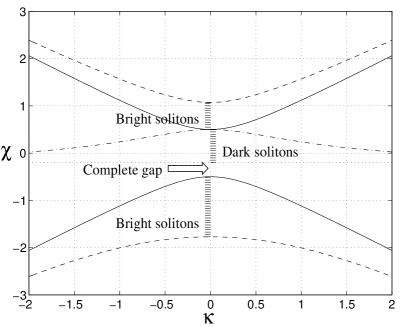
Figure 2: The RABR dispersion curves at $\eta=0.5$ and $\delta=-0.2$. The solid lines show the dispersion branches corresponding to the ‘bare’ (noninteracting) grating, while the dashed and dash-dotted lines stand for the dispersion branches of the grating ‘dressed’ by the active medium. The frequency bands that support the standing dark and bright solitons are shaded.

Different branches of the dispersion relation generated by Eq. (10) are shown in Fig. 2. The roots $\chi=\pm\sqrt{\kappa^{2}+\eta^{2}}$ (corresponding to the solid lines in Fig. 2) originate from the driven equation (8) and represent the dispersion relation of a Bragg reflector with the gap $|\chi|<\eta$, that does not feel the interaction with the active layers. Important roots of Eq. (10) are those of the expression in the curly brackets, shown by the dashed and dash-dotted lines in Fig. 1. These roots correspond to nontrivial spectral features: bright or dark solitons in the indicated (shaded) bands.

The frequencies corresponding to $k=0$ are $\chi_{0}=\eta$ and $\chi_{0,\pm}=-(\eta-\delta)/2\pm\sqrt{2+(\eta+\delta)^{2}/2}$, while at $k^{2}\to\infty$ the asymptotic expressions for different branches of the dispersion relation are $\chi=\pm k$ and $\chi=\delta+2\left(\eta-\delta\right)k^{-2}$. Thus, the linearized spectrum always splits into two gaps, separated by an allowed band, except for the special case, $\eta=\eta_{0}\equiv\delta/2+\sqrt{1+\delta^{2}/4}$, when the upper gap closes down. The upper and lower band edges are those of the periodic structure, shifted by the induced TLA polarization in the limit of a strong reflection. They approach the SIT spectral gap for forward- and backward-propagating waves Mant95 in the limit of weak reflection. The allowed middle band corresponds to a polaritonic excitation (collective atomic polarization) in the periodic structure.

II.3 Standing (quiescent) self-localized pulses

We seek the stationary solutions of Eqs. (7) and (9) corresponding to bright solitons in the form

$$\Sigma_{+}=e^{-i\chi\tau}{\cal S}(\zeta),\qquad P=i\ e^{-i\chi\tau}{\cal P}(\zeta)$$ (11)

with real ${\cal P}$ and ${\cal S}$. Substituting this into (9), we eliminate ${\cal P}$ in favor of ${\cal S}$ and obtain an equation for ${\cal S}(\zeta)$,

$$\frac{d^{2}{\cal S}}{d\zeta^{2}}=(\eta^{2}-\chi^{2}){\cal S}-2{\cal S}\frac{(\eta-\chi)\cdot{\rm sign}(\chi-\delta)}{\sqrt{(\chi-\delta)^{2}+{\cal S}^{2}}}.$$ (12)

It then follows Kozh98a that bright solitons can appear in two frequency bands $\chi$, the lower band being $\chi_{1}<\chi<{\rm min}\{\chi_{2},-\eta,\delta\}$, and the upper band being ${\rm max}\{\chi_{1},\eta,\delta\}<\chi<\chi_{2}$, where $\chi_{1,2}\equiv 1/2[\delta-\eta\mp\sqrt{(\eta+\delta)^{2}+8}]$ are the boundary frequencies. The lower band exists for all values $\eta>0$ and $\delta$, while the upper one only exists for the weak-reflectivity case $\delta>\eta-1/\eta$. On comparing these expressions with the spectrum shown in Fig. 2, we conclude that part of the lower gap is always empty from solitons, while the upper gap is completely filled with stationary solitons in the weak-reflectivity case, and completely empty in the opposite limit.

In an implicit form, the solution of Eq. (12) reads

$${\cal S}(\zeta)=2|\chi-\delta|{\cal R}(\zeta)\left(1-{\cal R}^{2}(\zeta)\right)^{-1},$$ (13)

with

$$|\zeta|=\sqrt{2\left|\frac{\chi-\delta}{\chi-\eta}\right|}\left[(1-{\cal R}_{0}^{2})^{-1/2}\tan^{-1}\sqrt{\frac{{\cal R}_{0}^{2}-{\cal R}^{2}}{1-{\cal R}_{0}^{2}}}+(2{\cal R}_{0})^{-1}\ln\left(\frac{{\cal R}_{0}+\sqrt{{\cal R}_{0}^{2}-{\cal R}^{2}}}{{\cal R}}\right)\right],$$ (14)

and ${\cal R}_{0}^{2}=1-|(\chi+\eta)(\chi-\delta)|/2$. This zero-velocity (ZV) gap soliton is always single-humped and its amplitude, found from Eq. (14), is given by

$${\cal S}_{\max}=4{\cal R}_{0}/\sqrt{\left|\chi+\eta\right|}.$$ (15)

To calculate the electric field in the antisymmetric $\Sigma_{-}$ mode, we substitute $\Sigma_{-}=ie^{-i\chi\theta}{\cal A}(\zeta)$ into Eq. (8) and obtain

$${\cal A}^{\prime\prime}+\left(\chi^{2}-\eta^{2}\right){\cal A}=2{\cal P}^{\prime},$$ (16)

which can be easily solved by the Fourier transform, once ${\cal P}(\zeta)$ is known. We note that, depending on the parameters $\eta$, $\delta$ and $\chi$, the main part of the soliton energy can be carried either by the $\Sigma_{+}$ or the $\Sigma_{-}$ mode.

The most drastic difference of these new solitons from the well-known SIT solitons in Eq. (2) is that the area of the ZV soliton (integrated over $\zeta$) is not restricted to $2\pi$, but, instead, may take an arbitrary value. This basic new feature shows that the Bragg reflector can enhance (by multiple reflections) the field coupling to the TLA, so as to make the pulse area effectively equivalent to $2\pi$. In the limit of the small-amplitude and small-area solitons, ${\cal R}_{0}^{2}\ll 1$, Eq. (14) can be easily inverted, the ZV soliton becoming a broad sech-like pulse:

$${\cal S}\approx 2|\chi-\delta|{\cal R}_{0}\,{\rm sech}\left(\sqrt{2\left|\frac{\chi-\eta}{\chi-\delta}\right|}{\cal R}_{0}\zeta\right).$$ (17)

In the opposite limit, $1-{\cal R}_{0}^{2}\rightarrow 0$, i.e., for vanishingly small $|\chi+\eta|$, the the soliton is characterized by a broad central part with a width $\sim\left(1-{\cal R}_{0}^{2}\right)^{-1/2}$ and its amplitude (15) becomes very large. Thus, although the ZV soliton has a single hump, its shape is, in general, strongly different from that of the traditional nonlinear-Schrödinger (NLS) sech pulse.

II.4 Moving solitons

One could expect a translational invariance of the ZV solitons (13) on physical grounds. Hence, a full family of soliton solutions should have velocity as one of its parameters. This can be explicitly demonstrated in the limit of the small-amplitude large-width solitons [cf. Eq. (17)]. We search for the corresponding solutions in the form $\Sigma_{+}(\zeta,\tau)={\cal S}(\zeta,\tau)\exp(-i\chi_{0}\tau)$, $P(\zeta,\tau)=i{\cal P}(\zeta,\tau)\exp(-i\chi_{0}\tau)$ [cf. Eqs. (11)], where $\chi_{0}$ is the frequency corresponding to $k=0$ on any of the three branches of the dispersion relation (10) (see Fig. 2), and the functions ${\cal S}(\zeta,\tau)$ and ${\cal P}(\zeta,\tau)$ are assumed to be slowly varying in comparison with $\exp(-i\chi_{0}\tau)$. Under these assumptions, we arrive at the following asymptotic equation for ${\cal S}(\zeta,\tau)$:

$$\left[2i\frac{\chi_{0}(\chi_{0}-\delta)^{2}-\eta+\delta}{(\chi_{0}-\delta)^{2}}\frac{\partial}{\partial\tau}+\frac{\partial^{2}}{\partial\zeta^{2}}+\frac{\chi_{0}-\eta}{(\chi_{0}-\delta)^{3}}|{\cal S}|^{2}\right]{\cal S}=\left(\eta^{2}-\chi_{0}^{2}+2\frac{\chi_{0}-\eta}{\chi_{0}-\delta}\right){\cal S}.$$ (18)

Since this equation is of the NLS form, it has the full two-parameter family of soliton solutions, including the moving ones Newe92 .

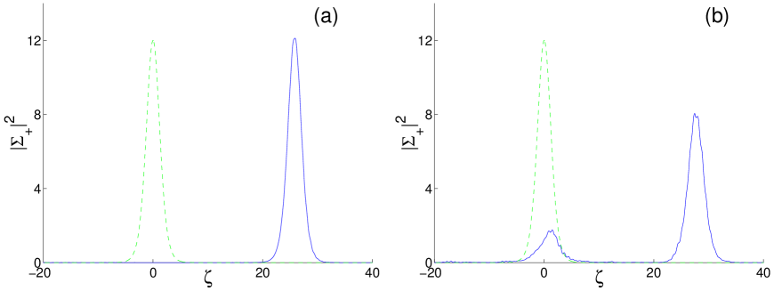
Figure 3: Pulses obtained as a result of ‘pushing’ a zero-velocity RABR soliton (dashed lines): (a) push, characterized by the initial multiplier $\exp(-ip\zeta)$ after a sufficiently long evolution ($\tau=400$) (solid lines). $\delta=0$, $\eta=4$, $\chi=-4.4$, and $p=0.1$. (b) idem, but for $p=0.5$.

In order to check the existence and stability of the moving solitons numerically, the following procedure has been used Kozh98a : Eqs. (7) and (9) were simulated for an initial configuration in the form of the ZV soliton multiplied by $\exp(ip\zeta)$ with some wavenumber $p$, in order to ‘push’ the soliton. The results demonstrate that, at sufficiently small $p$, the ‘push’ indeed produces a moving stable soliton [Fig. 3(a)]. However, if $p$ is large enough, the multiplication by $\exp(ip\zeta)$ turns out to be a more violent perturbation, splitting the initial pulse into two solitons, one quiescent and one moving [Fig. 3(b)].

II.5 Light bullets (spatiotemporal solitons) in PCs

The advantageous properties of SIT GS can be supplemented by immunity to transverse diffraction, i.e., simultaneous transverse and longitudinal self-localization of light in a PC: multi-dimensional spatio-temporal solitons or “light bullets” (LBs) Silb90 have been analytically and numerically predicted by our group to exist and be stable, not only in uniform 2D and 3D SIT media Blaa00 , but also in 2D or 3D periodic structures, wherein SIT solutions combining LB and GS properties are demonstrated Blaa00a . Our objective is to consider the propagation of an electromagnetic wave with a frequency close to $\omega_{c}$ through a 2D PC doped by thin TLA layers. The forward- and backward-propagating components satisfy equations that are a straightforward generalization of the 1D equations (7) and (8)

$$-i\frac{\partial^{3}\Sigma_{+}}{\partial\tau x^{2}}+i\frac{\partial^{3}\Sigma_{-}}{\partial\zeta x^{2}}+\frac{\partial^{2}\Sigma_{+}}{\partial\tau^{2}}-\frac{\partial^{2}\Sigma_{+}}{\partial\zeta^{2}}+\eta\frac{\partial^{2}\Sigma_{+}}{\partial x^{2}}+\eta^{2}\Sigma_{+}-2\frac{\partial P}{\partial\tau}-2i\eta{P}=0,$$ (19)

$$-i\frac{\partial^{3}\Sigma_{-}}{\partial\tau x^{2}}+i\frac{\partial^{3}\Sigma_{+}}{\partial\zeta x^{2}}+\frac{\partial^{2}\Sigma_{-}}{\partial\tau^{2}}-\frac{\partial^{2}\Sigma_{-}}{\partial\zeta^{2}}-\eta\frac{\partial^{2}\Sigma_{-}}{\partial x^{2}}+\eta^{2}\Sigma_{-}+2\frac{\partial P}{\partial\zeta}=0,$$ (20)

where the Fresnel number $F>0$, which governs the transverse diffraction in the 2D and 3D propagation, was incorporated into $x$ denoting the transverse coordinate. The equations for the polarization $P$ and inversion $w$ are the same as Eqs. (5) and (6).

We search for analytical LB solutions of Eqs. (19), (20), (5) and (6), by the following ansatz that reduces in 1D to the exact moving GS Kuri2001 ; Kozh95

$$\Sigma_{+} = A_{0}\sqrt{\text{sech}\Theta_{1}\text{sech}\Theta_{2}}e^{i(\kappa\zeta-\chi\tau)+i\pi/4},$$ (21)

$$\Sigma_{-} = \Sigma_{+}/v,$$ (22)

$$P = \sqrt{\text{sech}\Theta_{1}\text{sech}\Theta_{2}}\{(\tanh\Theta_{1}+\tanh\Theta_{2})^{2}+$$ (23)

$${}\frac{\delta-\eta}{4\eta}C^{4}\bigl{[}(\tanh\Theta_{1}-\tanh\Theta_{2})^{2}-2(\text{sech}^{2}\Theta_{1}+\text{sech}^{2}\Theta_{2})\bigr{]}^{2}\}^{1/2}e^{i(\kappa\zeta-\chi\tau)+i\nu},$$

$$w = \left[1-|{P}|^{2}\right]^{1/2},$$ (24)

with $\Theta_{1}(\tau,\zeta)\equiv\beta(\zeta-v\tau)+\Theta_{0}+Cx$, $\Theta_{2}(\tau,\zeta)\equiv\beta(\zeta-v\tau)+\Theta_{0}-Cx$, the phase $\nu$ and coefficients $\Theta_{0}$ and $C$ being real constants, while the other parameters are defined as $A_{0}=2\sqrt{\delta/\eta-1}$, $\beta=\sqrt{\delta/\eta+1}$, $v=-\sqrt{(\delta-\eta)/(\delta+\eta)}$, $\kappa=-\sqrt{\delta^{2}-\eta^{2}}$, and $\chi=\delta$.

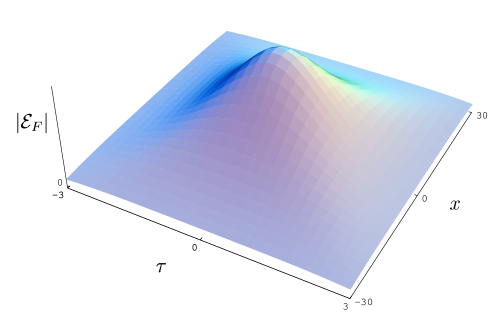
Figure 4: The forward-propagating electric field of the two-dimensional ‘light bullet’ in the Bragg reflector, $|{\cal E}_{F}|$, vs. time $\tau$ and transverse coordinate $x$, after having propagated the distance $z=1000$. The parameters are $\eta=0.1$, $\delta=0.2$, $C=0.1$ and $\Theta_{0}=-1000$. The field is scaled by the constant $\hbar/4\tau_{0}\mu n_{0}$.

The ansatz (21)- (24) satisfies Eqs. (19) and (20) exactly, while Eqs. (5) and (6) are satisfied to order $\sqrt{\delta/\eta-1}C^{2}$, which requires that $\sqrt{\delta/\eta-1}C^{2}\ll 1$. The ansatz applies for arbitrary $\eta$, admitting both weak ($\eta\ll 1$) and strong ($\eta>1$) reflectivities of the Bragg grating, provided that the detuning remains small with respect to the gap frequency. Comparison with numerical simulations of Eqs. (19), (20), (5) and (6), using Eqs. (21)-(24) as an initial configuration, tests this analytical approximation and shows that it is indeed fairly close to a numerically exact solution; in particular, the shape of the bullet remains within 98% of its originally presumed shape after having propagated a large distance, as is shown in Fig. 4.

Three-dimensional (3D) LB solutions with axial symmetry have also been constructed in an approximate analytical form and successfully tested in direct simulations, following a similar approach Blaa00a . Generally, they are not drastically different from their 2D counterparts described above.

II.6 Information transmission by SIT GSs and LBs

The efficiency of information transmission is characterized either by channel (information) capacity $C=W\ln(I_{s}/I_{n})$, where $W$ is the bandwidth and $I_{s}/I_{n}$ is the ratio of the signal-to-noise intensities, or by the data transmission density $D=NM$, where $N$ is the number of bits per channel and $M$ is the number of accessible channels. Both $C$ and $D$ can be very high in the case of a SIT GS or LB for the following reasons: (a) The bandwidth $W$ is large, being limited by the PBG width, which can be very large in the optical domain. At the same time, noise is very effectively suppressed by the Bragg reflection and by the absence of diffraction losses in the case of a LB. (b) The maximal transmission density $D$ can be estimated Mossberg as the ratio of the accessible bandwidth, in our case the PBG width (in excess of $10^{13}$ s^-1 in the optical domain), to the spontaneous linewidth ($10^{6}$ s^-1 for rare-earth ions). Hence, these modes of transmission can be very effective for optical communications.

III Cross coupling between electromagnetically-induced and self-induced transparency pulses

III.1 EIT in bulk media: Background

Electromagnetically induced transparency (EIT) is based on the phenomenon of coherent population trapping eit_a ; eit_b , in which the application of two laser fields to a three-level atomic system creates the so-called “dark state”, which is stable against absorption of both fields. Consider a four-level atomic system whose level configuration is depicted in Fig. 5(a). The phase shift and absorption of an optical field $E_{i}$ are given by the real and imaginary parts of its complex polarizability $\alpha_{i}$. In the absence of the “control” field $E_{b}$, the usual EIT spectrum [Fig. 5(b)] for the weak probe field $E_{a}$ exhibits vanishing phase shift and absorption [$\text{Re}(\alpha_{a})=\text{Im}(\alpha_{a})=0$] at the two-photon Raman resonance $\omega_{a}=\omega_{21}+\omega_{d}$, where $\omega_{a}$ and $\omega_{d}$ are the frequencies of the probe and driving fields, respectively, and $\omega_{ij}$ is the frequency of the atomic transition $\,|i\rangle\to\,|j\rangle$. An off-resonant control field $E_{b}$ with the frequency $\omega_{b}$ such that $|\Delta_{b}|=|\omega_{b}-\omega_{43}|\gg\gamma_{4}$, where $\gamma_{i}$ is the decay rate of the corresponding atomic level, induces an ac Stark shift of level $\,|3\rangle$ and thereby shifts the EIT spectrum [Fig. 5(b)].

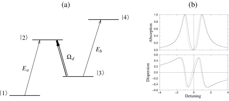
Figure 5: (a) Schematic representation of the atomic system interaction with strong driving field on the transition $\,|2\rangle\to\,|3\rangle$ and weak fields $E_{a}$ and $E_{b}$ on the transitions $\,|1\rangle\to\,|2\rangle$ and $\,|3\rangle\to\,|4\rangle$, respectively. (b) Absorption and dispersion spectra of the $E_{a}$ field in the absence (solid line) or presence (dashed line) of the $E_{b}$ field.

Due to the steepness of the dispersion curve in the vicinity of the Raman resonance, $|\partial_{\omega_{a}}\text{Re}(\alpha_{a})|\gg|\partial_{\omega_{a}}\text{Im}(\alpha_{b})|$, this Stark shift leads to a large phase shift along with small absorption of the probe field $E_{a}$:

$$\phi_{a}=\text{Re}(\alpha_{a})z\simeq-\frac{\alpha_{0}\gamma_{2}|\Omega_{b}|^{2}}{2\Delta_{b}|\Omega_{d}|^{2}}z,\;\;\;\text{Im}(\alpha_{a})=-\frac{\gamma_{4}\text{Re}(\alpha_{a})}{2\Delta_{b}}\ll\text{Re}(\alpha_{a}),$$ (25)

where $\alpha_{0}$ is the resonant absorption coefficient of the medium at the frequency $\omega_{21}$ and $\Omega_{i}=\mu_{ij}E_{i}/\hbar$ is the Rabi frequency of the corresponding field ($\mu_{ij}$ the dipole matrix element on the respective transition). This is the essence of the so-called giant Kerr cross-phase modulation of a probe field by a control field, introduced first by Schmidt and Imamoğlu imam . Later Harris and Yamamoto harris_a have predicted that a resonant control field $E_{b}$ with $|\Delta_{b}|<\gamma_{4}$ can destroy the coherence between the two ground levels $\,|1\rangle$ and $\,|3\rangle$, which leads to a two-photon absorption $\text{Im}(\alpha_{a,b})=\frac{\alpha_{0}\gamma_{2}|\Omega_{b,a}|^{2}}{\gamma_{4}|\Omega_{d}|^{2}}$, that is, the medium absorbs two fields simultaneously, but does not absorb one field alone. This is the essence of a probe-photon switch, conditional on the presence of control photons.

The main limitation of the above schemes imam ; harris_a ; harris_b stems for the fact that the effective interaction length is limited by the mismatch between the group velocity of the slowly propagating $E_{a}$ field, $v^{(a)}_{g}\simeq\frac{2|\Omega_{d}|^{2}}{\alpha_{0}\gamma_{3}}\ll c/n_{0}$ and that of the nearly-free propagating $E_{b}$ field, $v^{(b)}_{g}\simeq c/n_{0}$. For weak (few-photon) pulses, this mismatch ultimately limits the maximal phase shift or absorption of the probe in the presence of the control field.

III.2 Simultaneous EIT and SIT in RABR

In this section we propose a new implementation of the cross-phase modulation, in which the group velocities of both fields can be matched, allowing one to obtain any desired phase shift of the probe field with a weak control field. To this end, we consider the same configuration as in Sec. II, leading to SIT GS and LB solutions: a PC periodically doped by thin layers of atoms at the maxima of its refractive index. However, the multi-level structure of the atoms is now playing a role: it is shown in Fig. 6, along with the polarizations and propagation directions of the fields involved. The states $\,|1\rangle$, $\,|3\rangle$ and $\,|5\rangle$ are the degenerate Zeeman components with $M_{F}=-1,0,+1$, respectively, of the atomic ground level having total angular momentum $F=1$. Similarly, the states $\,|4\rangle$ and $\,|6\rangle$ are the degenerate Zeeman components with $M_{F}=-1,0$, respectively, of the excited level having angular momentum $F=1$. Finally, the state $\,|2\rangle$ corresponds to the single Zeeman component with $M_{F}=0$ of another excited level having $F=0$. Such a level scheme is found, e.g., in alkali atoms, where the ground level is $S_{1/2},F=1$ and the two excited levels are $P_{1/2},F=1$ and $P_{3/2},F=0$. Due to the dipole selection rules, the $\pi$-polarized driving field couples the states with $\Delta M=0$, the $\sigma_{+}$-polarized $E_{a}$ field couples the states with $\Delta M=1$ and the $\sigma_{-}$-polarized $E_{b}$ field couples the states with $\Delta M=-1$.

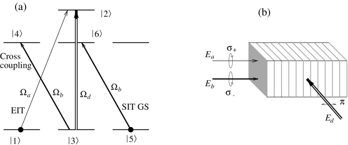
Figure 6: (a) Schematic representation of the field-atom system: The probe field $E_{a}$ exhibits EIT on the transition $\,|1\rangle\to\,|2\rangle$, in the presence of the driving field $E_{d}$ on the transition $\,|3\rangle\to\,|2\rangle$; The control field $E_{b}$ exhibits SIT GS on the transitions $\,|5\rangle\to\,|6\rangle$; The transition $\,|3\rangle\to\,|4\rangle$ serves to cross-couple the two fields. Initially only the states $\,|1\rangle$ and $\,|5\rangle$ are populated. (b) Polarizations and propagation directions of the fields involved in the transitions above.

We assume that initially all the atoms are optically pumped into the states $\,|1\rangle$ and $\,|5\rangle$, which then acquire equal populations 1/2. Hence, the sequence of transitions $\,|1\rangle\to\,|2\rangle\to\,|3\rangle\to\,|4\rangle$ repeats that of Fig. 5(a), realizing the cross-phase modulation scheme of Sec. IIIIII.1. The frequency of the $E_{a}$ field is far from the band gap frequencies of the PC, while the frequency of the $E_{b}$ field is within the band gap.

As was shown in Sec. II, PC structures doped with the near-resonant TLAs can support standing and slowly moving SIT GSs, whose pulse area (integrated over $z$) can take an arbitrarily small value. In the present setup, the transition $\,|5\rangle\to\,|6\rangle$ realizes that near-resonant TLA, allowing for slow propagation of the $E_{b}$ field through the PC.

Let us write the propagation equation for the slowly moving SIT soliton in the form

$$\Omega_{\mbox{\scriptsize SIT}}(z,t)=\Omega_{b}\text{sech}\left(\frac{tv_{g}^{(b)}-z}{2\beta}\right),$$ (26)

where $\Omega_{b}$ is the peak Rabi frequency, $v_{g}^{(b)}$ is the group velocity and $\beta=(2\alpha_{b})^{-1}$, with $\alpha_{b}$ being the absorption coefficient of the active medium at the carrier frequency $\omega_{b}$ of the soliton. The temporal width of the pulse is given by $\tau_{b}=2\beta/v_{g}^{(b)}$. The area of the $E_{b}$ pulse

$$\theta_{b}=\int_{-\infty}^{\infty}\Omega_{\mbox{\scriptsize SIT}}dt=\frac{\Omega_{b}}{v_{g}^{(b)}\alpha_{b}}\pi,$$ (27)

is then inversely proportional to the group velocity of the pulse. Hence, the SIT condition (Sec. IIIIII.1) $\theta_{b}=2\pi$ imposes a unique relation between the Rabi frequency of the SIT soliton and its group velocity:

$$v_{g}^{(b)}=\frac{\Omega_{b}}{2\alpha_{b}}.$$ (28)

The absorption-free propagation of the SIT soliton is limited to $z<v_{g}^{(b)}/\gamma_{6}$, where $\gamma_{6}$ is the decay rate of the upper atomic state $\,|6\rangle$.

Our aim is to match the group velocities of the $E_{a}$ field subject to EIT and the $E_{b}$ field having the form of a slow SIT gap soliton: $v_{g}^{(a)}=v_{g}^{(b)}$. This requires that $|\Omega_{d}|^{2}=\Omega_{b}\alpha_{a}\gamma_{2}/4\alpha_{b}$, i.e., an appropriate choice of the driving field Rabi frequency $\Omega_{d}$, for a given Rabi frequency $\Omega_{b}$ of the control field. Such velocity matching of the two copropagating weak fields would maximize their interaction.

One possibility to launch the required slow SIT soliton is to irradiate the PC by a laser beam at a small angle $\psi$ relative to the periodicity direction $z$, $\psi\simeq Dn_{0}v_{g}^{(b)}/(Lc)\ll 1$, where $D$ and $L$ are, respectively, the transverse and longitudinal dimensions of the structure. This choice of $\psi$ ensures that the $z$-component of the beam, which forms the SIT soliton and propagates in the PC with the group velocity $v_{g}^{(b)}$ over the distance $L$, will traverse the structure during the same time as the transverse component of that beam, which covers the distance $D$ with the velocity $(c/n_{0})\sin\psi$.

We have checked that for the parameter values corresponding to dopant atoms (or ions) with the mean density $N=10^{13}$ cm^-3 (surface density of $4\times 10^{8}$ cm^-2 in the thin layers), $\Delta_{b}=30\gamma_{4}$, $|\Omega_{b}|\simeq 10^{6}$ rad/s and $|\Omega_{d}|\simeq 4\times 10^{6}$ rad/s, we obtain $\pi$ phase shift of the $E_{a}$ field over a distance $z\simeq 4$ cm, while the absorption probability remains less that 10%.

Figure 7: Schematic representation of the level scheme suitable for EIT in the presence of a Raman GS (only the relevant levels are shown)

One possible difficulty of our scheme is that, with the parameters listed above, the temporal width of the $E_{b}$ field is $\tau_{b}\sim 10^{-6}$ s, and the interaction time is of the order of $10^{-3}$ s, while the lifetime of the SIT soliton is of the order of the decay time of the excited atomic state $\gamma_{6}^{-1}\sim 10^{-7}$ s. One can cope with this problem by employing the atomic level scheme shown in Fig. 7, which allows one to launch Raman solitons. We irradiate the system with an additional strong cw field $E_{R}$, which couples the $F=1$ excited state with the $F=2$ metastable ground states. The fields $E_{R}$ and $E_{b}$ are largely detuned from the fast decaying excited states $\,|4\rangle$ and $\,|6\rangle$ by an amount $\Delta\gg\gamma_{4,6}$. Then, upon adiabatically eliminating the states $\,|4\rangle$ and $\,|6\rangle$, we obtain that the Rabi frequency $\Omega_{b}$ of the control field in Eq. (26) is simply replaced by $\Omega_{b}\Omega_{R}/\Delta$. The lifetime of the SIT soliton is given now by the lifetime of the $F=2$ ground states, which can be very large, reaching in some instances a fraction of a second! In addition, such a setup allows one to launch slow Raman GSs perlin , and thus circumvent the difficulty of launching a standing (ZV) or slowly moving GSs, which must otherwise overcome the high reflectivity of the PC boundaries.

IV Conclusions

In this paper we have focused on properties of solitons in a doped PC or RABR, combining a periodic refractive-index superlattice (Bragg reflector in 1D or 2D) and a periodic set of thin active layers (consisting of TLAs resonantly interacting with the field). We have demonstrated that the system supports a vast family of bright GSs, whose properties differ substantially from their counterparts in periodic structures with either cubic or quadratic off-resonant nonlinearities. Depending on the initial conditions, these can be either standing (ZV) or slowly moving stable solitons that exhibit SIT irrespective of their photon number (pulse energy) for an appropriate group velocity. A multidimensional version of this model corresponds to a periodic set of thin active layers placed at the maxima of a 2D- or 3D-periodic refractive index. It has been found to support stable propagation of spatiotemporal solitons in the form of 2D- and 3D-localized LBs.

The best prospect of realizing a PC which is adequate for observing the GSs and LBs is to use thin layers of rare-earth ions Grei99 embedded in a spatially-periodic semiconductor structure Khit99 . The TLAs in the layers should be rare-earth-ions with the density of $10^{15}-10^{16}$ cm^-3, and large transition dipole moments. The parameter $\eta$ can vary from 0 to 100 and the detuning is $\sim 10^{12}-10^{13}$ s^-1. Cryogenic conditions in such structures can strongly extend the dephasing time $T_{2}$ and thus the soliton’s or LB’s lifetime, well into the $\mu$sec range Grei99 , which would greatly facilitate the experiment.

In a 2D PC, LBs can be envisaged to be localized on the time and transverse-length scales, respectively, $\sim 10^{-12}$ s and $1\,\mu$m. The incident pulse has uniform transverse intensity and the transverse diffraction is strong enough. One needs $d^{2}/l_{\rm abs}\lambda_{0}<1$, where $l_{{\rm abs}}$, $\lambda_{0}$ and $d$ are the resonant-absorption length, carrier wavelength, and the pulse diameter, respectively. For $l_{{\rm abs}}\sim 10^{-3}$  m and $\lambda_{0}\sim 10^{-4}$  m, one thus requires $d<10^{-4}$ m, which implies that the transverse size of the PC must be a few $\mu$m.

We have considered here (Sec. IIIIII.2) the cross-coupling of optical beams in a PC or RABR. We have pointed out, for the first time, the advantageous features of the cross coupling between EIT and SIT pulses, which is capable of producing extremely strong correlations between the two pulses. With doping parameters as above, and driving and control fields with Rabi frequencies of the order of $10^{6}$ rad/s, we can obtain a phase shift of $\pi$ for the weak probe pulse over a distance of few cm. This is much larger than any corresponding phase shift (for similar control fields) in other media.

We strongly believe that the highly promising payoff expected from the construction of suitable structures justifies the experimental challenge they pose. If and when the schemes proposed above are experimentally realized, they may prove to be useful for producing ultrasensitive nonlinear phase shifters or logical photon switches for both classical and quantum information processing or communication, owing to the unique advantages of the doped PCs over conventional EIT schemes imam ; harris_a ; harris_b ; lukin or high-Q cavities cavity_a ; cavity_b :

References

- (1) See the Photonic Band-Gap Bibliography, compiled by J. Dowling, H. Everitt, and E. Yablonovitch, at http://home.earthlink.net/~jpdowling/pbgbib.html.
- (2) E. Yablonovitch, “Inhibited spontaneous emission in solid-state physics and electronics,” Phys. Rev. Lett. 58, 2059–2062 (1987).
- (3) S. John, “Strong localization of photons in certain disordered dielectric superlattices,” Phys. Rev. Lett. 58, 2486–2489 (1987).
- (4) J. Joannopoulos, R. Meade, and J. Winn, Photonic Crystals: Molding the Flow of Light (Princeton University Press, Princeton, 1995).
- (5) P. Villeneuve, S. Fan, and J. Joannopoulos, “Microcavities in photonic crystals: Mode symmetry, tunability, and coupling efficiency,” Phys. Rev. B 54, 7837–7842 (1996).
- (6) E. Yablonovitch, T. J. Gmitter, R. D. Meade, A. M. Rappe, K. D. Brommer, and J. D. Joannopoulos, “Donor and acceptor modes in photonic band structure,” Phys. Rev. Lett. 67, 3380–3383 (1991).
- (7) A. Kofman, G. Kurizki, and B. Sherman, “Spontaneous and induced atomic decay in photonic band structures,” J. Mod. Opt. 41, 353–384 (1994).
- (8) S. John and J. Wang, “Quantum optics of localized light in a photonic band gap,” Phys. Rev. B 43, 12772–12789 (1991).
- (9) P. Lambropoulos, G. M. Nikolopoulos, T. R. Nielsen, and S. Bay, “Fundamental quantum optics in structured reservoirs,” Rep. Prog. Phys. 63, 455–503 (2000).
- (10) Z. Cheng and G. Kurizki, “Optical ’Multiexcitons’: Quantum Gap Solitons in Nonlinear Bragg Reflectors,” Phys. Rev. Lett. 75, 3430–3433 (1995).
- (11) M. Scalora, J. Dowling, C. Bowden, and M. Bloemer, “Optical limiting and switching of ultrashort pulses in nonlinear photonic band gap materials,” Phys. Rev. Lett. 73, 1368–1371 (1994).
- (12) M. Scalora, J. P. Dowling, C. M. Bowden, and M. Bloemer, “The photonic band edge optical diode,” J. Appl. Phys. 76, 2023–2026 (1994).
- (13) G. Kurizki, A. Kozhekin, T. Opatrny, and B. Malomed, “Optical solitons in periodic media with resonant and off-resonant nonlinearities,” in Progress in Optics, E. Wolf, ed., (Elsevier, North-Holland, 2001), Vol. XXXXII, pp. 93–146.
- (14) A. Kozhekin, , and G. Kurizki, “Self-Induced Transparency in Bragg Reflectors: Gap Solitons near Absorption Resonances,” Phys. Rev. Lett. 74, 5020–5023 (1995).
- (15) A. Kozhekin, , and G. Kurizki, “Standing and Moving Gap Solitons in Resonantly Absorbing Gratings,” Phys. Rev. Lett. 81, 3647–3650 (1998).
- (16) T. Opatrný, B. Malomed, and G. Kurizki, “Dark and bright solitons in resonantly absorbing gratings,” Phys. Rev. E 60, 6137–6149 (1999).
- (17) M. Blaauboer, G. Kurizki, and B. A. Malomed, “Spatiotemporally localized solitons in resonantly absorbing Bragg reflectors,” Phys. Rev. E 62, R57–R59 (2000).
- (18) D. Christodoulides and R. Joseph, “Slow Bragg solitons in nonlinear periodic structures,” Phys. Rev. Lett. 62, 1746–1749 (1989).
- (19) A. Aceves and S. Wabnitz, “Self-induced transparency solitons in nonlinear refractive periodic media,” Phys. Lett. A 141, 37–40 (1989).
- (20) J. Feng and F. Kneubuhl, “Solitons in a periodic structure with Kerr nonlinearity,” IEEE Journal of Quantum Electronics 29, 590 (1993).
- (21) C. de Sterke, , and J. E. Sipe, “Gap solitons,” in Progress in Optics, E. Wolf, ed., (Elsevier, North-Holland, 1997), Vol. XXXIII, Chap. 3, pp. 205–259.
- (22) B. Eggleton, R. Slusher, C. de Sterke, P. Krug, and J. Sipe, “Bragg grating solitons,” Phys. Rev. Lett. 76, 1627–1630 (1996).
- (23) S. McCall and E. Hahn, “Self-induced transparency by oulsed coherent light,” Phys. Rev. Lett. 18, 908–911 (1967).
- (24) S. McCall and E. Hahn, “Self-induced transparency,” Phys. Rev. 183, 457–485 (1969).
- (25) N. Aközbek and S. John, “Self-induced transparency solitary waves in a doped nonlinear photonic band gap material,” Phys. Rev. E 58, 3876–3895 (1998).
- (26) B. Mantsyzov, “Gap pulse with an inhomogeneously broadened line and an oscillating solitary wave,” Phys. Rev. A 51, 4939–4943 (1995).
- (27) A. Newell and J. Moloney, Nonlinear Optics (Addison-Wesley, Redwood City CA, 1992).
- (28) Y. Silberberg, “Collapse of optical pulses,” Opt. Lett. 15, 1282–1285 (1990).
- (29) M. Blaauboer, G. Kurizki, and B. A. Malomed, “Spatiotemporally localized multidimensional solitons in self-induced transparency media,” Phys. Rev. Lett. 84, 1906–1909 (2000).
- (30) T. W. Mossberg, “Time-domain frequency-selective optical data storage,” Opt. Lett. 7, 77–79 (1982).
- (31) S. Harris, “Electromagnetically induced transparency,” Phys. Today 50, 36–42 (1997).
- (32) M. Scully and M. Zubairy, in Quantum Optics (Cambridge University Press, Cambridge, 1997), Chap. 7.
- (33) H. Schmidt and A. Imamoğlu, “Giant Kerr nonlinearities obtained by electromagnetically induced transparency,” Opt. Lett. 21, 1936–1938 (1996).
- (34) S. Harris and Y. Yamamoto, “Photon switching by quantum interference,” Phys. Rev. Lett. 81, 3611–3614 (1998).
- (35) S. Harris and L. Hau, “Nonlinear optics at low light levels,” Phys. Rev. Lett. 82, 4611–4614 (1999).
- (36) H. G. Winful and V. Perlin, “Raman Gap Solitons,” Phys. Rev. Lett. 84, 3586–3589 (2000).
- (37) C. Greiner, B. Boggs, T. Loftus, T. Wang, and T. Mossberg, “Polarization-dependent Rabi frequency beats in the coherent response of tm3+ in YAG,” Phys. Rev. A 60, R2657–R2660 (1999).
- (38) G. Khitrova, H. Gibbs, F. Jahnke, M. Kira, and S. Koch, “Nonlinear optics of normal-mode-coupling semiconductor microcavities,” Rev. Mod. Phys. 71, 1591–1640 (1999).
- (39) M. Lukin and A. Imamoğlu, “Nonlinear optics and quantum entanglement of ultraslow single photons,” Phys. Rev. Lett. 84, 1419–1422 (2000).
- (40) H. Kimble, “Strong interaction of single atoms and photons in cavity QED,” Phys. Scr. 76, 127–137 (1998).
- (41) A. Imamoğlu, H. Schmidt, G. Woods, and M. Deutsch, “Strongly interacting photons in a nonlinear cavity,” Phys. Rev. Lett. 79, 1467–1470 (1997).