Controlling quantum entanglement through photocounts
Abstract
We present a protocol to generate and control quantum entanglement between the states of two subsystems (the system ) by making measurements on a third subsystem (the monitor ), interacting with . For the sake of comparison we consider first an ideal, or instantaneous projective measurement, as postulated by von Neumann. Then we compare it with the more realistic or generalized measurement procedure based on photocounting on . Further we consider that the interaction term (between and ) contains a quantum nondemolition variable of and discuss the possibility and limitations for reconstructing the initial state of from information acquired by photocounting on .
I Introduction
Information processing can be largely improved when quantum properties are used for encoding both, bits and channels [1]. While bits are encoded in mutually orthogonal states of a quantum system, quantum channels use the ability to set systems in entangled states. Entanglement of states is a characteristic quantum correlation that, in principle, can be produced in post interacting quantum systems [2]. To use this quantum resource for information processing one has to be able first to produce and then to control the amount of entanglement of a finite number of quantum systems. A fundamental open problem in quantum information is the characterization and classification of mixed entangled states of a multipartite systems [3]. Nowadays the most accessible and controllable source of quantum entanglement has been the electromagnetic field, through parametric down-conversion processes in non-linear crystals [4, 5]. Recently, internal atomic states entanglement have also been considered in distinct experiments [6, 7, 8, 9].
We propose a consistent scheme for generating and controlling entangled states of two subsystems (that we call ): (i) If the subsystems do interact, their initial states should be adequately prepared such that the interaction does not entangle their states during the time evolution. (ii) A third quantum subsystem, the monitor , is coupled (through ) to ; should be the only subsystem responsible for entangling the states of , thus formally, is a necessary condition. Then follows an operational procedure or protocol: (iii) First one choose an observable of and after an elapsed time , from the beginning of the interaction (between and ), it is measured and the interaction is turned off; the eigenvalue outcome determines the entangled state in which is left.
In an ideal projective measurement the measured eigenvalues occur with a certain probability, so the entangled state of obtained through reduction, cannot, in principle, be chosen. However, if the experimentalist is able to control the outcomes of to be read, then, controlling the degree of entanglement in becomes possible and the protocol becomes feasible. Interestingly, in a realistic measurement, when quanta are counted, it is possible to control the outcome of the monitor: One turns on the interaction between and and when quanta are counted then one knows in which state the system is left. However, the necessary interval of time for counting quanta is probabilistic: if the experiment is repeated, the same number of quanta may be registered within another time interval. Thus, for reproducing the same state one should repeat the experiment such that the counted photons be the same within the same time interval. The present status for generating entangled states is very different from this protocol, the experiments are based on projective measurements [4, 5].
The realization of the proposed scheme and protocol are considered in the following physical system: the subsystems constituting may consist of two interacting (but not necessarily) electromagnetic (EM) fields, modes A and B, coupled to the monitor , a third EM field, the mode C. The entanglement in is created by a continuous destructive photocount on C and the control is fulfilled by turning off the interaction when a certain predetermined number of photons become registered, thus the system is left in an entangled state which is essentially characterized by . This proposal is detailed in the following sections: In Sec. II we present our model and write the Hamiltonian for the system , the monitor and their interaction, we also give the time-dependent state vector of the whole system. In Sec. III we describe the measurement process in two different approaches for sake of comparison, the ideal and the realistic: (i) The ideal or instantaneous projective measurement on field C, assumes the statevector reduction by projection as postulated by von Neumann, leading to an entangled (regarding the fields A and B) pure states. (ii) Then, more realistically, we consider the measurement as a sequential photocount process, on field C, as proposed by Srinavas and Davies [10]. This leads to an entangled density operator for fields A and B. We show that only the second approach allows controlling the degree of entanglement of the AB fields, depending on the detector counting rate (), the number of counted photons () and counting time. In Sec. IV we show that due to the nondemolishing character of the coupling between and , the total photon number of can be inferred (without altering ) by averaging over counted photons of mode C. We also analyze the information one gets about the initial state of from the counting process on ; examples are presented and discussed. In Sec. 5 we present a summary and conclusions.
II Model
The problem of production and control of state entanglement between two subsystems is based on the physical paradigm of four interacting EM fields. Couplings of EM modes are made possible in nonlinear media and phenomena such as parametric down and up conversion appearing when a response of second order nonlinearity in crystal polarization is present and four-wave mixing (third order nonlinearity) occurs in a Kerr medium [11]. Also, recently a strong field-field interaction of few photons, induced by non-resonant interactions between fields and a Cs atom, was observed experimentally [12]. This observation led to a proposal for attaining high-nonlinearities with single atoms [13]. The dynamics of the fields here considered consists of two processes: (i) a second order nonlinear process coupling the modes A and B (), assisted by a classical pump field [14, 15] and (ii) a four-wave mixing, with modes, A, B and C (treated as quantized fields) coupled to a fourth classical intense field. The system dynamics is described by the Hamiltonian
| (2) | |||||
The total number of photons of modes A and B, is a quantum nondemolition (QND) variable. This is a quite important feature because while measuring (destructively) the mode C, an inference can be made on , without loosing or altering a single quanta of modes A and B. It has been shown that the coupling between A and B as in Hamiltonian (2) displays several interesting features [16]: (i) It leads to a complete states swapping (information exchange) even at constant mean energy. (ii) If the states are initially not entangled, the interaction will produce entanglement only if one of the modes is prepared in a nonclassical state; otherwise, if both modes are initially prepared as a direct product of coherent states the interaction will not change this character in the course of their evolution [2].
In the interaction picture, Hamiltonian (2) is written as
| (3) |
where, resonance conditions, and , must be satisfied in order to eliminate the explicit time dependence present in (2).
Next, suppose the monitor mode C (the meter in the terminology of [17]) is prepared in the vacuum state, so, during its evolution it could absorb energy only from the intense classical field. The fields A and B are considered, for the moment, to be in an arbitrary state, that we write as an expansion in the number states basis and , (from here on we omit the subscript ). At time the evolved state of the AB system is represented by
| (4) |
Noting that is a coherent state restricted to the imaginary axis, state (4) can be written as
| (5) |
(here on we omit the subscript C) where . In the next section we discuss two forms of measurements on mode C.
III Monitoring AB fields trough measurement on C
A Instantaneous projective measurement
An ideal or instantaneous projective measurement (PM) of a system is associated to a chosen observable (or a set of commuting observables) of this system. If at time one of the eigenvalues of is realized, then the system state is reduced to its corresponding eigenvector . The probability for that realization is . This is known as a measurement of the first kind, as postulated by von Neumann. In our model, if at time it is found that field C contains exactly photons, the state is automatically projected on to the number state . As a consequence, the AB joint state ‘reduces’ instantaneously to the new state
| (6) |
where and stands for the trace operation on the A and B fields operators. The probability that at time the field C has quanta is Tr. For the state given by equation (5) this probability is
| (7) | |||||
| (8) |
the second equality follows because , so the counts are independent of the evolution of AB modes, they are not affected by the evolution of the AB system. The evolved state is reduced to
| (9) |
or in terms of the statevector (excepting a phase factor),
| (10) |
the purity of the state is maintained, however, entanglement is created even if initially the state is factorized.
The mean photon number of field C is closely related to the mean of AB fields,
| (11) |
so, a measurement on C allows to infer the mean squared QND variable with a proportionality factor that goes as . The variances are related as
| (12) |
where .
If fields A and B are initially prepared in number states, , the reduced state of the AB field becomes independent of , evolving freely as
| (13) |
thus, not feeling at all the presence of field C; so, any entanglement will only arise from the interaction between A and B and not from a measurement on C. The probability for measuring photons in C at time will depend on and as , the probability distribution being Poissonian
| (14) |
The mean photon number of C Eq. (11) gives
| (15) |
whereas
| (16) |
Inversely, if one ignores in which states the AB modes were prepared, but however verifies, through a measurement on C, that , then one immediately infers that the AB system was prepared in some number state . If the modes A and B are prepared in eigenstates of the QND variable the subsystem AB evolves independently of C.
Now, if the initial states of the subsystems A and B are prepared as a direct product of coherent states, , the unitary evolution does not entangle the states of A and B, each one continues its evolution as such,
| (17) |
where , with and (note that is a constant of the motion). Although the measurement on C affects the dynamics of the AB system by entangling the states, this very ideal measurement does not allow controlling the entanglement dynamics of the AB system, since the outcome of the eigenvalue is probabilistic, according to the distribution (8).
As in the previous case, the mean photon number of C will depend on time as ,
| (18) |
the variance is given by
| (19) |
and can be obtained from the measurements on ,
| (20) |
where the right hand side, calculated from the experiment should be time-independent.
B Generalized measurement by photocounting
Experiments involving counting are not instantaneous and far from the von Neumann idealization. For a realistic counting measurement, one should consider that (i) For a given time interval the counting of quanta occurs with some probability, or, it is not likely that exactly quanta are counted in a predefined time , actually, there will be a distribution of time intervals. (ii) More importantly, one has to consider that when one photon is counted the EM field will have one photon less. The dynamics of this kind of process has to be treated as a dissipative continuous measurement; this subject was well addressed by Srinavas and Davies [10] and applied to several situations in [17, 18, 19]. We follow closely these references, describing the continuous photocount measurement in the formalism of operations and effects [20].
The count of photons from the monitor mode in a time is characterized by the linear operation , acting on the state of the system,
| (21) |
where is the state of the ABC system prior turning on the counting process and is the probability of counting photons in . The linear operator is written in terms of two other operators, and ,
| (22) |
where is a superoperator defined in terms of ordinary Hilbert space operators as
| (23) |
is a semigroup element given in terms of the generator as . As defined in [10] the generator is
| (24) |
where is the system Hamiltonian and is the rate operator given by
| (25) |
and the parameter stands for the detector counting rate. The theory becomes self contained by choosing as
| (26) |
standing for the change of the field C due to loss of one counted photon and is responsible for the state evolution between counts.
In the interaction picture becomes
| (27) |
the first term contributes only to the free evolution of the AB fields as a unitary evolution of the initial state. The monitor field stands for the counting process, being present in the other terms, thus the linear superoperator , acting on the initial state , can be expressed as
| (28) |
where
| (29) |
with
| (30) | |||||
| (31) |
We have defined as the superoperator for the coherent evolution of modes A and B
| (32) |
After doing some algebraic manipulations we find that for counts on C the state for the ABC system becomes
| (34) | |||||
where , is the label of the coherent state and . and stand for the same expressions but with instead of . The normalization function is the probability for counted photons in time ,
| (35) |
the same as in the ideal PM, Eq. (8), however the factor is now replaced by . An important difference arises here, for we have , the time appearing linearly while in the ideal PM it is quadratic. The expressions for the mean and variance of are as (18) and (19) however with substituting .
The mixed state is a post-measurement state for counting photons. The pre-measurement state is obtained by summing over all the possible outcomes, [19].
The state of the AB system is obtained by tracing over the monitor mode,
| (37) | |||||
where , and
| (38) |
Preparing the modes A and B in number states the mode C has its dynamical evolution decoupled from the AB system. As in the ideal PM, Eq. (13), the AB modes states evolve freely, not being affected at all by the counting process (due to the QND variable).
For the modes A and B prepared in coherent states, , the unitary evolution does not change this character, each state continues to evolve as such (), however, the photocount on C affects the dynamics introducing a another effect: besides the entanglement, as in the ideal PM, the factor in brackets in (37) mixes the states. The number of counted photons in mode C determines the selection of a specific entangled state of the AB field and the degree of its entanglement. This will depend on , the counting rate of the detector , the number of counts , the time , and there will also be a dependence on the initial state through the total number of photons operator . So, controlling these quantities entails the correlated state (37). It is worth stressing that time interval for counting exactly photons is probabilistic and is its (non-normalized) distribution function.
C Degree of entanglement and mixing
It is well known that a precise measure of the degree of entanglement is not available for continuous variables mixed states [3]. We saw that a straightforward application of the photocount measurement process, may be used for producing and determining the degree of a -entangled state of AB modes. Formally, for the AB system, prepared initially in coherent states, the dissipative (nonunitary) character of the evolution is induced by the counting process, being responsible for the interplay between the entanglement, mixing and decoherence in (37).
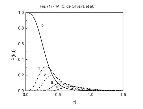
For the lowest values of the probability distributions are depicted in Fig. 1 for . One perceives that for the highest values of the probability occur for , however for the probabilities attain maximum values at different times . For one has , and , so state (37) does not mix substantially for small time intervals, it can be written as
| (39) |
(here, ) and, excepting for (), the counting process generates entanglement.
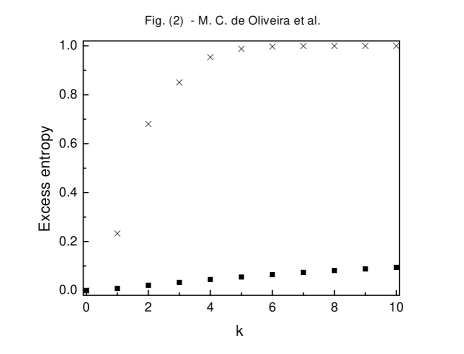
Comparing state (39) with (17) for , we see that they are very likely, thus for small times they cannot be distinguished and the entanglement will be stronger the higher the number of counted photons. We give a quantitative picture of entanglement by calculating the excess entropy [21], defined as
| (40) |
where () is the entropy of the mode A (B)(associated to ) and is the entropy of the AB system, where . The excess entropy measures the information contained in the correlation between modes A and B. Its lower and upper bounds are obtained by the Araki-Lieb [22] inequality
| (41) |
namely,
| (42) |
Remark that measures the correlation between A and B, without resolving between classical or quantum correlation (entanglement). However, when the joint system is in a pure state and , the inequality (42) reduces to
| (43) |
and any correlation given by will be due to entanglement. Thus, the measure of together with the system degree of purity allows one to distinguish between classes of entangled states, even though it does not give a precise borderline for separability of mixed entangled states.
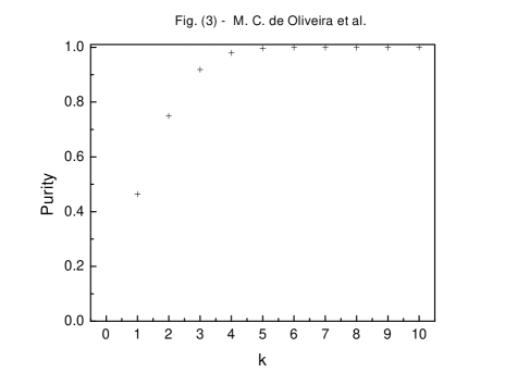
The excess entropy for the system here considered is plotted in Fig. 2 as function of for most probable time of a -event (crosses for (37)) and for initial times () (filled squares for (39)). It is verified that the counts correlate the subsystems more intensely the higher is the number of counted photons. Since state (39) is pure (), this correlation characterizes a maximal entanglement. When detections occur at initial time the state of the joint system AB is left in a pure entangled state and the degree of entanglement is directly proportional to the number of counted photons. The excess entropy for state (37) is calculated at times (for which is maximum - as in Fig. 1) and one sees that the correlation is stronger than for state (39). However, as state (37) is mixed one also need to measure its purity (), as depicted in Fig. 3, for several values of and at times . The combined results of Figs. 2 and 3 for the mixed state entanglement, show that the higher the number of counted photons, the more correlated becomes the AB state, and for one has . However, the states more likely to occur at times are not pure anymore and for high ’s, characterized by and , the state (37) becomes classically correlated (separable), while for it is non-separable, which characterizes non-maximal entanglement.
How this process happens can be represented by the following example, which exactly matches our results for both the excess entropy and purity. Considering the condition of separability,
| (44) |
with acting on ; and , then,
| (45) |
When
| (46) |
one obtains
| (47) |
For (as it is for coherent states) both quantities go to . So, for a sufficiently large the state (37) becomes separable. State (44) (together with (46)) corresponds to an equiprobable ensemble of states.
In that way, we saw that a full range of states may be generated, with different degree of entanglement, from maximally entangled to separable states. So, the protocol for producing a specific state (37) consists in turning off the interaction when an a priori selected value is attained at a time .
Besides, the photocount measurement theory and the specific Hamiltonian (3) also allow to extract information about the AB system by counting the photons of C. Due to the nature of the coupling between the monitor and the AB system, the counting on C gives the maximal information about any function of . Then it is immediate to put the question: How much information may the photocount distribution give about the initial quantum states ? This is discussed bellow.
IV Probing light with light
Here we look at the counting problem as a spectroscopic measure of the state of the AB system. Light state spectroscopy, or light probing via atomic deflection was discussed by M. Freyberger and A. M. Herkommer [23]. Probability distribution of transversal momenta of two-level atoms deflected by an EM field in a cavity allows the complete knowledge of the field quantum state. Is it possible to use a similar strategy with fields only, but now instead of the beam deflection, the photocount playing the role revealing the AB state?
To make this point clear let us consider the average counted photon number
| (48) |
where . For , and we can write
| (49) |
and can be inferred directly by the mean counted photons, this being more precise the larger is because one gets a linear relation between time and . This point was actually pointed by Milburn and Walls [17] for a single mode coupled to C. Note that differently from the projective measurement where increases with , Eq. (15), in the non-ideal measurement increases linearly with time. We can build up higher-order moments of in a similar fashion, obtaining,
| (50) |
or keeping only the higher power in for conveniently chosen time , we have
| (51) |
Calling
| (52) |
multiplying both sides of the above equation by () and summing over we get a new function, which a Fourier expansion of the squared moduli coefficients,
| (53) |
which is always bounded, with values in the interval since . The left hand side is calculated from the experimental photocounts, thus a specific relation between a particular set of the may be inferred in certain cases, as to be see below. Doing an inverse Fourier transform we get
| (54) |
which is the only information on the initial state of the AB system one gets by photocounting on C. If the fields A and B are initially disentangled, , then in order to determine the coefficients of, for instance, the initial state of mode A, , one should set the initial state of B in the vacuum state (or any other number state), since and all other coefficient being zero, so one obtains
| (55) |
This strategy has its limitation since only the moduli of the coefficients can be obtained, being the maximum information about the initial state of field A that one can obtain by counting on C.
Particularly interesting states to be addressed are the initially entangled states.
(a) We first consider the case when both modes are prepared in the superposition of perfect anti-correlation
| (56) |
defined as a limited sum of the photon number state, and . One illustrative example of this kind of state is for entangled qubits (), .
For state (56) the probability of counting photons is independent of the coefficients ,
| (58) | |||||
so, all higher moments are determined from the first one, the mean counted photons is a precise measurement since the variance is zero and consequently the squared coefficients cannot be determined. For the expression for the -moments (expressed as , see (52)) of counted photons will be
| (59) |
(b) Now, let us consider the case when both modes are prepared in the superposition of perfect correlation
| (60) |
Again, for qubits, . For the state (60) the probability of counting photons is
| (62) | |||||
and for the moments of counted photons (expressed in terms of ) will be
| (63) |
and all coefficients squared moduli can be determined,
| (64) |
When and
| (65) |
state (60) is a two-mode squeezed state ( is the squeezing parameter) used to establish the quantum channel for the continuous variable teleportation, as reported in [24]. So, all terms can be precisely determined since all depend on the parameter that can be inferred from the relations between the coefficients.
V Summary and concluding remarks
We have considered a monitor subsystem (an EM mode, C) coupled to a system of interest , (two interacting modes, A and B), where the interacting term in the hamiltonian contains a QND variable of : the total quanta of modes A and B. We proposed a nondeterministic entanglement generation protocol of the two modes, A and B, based on the continuous photodetection theory. By counting destructively photons of the mode C the amount of entanglement of the joint state of modes AB, prepared initially in coherent states, can be controlled. Due to the dissipative character of the non-ideal photodectection model, nonmaximally entangled states (mixtures) are generated. The distribution function for counting photons and time intervals is well defined allowing the determination of the most probable time for the occurrence for each value of .
For the sake of comparison we also investigated the case of an ideal or projective measurement (instantaneous) as discussed by von Neumann. The projection of the state in a photon number operator eigenstate pure entangled of A and B, however no control can be done, because the realization of eigenstate cannot be fixed a priori, it occurs probabilistically.
The post-selected counting distribution function allows calculating the moments of the counted photons of C, which, for are closely related to the moments of the squared number of photons of both modes, , which is a constant of the motion. So, also higher moments of can be inferred in a nondemolition measurement. This has a immediate use, as probing the state of the AB system by means of the counting distribution function. Examples were given, and as expected, the extracted information showed to be useful for partial or total reconstruction of the initial state of modes A and B. Since only the squared modulus of the coefficients of the state are given, we remarked that such procedure is not able to distinguish systems between pure or mixed states prepared as maximally entangled.
Although the system here discussed is constituted of EM field modes, the couplings may possibly be realized in other systems such as vibrational degrees of freedom of trapped ions [25] or even Bose-Einstein condensates [26]. In both cases the coupling of the atomic system with a light field (monitor mode) is able to entangle atomic systems. It is also possible to probe the atomic system state by photocounting on a light beam. In such cases we expect collisions to be important if not restrictive to the method. An obvious extension of the protocol here proposed is to use the classical information achieved to control the AB system state in a continuous feedback process [27]. This allows the coherent control of state entanglement of systems, and would be, indeed, useful for quantum information processing [1].
ACKNOWLEDGMENTS
This work was supported by FAPESP under contract 00/15084-5. MCO acknowledges FAPESP São Paulo) for total financial support; LFS acknowledges total financial support from CAPES (Brasília) and SSM acknowledges partial financial support from CNPq (Brasília).
REFERENCES
- [1] M.A. Nielsen and I.L. Chuang Quantum Computation and Quantum Information (Cambridge University Press, UK,2000).
- [2] M.C. de Oliveira and W.J. Munro Quantum resources and information exchange in deterministic entanglement formation, submitted for publication.
- [3] M. Lewenstein, B. Kraus, P. Horodecki, and J.I. Cirac, Phys. Rev. A 63, 044304 (2001)
- [4] P.G. Kwiat, K. Mattle, H. Weinfurter, A. Zeilinger, A.V. Sergienko, and Y. Shih, Phys. Rev. Lett. 75, 4337 (1995).
- [5] A.G. White, D.F.V. James, P.H. Eberhard, and P.G. Kwiat, Phys. Rev. Lett. 83, 3103 (1999).
- [6] E. Hagley, X. Maître, G. Nogues, C. Wunderlich, M. Brune, J. M. Raimond, and S. Haroche, Phys. Rev. Lett. 79, 1 (1997).
- [7] A. Rauschenbeutel, G. Nogues, S. Osnaghi, P. Bertet, M. Brune, J.M. Raimond, and S. Haroche, Science 288, 2024 (2000).
- [8] C.A. Sackett, D. Kielpinski, B.E. King, C. Langer, V. Meyer, C.J. Myatt, M. Rowe, Q.A. Turchette, W.M. Itano, D.J. Wineland, and C. Monroe, Nature 404, 256 (2000).
- [9] B. Julsgaard, A. Koxhekin, and E.S. Polzik, Nature 413, 400 (2001).
- [10] M.D. Srinavas and E.B. Davies, Opt. Acta 28, 981 (1981).
- [11] A. Yariv, Quantum Electronics, (John Wiley & Sons, USA, 1989).
- [12] Q.A. Turchette, C.J. Hood, W. Lange, H. Mabuchi, and H.J. Kimble, Phys. Rev. Lett. 75, 4710 (1995).
- [13] S. Rebic, S. M. Tan, A. S. Parkins, and D.F. Walls, J. Opt. B 1, 490 (1999).
- [14] D. F. Walls and G. J. Milburn, Quantum Optics, (Springer-Verlag, Berlin, 1995).
- [15] M. O. Scully and M. S. Zubairy Quantum Optics, (Cambridge University Press, UK) 1997
- [16] M.C. de Oliveira, V.V. Dodonov and S.S. Mizrahi, J. Opt. B 1, 610 (1999).
- [17] G.J. Milburn and D.F. Walls, Phys. Rev. A 30, 56 (1984).
- [18] C.A. Holmes, G.J. Milburn, and D.F. Walls, Phys. Rev. A 39, 2493 (1989).
- [19] C.M. Caves and G.J. Milburn, Phys. Rev. A 36, 5543 (1987).
- [20] K. Kraus, States, Effects, and Operations (Springer-Verlag, Berlin, 1984).
- [21] G. Lindblad, Non-equilibrium entropy and irreversibility, (Reidel,Dordrecht,1983).
- [22] H. Araki and E.H. Lieb, Commun. Math. Phys. 18, 160 (1970).
- [23] M. Freyberger and A.M. Herkommer, Phys. Rev. Lett. 72, 1952 (1994).
- [24] A. Furusawa, J.L. Sørensen, S.L. Braunstein, C.A. Fuchs, H.J. Kimble and E.S. Polzik, Science 282, 706 (1998).
- [25] J. Steinbach, J. Twamley, and P.L. Knight, Phys. Rev. A 56, 4815 (1997).
- [26] A.S. Parkins and D.F. Walls, Phys. Rep. 303, 1 (1998).
- [27] H.M. Wiseman, Quantum Trajectories and Feedback(Phd Thesis, 1994).
figures