Quantum Jumps, EEQT and the Five Platonic Fractals

Abstract

It is shown that symmetric configurations of fuzzy spin direction detectors generate, through quantum jumps, IFS fractals on the sphere $S^{2}.$ The IFS fractals can be also interpreted as resulting from applications of Lorentz boosts to the projective light cone.

1 Introduction

Recently, Numerical Algorithms for quantum jumps were discovered. First they were introduced in quantum optics as convenient and effective tools for numerical simulations of the Liouville equation [1, 2, 3, 4]. A short history and more references can be found in Ref. [5]. Ph. Blanchard and A. Jadczyk, in a series of papers on EEQT - Event Enhanced Quantum Theory (cf. [6, 7, 8, 9, 10, 11] and references therein) - developed a new approach that unifies what John von Neumann called U- and R-processes [12] into a single piecewise deterministic process (PDP) where continuous evolution of a system is cyclically interrupted by discontinuous ”jumps”.

Normally one would expect that time evolution of a physical system is described by a differential equation. That is how laws of physics are usually expressed. Here however we have a surprise: in EEQT a history of an individual quantum system, coupled to a monitoring device, as in every real world experiment, is described by a process  or an algorithm  rather than by a differential equation. The PDP is similar to those studied in the science of economics, where periods of smooth fluctuations are interrupted by market crashes [13, 14]. A quantum jump is what corresponds to a market crash - a discontinuity, a ’catastrophe’. But discontinuities and catastrophes have their own laws, and here comes the concept of a piecewise deterministic Markov process - a PDP.

PDPs are the simple and elegant ways to describe the world in terms of cyclic, rather than linear, time; that is the world of cyclically, though somewhat irregularly, recurring catastrophes. In the cases studied in the present paper the catastrophes come from the coupling of a quantum system to a system of two-state ”detectors”. In this case the catastrophes are not really catastrophes for the detectors - detectors just flip, which is exactly what detectors do for living. But these flips bring catastrophes for the quantum system, because with each flip of the detector, with each ”event”, as we call it, the quantum system state vector breaks its continuous evolution, and instantaneously jumps to a different state - it ”rejuvenates” and it starts another cycle of a peaceful, continuous evolution - till the next catastrophe.

Note. The term instantaneously in the last sentence may suggest that our formalism is incompatible with Einstein’s relativity. That this is not so has been demonstrated in Ref.[10] (for a somewhat different approach cf also [15, 16, 17]). The point is that for a relativistic theory the role of time is being played by the Fock-Schwinger ”proper time” as a Floquet variable. The reader should bear in mind that the EEQT algorithm is explicitly nonlocal: to simulate a history of an individual system integrations over entire space (or space-time) are needed.

The EEQT algorithm generating quantum jumps is similar in its nature to a nonlinear iterated function system (IFS) [18] (see also [19] and references therein) and, as such, it generically produces a chaotic dynamics for the coupled system. Here the probabilities assigned to the maps are derived from quantum transition probabilities and thus depend on the actual point, but such generalizations of the IFS’s have been also studied (cf. [20] and references therein). In the present paper we describe the algorithm generating quantum fractals, that is self-similar patterns on the projective plane $\mathbb{P}_{1}({\mathbb{C}})\approx S^{2}$, when a continuous in time ”measurement” of several spin directions at once takes place.

Note: The term quantum fractals has been used before by Casati et al. [21, 22] in a different context.

Note: The operators for different spin directions do not commute, but this does not contradicts Heisenberg’s uncertainty relations as these deal with statistical ensembles averages, while here we are describing an individual quantum system. In fact, realizing the chaotic behavior of a quantum state vector, when several noncommuting observables are being simultaneously monitored, can help us to understand the mechanisms of statistical uncertainties.

As stated above the algorithm of EEQT describes a piecewise deterministic random process - periods of a smooth evolution interspersed with catastrophic ”jumps.” Of course, once we have individual description, we can also get the laws for statistical ensembles. Here we get a nice, linear, Liouville evolution equation for measures - as it is usual in studying chaotic dynamics. The fact that there is a unique PDP generating the Liouville equation in the framework of EEQT has been proven in Ref. [23].

2 EEQT - Quantum Fractals

2.1 Geometry

We have published, as an OpenSource project [24], the algorithm implemented in Java that generates the Five Platonic Fractals - that is fractals generated by five most symmetric detector configurations. The algorithm generates self-similar patterns on a sphere of a unit radius. The points on the sphere represent (pure) states of the simplest quantum system - the spin $1/2$ rotator. This spin $1/2$ quantum system is coupled, continuously in time, to a finite number of symmetrically distributed spin-direction detectors. Thus the symmetry of the pattern reflects the symmetry of the detector directions distribution. Each spin direction is characterized by a vector ${\bf n}$ of unit length. Here we study the most symmetrical configurations, therefore we chose direction vectors ${\bf n}_{i}$ pointing from the origin to the vertices of one of the five platonic solids. We consider the following five detectors configurations:

1. tetrahedron: 4 detectors along the directions ${\bf n}[i],i=1,\ldots,4$
   {{0, 0, 1.}, {a[17], 0, -a[3]}, {-a[6], a[12], -a[3]}, {-a[6], -a[12], -a[3]}}

2. octahedron: 6 detectors along the directions ${\bf n}[i],i=1,\ldots,6$
   {{0, 0, 1.}, {1., 0, 0}, {0, 1., 0},
   {-1., 0, 0}, {0, -1., 0}, {0, 0, -1.}}

3. cube: 8 detectors along the directions ${\bf n}[i],i=1,\ldots,8$
   {{0, 0, 1.}, {a[17], 0, a[3]}, {-a[6], a[12], a[3]}, {-a[6], -a[12], a[3]},
   {a[6], a[12], -a[3]}, {a[6], -a[12], -a[3]}, {-a[17], 0, -a[3]}, {0, 0, -1.}}

4. icosahedron: 12 detectors along the directions ${\bf n}[i],i=1,\ldots,12$
   {{0, 0, 1.}, {0.a[15], 0, a[5]}, {a[2], a[13], a[5]}, {-a[10], a[7], a[5]},
   {-a[10], -a[7], a[5]}, {a[2], -a[13], a[5]}, {a[10], a[7], -a[5]},
   {a[10], -a[7], -a[5]}, {-a[2], a[13], -a[5]}, {-a[15], 0, -a[5]},
   {-a[2], -a[13], -a[5]}, {0, 0, -1.}}

5. dodecahedron: 20 detectors along the directions ${\bf n}[i],i=1,\ldots,20$
   {{0, 0, 1.}, {a[9], 0, a[11]}, {-a[3], a[8], a[11]}, {-a[3], -a[8], a[11]},
   {a[11], a[8], a[3]}, {a[11], -a[8], a[3]}, {-a[14], a[4], a[3]},
   {a[1], a[16], a[3]}, {a[1], -a[16], a[3]}, {-a[14], -a[4], a[3]},
   {a[14], a[4], -a[3]}, {a[14], -a[4], -a[3]}, {-a[11], a[8], -a[3]},
   {-a[1], a[16], -a[3]}, {-a[1], -a[16], -a[3]}, {-a[11],  -a[8], -a[3]},
   {a[3], a[8], -a[11]}, {a[3], -a[8], -a[11]}, {-a[9], 0, -a[11]},
   {0, 0, -1.}}

where the array of real numbers $a[i],\/i=1,\ldots,17$ is given in the following table.

$a[1]=\frac{3-\sqrt{5}}{6}$	$a[2]=\frac{5-\sqrt{5}}{10}$	$a[3]=\frac{1}{3}$	$a[4]=\frac{\sqrt{5}-1}{2\sqrt{3}}$
$a[5]=\frac{1}{\sqrt{5}}$	$a[6]=\frac{\sqrt{2}}{3}$	$a[7]=\sqrt{\frac{5-\sqrt{5}}{10}}$	$a[8]=\frac{1}{\sqrt{3}}$
$a[9]=\frac{2}{3}$	$a[10]=\frac{5+\sqrt{5}}{10}$	$a[11]=\frac{\sqrt{5}}{3}$	$a[12]=\sqrt{\frac{2}{3}}$
$a[13]=\sqrt{\frac{5+\sqrt{5}}{10}}$	$a[14]=\frac{3+\sqrt{5}}{6}$	$a[15]=\frac{2}{\sqrt{5}}$	$a[16]=\sqrt{\frac{3+\sqrt{5}}{6}}$
$a[17]=\frac{2\sqrt{2}}{3}$

Note: There is no deep reason why we chose these configurations - simplicity and beauty are the main factors here. Notice that, to enable easy zooming onto the attractor, we have chosen the orientations in such a way that in each case the North Pole, with coordinates (0,0,1), of the sphere is occupied by one of the vertices.

2.2 The algorithm

Here we describe the algorithm. Comments on its meaning and on the derivation can be found in the endnotes in Section 4

2.2.1 The Hilbert space

The quantum system is represented in a two-dimensional complex Hilbert space, which we realize as ${\mathbb{C}}^{2}$ - the set of all column vectors

$$a=\pmatrix{a_{1}\cr a_{2}}$$ (1)

where $a_{1}$ and $a_{2}$ are complex numbers, and with scalar product $(a,b)$ defined by

$$(a,b)={\bar{a}}_{1}b_{1}+{\bar{a}}_{2}b_{2}$$ (2)

where the bar ${\bar{c}}$ stands for the complex conjugation of the complex number $c.$

2.2.2 Spin directions

We choose the Pauli matrices $\sigma_{x},\sigma_{y},\sigma_{z}$ to represent spin directions along $x,y,z$ axes respectively.

$$\sigma_{1}=\sigma_{x}=\pmatrix{0,&1\cr 1,&0},\quad\sigma_{2}=\sigma_{y}=\pmatrix{0,&-{\mathrm{i}}\cr{\mathrm{i}},&0},\quad\sigma_{3}=\sigma_{z}=\pmatrix{1,&0\cr 0,&-1}$$

Together with the identity matrix

$$\sigma_{0}=I=\pmatrix{1,&0\cr 0,&1}$$ (3)

they span the whole $2\times 2$ complex matrix algebra. In computations it is important to make use of the fact that Pauli matrices (after multiplication by ”-i”) represent the quaternion algebra, that is:

$$\sigma_{1}^{2}=\sigma_{2}^{2}=\sigma_{3}^{2}=I$$

$$\sigma_{1}\sigma_{2}=-\sigma_{2}\sigma_{1}={\mathrm{i}}\sigma_{3},\ \sigma_{2}\sigma_{3}=-\sigma_{3}\sigma_{2}={\mathrm{i}}\sigma_{1},\ \sigma_{3}\sigma_{1}=-\sigma_{1}\sigma_{3}={\mathrm{i}}\sigma_{2}$$

To each direction ${\bf n}$ in space there is associated spin matrix

$$\sigma({\bf n})=n_{1}\sigma_{1}+n_{2}\sigma_{2}+n_{3}\sigma_{3}=\pmatrix{n_{3},&n_{1}-{\mathrm{i}}n_{2}\cr n_{1}+{\mathrm{i}}n_{2},&-n_{3}}$$ (4)

satisfying automatically $\sigma({\bf n})^{2}=I,$ and with eigenvalues $+1,-1$. Vectors $\pmatrix{1\cr 0}$ and $\pmatrix{0\cr 1}$ are eigenvectors of $\sigma_{3}$ to eigenvalues $+1$ and $-1$ respectively and thus correspond to ”North” and ”South” spin orientations respectively. Let $P({\bf n})$ denote the projection operator that projects onto eigenstate of $\sigma({\bf n})$ to the eigenvalue $+1.$ Then $P({\bf n})$ is given by the formula:

$$P({\bf n})=\frac{1}{2}(I+\sigma({\bf n})).$$ (5)

Indeed, $P({\bf n})$ is Hermitian and has eigenvalues $\frac{1}{2}(1\pm 1)=$ $1$ or $0$ - thus it is the orthogonal projection, and it projects onto the eigenstate of $\sigma({\bf n})$ with spin direction ${\bf n}.$

2.2.3 Fuzzy projections

For each ${\bf n}$ let $P({\bf n},\epsilon)$ be the fuzzy projection opearator defined by the formula:

$$P({\bf n},\epsilon)=\frac{1}{2}(I+\epsilon\sigma({\bf n}))$$ (6)

where $0\leq\epsilon\leq 1$ ), or better: $1-\epsilon,$ is a parameter that measures the ”fuzziness.” The extreme cases are not the very interesting ones: for $\epsilon=0$ we get the identity operator - maximal fuzziness and no information whatsoever, while for $\epsilon=1$ we get the sharp projection $P({\bf n})=P({\bf n},\epsilon=1).$

We restrict the range of the parameter $\epsilon$ to the interval $[0,1]$ because only in this range $P({\bf n},\epsilon)$ is a positive operator. It is easy to see that this is so. Indeed, a Hermitian matrix is positive when its eigenvalues are positive, and the eigenvalues of $P({\bf n},\epsilon)$ are $(1\pm\epsilon)/2,$ thus $-1\leq\epsilon\leq 1.$ On the other hand negative $\epsilon$ for ${\bf n}$ is the same as positive $\epsilon$ for $-{\bf n},$ thus we restrict the range of $\epsilon$ to $[0,1].$

It is the operators $P({\bf n},\epsilon)$ that will act on quantum states to implement ”quantum jumps” whenever detectors ”flip.”

The overall coefficient in the definition (5), chosen to be $\frac{1}{2}$ here, is not important because in applications each of the operators $P({\bf n},\epsilon)$ is multiplied by a coupling constant, and, in our case, when we are not interested in timing of the jumps, the value of the coupling constant plays no role.

2.2.4 Jumps are implemented by fuzzy projections

Let us now discuss the algebraic operation that is associated with each quantum jump. Suppose before the jump the state of the quantum system is described by a projection operator $P({\bf r})$, ${\bf r}$ being a unit vector on the sphere. That is, suppose, before the detector flip, the spin ”has” direction ${\bf r}$. Now, suppose the detector $P({\bf n},\epsilon)$ flips, and the spin right after the flip has some other direction, ${\bf r}^{\prime}$. What is the relation between ${\bf r}$ and ${\bf r}^{\prime}$? It is easy to see that the action of the operator $P({\bf n},\epsilon)$ on a quantum state vector is given, in terms of operators, by the formula:

$$\lambda(\epsilon,{\bf n},{\bf r})P({\bf r}^{\prime})=P({\bf n},\epsilon)P({\bf r})P({\bf n},\epsilon),$$ (7)

where $\lambda(\epsilon,{\bf n},{\bf r})$ is a positive number. It is a simple (though somewhat lengthy) matrix computation that leads to the following result:

$$\lambda(\epsilon,{\bf n},{\bf r})=\frac{1+\epsilon^{2}+2\epsilon({\bf n}\cdot{\bf r})}{4}$$ (8)

$${\bf r}^{\prime}=\frac{(1-\epsilon^{2}){\bf r}+2\epsilon(1+\epsilon({\bf n}\cdot{\bf r})){\bf n}}{1+\epsilon^{2}+2\epsilon({\bf n}\cdot{\bf r})}$$ (9)

where $({\bf n}\cdot{\bf r})$ denotes the scalar product ${\bf n}\cdot{\bf r}=n_{1}r_{1}+n_{2}r_{2}+n_{3}r_{3}.$

2.2.5 Transition probabilities

Given the actual state ${\bf r}$ of the quantum system, and the configuration of the detectors $\{{\bf n}[i],i=1,2,\ldots,N\}$ we compute probabilities $p[i],\sum_{i=1}^{N}p[i]=1$ for the $i-th$ detector to flip. Then we select randomly, with the calculated probability distribution, the flipping detector, and we implement the jump by changing ${\bf r}$ to ${\bf r}^{\prime}$ according to the formula (7), with ${\bf n}={\bf n}[i]$. The probabilities $p[i]$ are computed using the theory of piecewise deterministic Markov processes applied to the case of quantum measurements - as developed within EEQT.According to EEQT the probabilities $p[i]$ are given by the formula:

$$p[i]=const\cdot\mbox{Tr}\left(P({\bf r})P({\bf n}[i],\epsilon)^{2}P({\bf r})\right)$$ (10)

where $const$ is the normalizing constant. Using cyclic permutation under the trace, as well as the fact that $P({\bf r})^{2}=P({\bf r})$ we find, taking trace of both sides of the formula (7), that $p[i]$ are proportional to $\lambda(\epsilon,{\bf n}[i],{\bf r})$ given by (8), thus

$$p[i]=\frac{1+\epsilon^{2}+2\epsilon({\bf n}[i]\cdot{\bf r})}{N(1+\epsilon^{2})}.$$ (11)

Note that, owing to the fact that $\sum_{k=1}^{N}{\bf n}[k]={\bf 0}$ we have $\sum_{i=1}^{N}p[i]=1$, as it should be.

3 The Five Platonic Fractals

As we noted above, different values of $\epsilon$ give different fuzziness. To produce representative pictures, one for each solid, we adjusted $\epsilon$ so that, as a rule, the more vertices, the higher value of $\epsilon$ - thus higher resolution of details. While rendering the pictures, for obtaining grayscale value for a given pixel we were using either the formula $\log(data+1)$ or, to get more details at the peak values, even $log(log(data+1)+1).$

3.1 Other Polyhedra

In principle our algorithm should create quantum fractals for each of the regular polyhedra. The only restriction on the array of vectors ${\bf n}[i]$ is that they are all of unit length, and their sum is a zero vector. We added, for comparison with the Platonic solids configurations, two additional simple yet regular figures: double tetrahedron and icosidodecahedron. Notice that tetrahedron is self-dual, while dodecahedron and icosahedron are dual to each other. Double tetrahedron array is obtained by combining ${\bf n}[i]$ with $-{\bf n}[i]$ - that is with the inverted configuration.

Icosidodecahedron has particularly simple and elegant expression for its 30 vertices: they are of the form: $(\pm 1,0,0)$ and its cyclic permutations, and $\frac{1}{2}(\pm 1,\phi,\frac{\pm 1}{\phi})$ and its cyclic permutations, where $\phi=\frac{1+\sqrt{5}}{2}=1.61803\ldots$ is the golden ratio. All of its edges are of length $\phi$. For its 30 vertices $\epsilon=0.85$ was needed to resolve the atrractor’s fine structure.

4 Notes

4.0.1 Complex projective plane serves as a canvas

Pure states of the quantum spin (we are discussing spin $1/2$ here) are described by unit vectors in our Hilbert space ${\mathbb{C}}^{2}$. But, as it is standard in quantum theory, proportional vectors describe the same state - the overall phase of the vector has no physical significance. Therefore, in geometrical terms, the set of all pure states is nothing but the projective complex space $\mathbb{P}_{1}({\mathbb{C}})$ which happens to be the same as the sphere $S^{2}.$ That is why the fractal pattern, in our case, is being drawn on a spherical canvas. There is, however, another possible interpretation of the same algorithm. It is well know that there is an intrinsic relation between Minkowski space and the space of $2\times 2$ complex Hermitean matrices. In coordinates the map is given by $p=\{p^{\mu}\}\mapsto{p\hskip-5.03125pt\hbox to5.03125pt{\hss\sl/\/\hss}}\doteq p^{\mu}\sigma_{\mu},$ so that $\mathrm{det}({p\hskip-5.03125pt\hbox to5.03125pt{\hss\sl/\/\hss}})=p^{2}=p^{\mu}p_{\mu}.$ In particular our projection operators $P({\bf r})$, ${\bf r}^{2}=1$ correspond to null directions. In other words our canvas, the sphere $S^{2}$, can be also thought of as the projective light cone - the space of light directions. Quantum jumps would then correspond to sudden changes of directions of light or light-like entities. Indeed the operators $P({\bf n},\epsilon)$ are positive, thus proportional to Lorentz boosts. The formula (9) for jumps implemented by these operators should be compared with the formula for a Lorentz boost, with velocity $\beta$ in the direction ${\bf n}$:

$$y^{0}=x^{0}\cosh\alpha+({\bf x}{\bf n})\sinh\alpha,\quad{\bf y}={\bf x}-[({\bf x}{\bf n})\cosh\alpha+x^{0}\sinh\alpha]{\bf n},$$

where $\beta=\tanh\alpha$ is the velocity. It follows that the jumps described by the equation (9) can indeed be interpreted as Lorentz boosts witht velocity $\beta=2\epsilon/(1+\epsilon^{2}).$

The formula (7) can be easily generalized for $P({\bf r})$ being a generic Hermitean matrix (thus representing a four-vector $p$ of space- or time-like character as well. However there is no such generalization for the formula (10), so that the probabilities would have to be assigned equal, and a physical interpretation, even tentative one, is missing in such a case (cf Subsection 4.11 below).

4.1 Pure states as projection operators

For a spin $1/2$ quantum system pure quantum states are uniquely described by projection operators $P({\bf n})$, where ${\bf n}$ is a unit length direction vector, starting at the origin, and ending on one of the points of the unit sphere. All pure states are of this form. Indeed, every orthogonal projection, except of the two trivial ones: $0$ and $I,$ are of the form $P({\bf n})$ for some ${\bf n}.$

4.2 Fuzzy projections

Detecting the particle spin is somewhat different than detecting its position components. To measure the position of a particle we can use a photographic plate or a bubble chamber. In such a case a simple mathematical model of a detector is obtained by associating with each active center of the detector a fuzzy, bell-type function with its half-width corresponding to the active region of the center ( for instance about $1\mu m$ for an AgBr grain of a photographic emulsion). What would correspond to such a ”fuzzy” projection operator in the case of a spin measurement? We do not have much of a choice here. Due to symmetry reasons there is only one formula possible, namely one given by Eq. (6).

4.3 Importance of fuzziness

It is importance to note that in our generalization of the projection postulate, as the result of a jump, not all of the old state is forgotten. The new states depends, to some degree, on the old state. Here EEQT differs in an essential way from the naive von Neumann projection postulate of quantum theory. The parameter $\epsilon$ becomes important. If $\epsilon=1$ - the case where $P({\bf n},\epsilon)=P({\bf n})$ is a projection operator - the new state, after the jump, is always the same, it does not matter what was the state before the jump. There is no memory of the previous state, no ”learning” is possible, no ”lesson” is taken. This kind of a ”projection postulate” was rightly criticized in physical literature as being contradictory to the real world events, contradicting, for instance, the experiments when we take photographs of elementary particles tracks. But when $\epsilon$ is just close to the value $1$, but smaller than $1,$ the contradiction disappears. This has been demonstrated in the cloud chamber model [9], where particles leave tracks much like in real life, and that happens because the multiplication operator by a Gaussian function does not kill the information about the momentum content of the original wave function. Notice that our fuzzy projection operators $P({\bf n},\epsilon)$ have the properties similar to those of Gaussian functions, namely

$$P({\bf n},\epsilon)^{2}=\frac{1+\epsilon^{2}}{2}P({\bf n},\frac{2\epsilon}{1+\epsilon^{2}}).$$ (12)

4.4 Geometrical meaning of the parameter $\epsilon$

It is instructive to have a visual picture of the map ${\bf r}\mapsto{\bf r}^{\prime}$ of the sphere $S^{2}$ implemented by the operator $P({\bf n},\epsilon).$ To this end let us assume the vector ${\bf n}$ is pointing North, i.e. ${\bf n}=(0,0,1)$. Then the result ${\bf r}^{\prime}$ of applying the operator $P({\bf n},\epsilon)$ to a point ${\bf r}$ on the sphere is on the same longitude as the original point ${\bf r}$, but its latitude $\theta$ changes - it moves towards the North Pole along its meridian, the new latitude being given by the formula:

$$\theta^{\prime}=\arccos\left(\frac{(1-\epsilon^{2})\cos(\theta)+2\epsilon(1+\epsilon\cos(\theta))}{1+\epsilon^{2}+2\epsilon\cos(\theta)}\right)$$ (13)

Figure 1: The amount of shift $\theta-\theta^{\prime}(\theta),$ as a function of $\theta$ for different values of $\epsilon.$

Remark: Here $\theta$ is not exactly the ”geographical latitude”. It is zero at the ”North Pole” ($\sigma_{3}=+1$), $90$ degrees at the equator, and $180$ degrees at the ”South Pole” ($\sigma_{3}=-1$).

Each map $P({\bf n},\epsilon)$ maps the sphere onto itself in an injective way. For ${\bf n}=(0,0,1)$ the map is easy to picture. All points of the sphere move towards the North Pole along their meridians, except of the two fixed points: North and South Pole. All of the Northern hemisphere, and a strip below the equator, shrinks, while the other part, near the South Pole, stretches. The amount of stretching can be found by plotting the function $\theta-\theta^{\prime}(\theta)$ - it has a maximum at $\theta$ corresponding to $z=-\epsilon$. Thus the parameter $\epsilon$ gets a simple interpretation: it is the value of $z$ coordinate for which shrinking of meridians is replaced by stretching - an equilibrium point. This point is always on the southern hemisphere. For $\epsilon$ close to zero, where the map is close to the identity map, the equilibrium point is close to the equator. Then, as $\epsilon$ approaches the value of $1.0$, corresponding to the sharp projection operator, the equilibrium latitude gets closer and closer to the South Pole. In the limit of $\epsilon=1$ all of the sphere shrinks to the North Pole, only the South Pole remains where it was.

4.5 Quantum Fractals and IFS

Our algorithm is, in fact, a version of a nonlinear iterated function system  (IFS). Such algorithms are known to produce complex geometrical structures by repeated application of several non-commuting affine maps. The best known example is the Sierpinski triangle  generated by random application of $3\times 3$ matrices $A[i],i=1,2,3$ to the vector: $v_{0}=(x_{0},y_{0},1)$ where $A[i]$ are given by $A[i]=((0.5,0,ax_{i}),(0,0.5,ay_{i}),(0,0,1))$ and $ax_{1}=1.0,ay_{1}=1.0,ax_{2}=1.0,ay_{2}=0.5,ax_{3}=0.5,ay_{3}=1.0.$ (Our $3\times 3$ matrices encode affine transformations - usually separated into a $2\times 2$ matrix and a translation vector.) At each step one of the three transformations $A[i],i=1,2,3$ is selected with probability $p[i]=1/3$. After each transformation the transformed vector is plotted on the $(x,y)$ plane. Theoretical papers on IFSs usually assume that the system is hyperbolic  that is that each transformation is a contraction, i.e. the distances between points get smaller and smaller. It was shown in [20] that this assumption can be essentially relaxed when transformations are non-linear and act on a compact space - as is in the case of quantum fractals we are dealing with. But it is not known whether the results of [20] apply in our case.

4.6 Continuous part of the evolution

In our discussion of quantum fractals, we neglect completely the continuous part of the time evolution. Here we are not interested in ”when” jumps happen. We are only interested in the final pattern produced by a long sequence of jumps. Normally spin interacts with a magnetic field (if present), which causes our spin sphere to rotate around the direction of the magnetic field vector. Such a rotation, between jumps, would smear out our pattern. To study the pattern we neglect the rotation part. Once we discard the continuous evolution, the timing of jumps does not really matter, so we neglect this part of EEQT algorithm (timing is very important in simulations of particle detectors, arrival and tunneling times. Here, we simulate jumps as fast as our computer can crunch the numbers.

4.7 Nonunitarity

There is one important comment that applies here. Even if we neglect the continuous time evolution due to magnetic field, the very presence of the detectors causes a non-unitary time evolution of the pure state of the quantum system. This evolution is also called, by some physicists (Dicke, Elitzur, Vaidman) , ”interaction-free”. We do not want to enter into this subject here, except for one remark: for symmetric geometric configurations that we are considering here, the EEQT algorithm implies that this, continuous in time, non-unitary evolution can be neglected as well. In fact, it follows from the EEQT model that the ”interaction-free” or, as we call it, ”binamical part” of the evolution is determined by the generator $-\kappa\Lambda$, where $\Lambda=\sum P({\bf n}[i],\epsilon)^{2}.$ In our case, when our detectors are symmetrically placed, so that $\sum_{i=1}^{N}{\bf n}[i]={\bf 0},$ the formula (12) implies $\Lambda=\frac{N(1+\epsilon^{2})}{4},$ thus the ”binamical” part is just decreasing the norm of the state vector, while leaving its direction unchanged. Thus it does not affect the geometric pattern of jumps (it is responsible for the mean frequency of jumps, but here timing is not important). For a recent review of EEQT, cf. [28]

4.8 Quantum characteristic exponent

Averaging our nonlinear PDP over individual histories one gets a linear Liouville equation for the density matrix of the total system. Tracing over the classical subsystem is, in our case, easily performed and we then get:

$${\dot{\rho}}=\kappa(\sum_{i=1}^{N}P({\bf n}[i],\epsilon)\rho P({\bf n}[i],\epsilon)-\frac{1}{2}\{\sum_{i=1}^{N}P({\bf n}[i],\epsilon)^{2},\rho\})$$ (14)

where $\{\/,\/\}$ stands for anti-commutator, and $\kappa$ is a coupling constant. For $\rho$ written as $\rho=\frac{1}{2}(I+\sigma({\bf m}))$, ${\bf m}^{2}=m_{1}^{2}+m_{2}^{2}+m_{3}^{2}\leq 1$ after some calculations we get a very simple time evolution: ${\bf m}(t)=\exp\left(-N\kappa\epsilon^{2}t/3\right){\bf m}(0).$ The quantum characteristic exponent, as defined in Ref [26], is thus $\frac{2N}{3}\kappa$ - not a very useful quantity in our case. The Hausdorff dimension of the limit set, for the tetrahedral case, has been numerically estimated in Ref. [27] and shown to decrease from 1.44 to 0.49 while $\epsilon$ increases from 0.75 to 0.95. We hope that by publishing the generating algorithm we will create interest in confirming these as well as obtaining new results in this field.

4.9 How to measure the wave function itself

The fractal patterns are produced by a jumping point on the space of pure quantum states - thus are not directly observable. That is why we consider our model as simply a toy to play with. But the model can be developed further on so as to predict observable effects. One way to do it is by adding another layer of detectors, densely spaced, that would detect the fractal pattern. Here we come to the famous question: how to measure the wave function itself. The idea as to how to model such a measurement within the EEQT formalism has been indicated in [8]. We hope to implement the appropriate algorithms at a later time. On the other hand, interpreting the patterns as resulting from Lorentz boosts applied to directions in real space, as discussed in Section 4.0.1, we may try to find similar fractal patterns in the distribution of Galaxies (compare for instance Figure (6) with recent paper on the topology of the universe [29].

4.10 Detectors

A detector is represented by a two-state classical system. It can be in one of the two states, denoted $0$ and $1$. The fact that it is “classical” means that its two states define two different superselection sectors that can be mixed statistically, but there are no observables that connect these sectors. We will assume that it can ”flip” from 0 to 1 or from 1 to 0 when coupled to a quantum spin. Each flip represents an event; specifically: a detection event. The interpretation is that when the detector flips, the experimental question ”is the spin oriented along the vector ${\bf n}$?” gets an affirmative answer. Note that ${\bf n}$ and $-{\bf n}$ are two different experimental questions. They corresponds to two opposite spin directions.

A realistic detector should also exhibit a relaxation time, that is, after each flip it should take some time before it is ready to flip again. We could easily model this phenomenon in our model, but here we are interested in patterns that are created, not in the timing of its appearance .

4.11 Hyperbolicity

In a recent paper [30] Łozinski, Słomczynski and Zyczkowski studied iterated function systems on the space of mixed states, when probabilities that are associated with maps are given independently of the maps. In section III of their paper they give a short discussion dealing with iterated function systems on the space of pure states as well. They start with the following definition of a (pure states) quantum iterated function system(QIFS):

Definition (QIFS) Let ${\mathfrak{H}}_{N}$ be a complex Hilbert space of dimension $N.$ Let ${\cal P}_{N}$ be the space of one-dimensional subspaces of ${\mathfrak{H}}_{N}$. Given a unit vector $\phi\in{\mathfrak{H}}_{N}$, let $P_{\phi}$ be the orthogonal projection onto the subspace spanned by $\phi.$. Specify two sets of $k$ linear invertible operators:

• $V_{i}:{\mathfrak{H}}_{N}\rightarrow{\mathfrak{H}}_{N}$ ($i=1,\ldots,k$), which generates maps $F_{i}:{\cal P}_{N}\rightarrow{\cal P}_{N}$ ($i=1,\ldots,k$ ) by $\phi\mapsto{V_{i}\phi}/{\|V_{i}\phi\|}$ for any $\phi\in{\cal P}_{N}$, and

• $W_{i}:{\mathfrak{H}}_{N}\rightarrow{\mathfrak{H}}_{N}$ ($i=1,\ldots,k$), forming an operational resolution of identity, $\sum_{i=1}^{k}W_{i}^{\dagger}W_{i}={\mathbb{I}}$, which generates probabilities $p_{i}:{\cal P}_{N}\rightarrow\left[0,1\right]$ ($i=1,\ldots,k$) by $p_{i}\left(\phi\right):=\left\|W_{i}\left(\phi\right)\right\|^{2}\ .$

Comments

1. The authors define the system to be hyperbolic if the maps $F_{i}$ are contractions with respect to the Fubini-Study distance $d(P_{\phi},P_{\psi})=\arccos\left(\sqrt{Tr(P_{\phi}P_{\psi})}\right),$ i.e. there exists constants $0<L_{i}<1$ such that $d(F_{i}(P_{\phi}),F_{i}(P_{\psi}))\leq L_{i}d(P\phi,P_{\psi})$ for all $\phi,\psi\in{\mathfrak{H}}_{N}.$ Then they state a proposition (Proposition 1 in [30]) that guarantees existence of an invariant measure for a hyperbolic system. It seems that the assumptions of this proposition can not be satisfied. It is well known [31] that a smooth injective map of a compact orientable manifold is automatically a bijection. On the other hand, iterating the map several times if necessary, the distance between any two image points can make smaller than any given positive number, and therefore, a fortiori  less than the maximal distance between the points of ${\cal P}_{N}$, which contradicts surjectivity.

2. The authors of [30] assume that the probabilities $p_{i}$ are given independently of the mapping operators $V_{i}.$ This is not the case in the EEQT scheme. In EEQT $V_{i}$ need not be invertible, but the probabilities $p_{i}$ are determined by the $V_{i}$-s automatically, and in such a way that whenever there is a danger of dividing by zero, the associated probability is automatically zero.

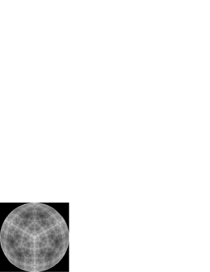
Figure 2: Quantum Tetrahedron. $\epsilon=0.5$ This is the simplest case.
The idea has been first described in [25] and then exploited in [27].

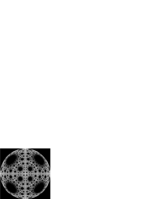
Figure 3: Quantum Octahedron. $\epsilon=0.58$

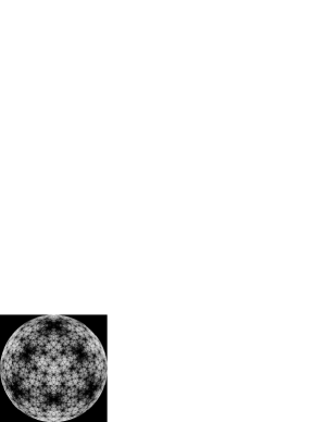
Figure 4: Quantum Cube. $\epsilon=0.7$

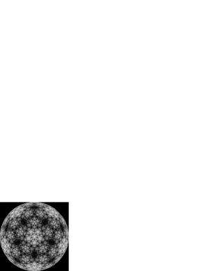
Figure 5: Quantum Icosahedron. $\epsilon=0.75$

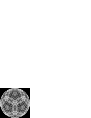
Figure 6: Quantum Dodecahedron. $\epsilon=0.78$

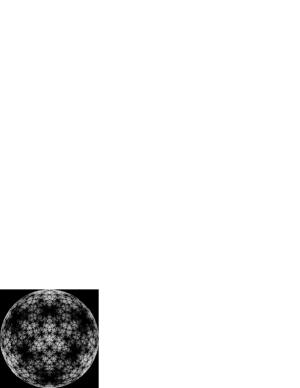
Figure 7: Quantum Double Tetrahedron. $\epsilon=0.7$

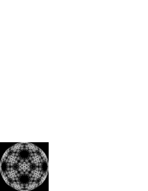
Figure 8: Quantum Icosidodecahedron. $\epsilon=0.85$

References

- [1] Carmichael H 1993 An open systems approach to quantum optics, Lecture Notes in Physics m 18, Springer Verlag, Berlin
- [2] Dalibard J, Castin Y and Mølmer K 1992 Wave–function approach to dissipative processes in quantum optics Phys. Rev. Lett. 68 580–3
- [3] Mølmer K, Castin Y and Dalibard J 1993 Monte Carlo wave–function method in quantum optics J. Opt. Soc. Am. B 10 524–38
- [4] Dum R, Zoller P and Ritsch H 1992 Monte Carlo simulation of the atomic master equation for spontaneous emission Phys. Rev. A 45 4879–87
-
[5]
Blanchard Ph and Jadczyk A, 1995
Event Enhanced Quantum Theory and Piecewise Deterministic
Dynamics Ann. der Physik 4 583–99 Preprint hep-th/9409189
(A review paper. Here a rough idea of the proof of the uniqueness of the PDP is sketched for the first time. The idea came from my discussions, in June and July 1994, with Heidi Narnhoffer at the Schrödinger Institute, Wien.) -
[6]
Blanchard Ph and Jadczyk A 1993 On the
interaction between classical and quantum systems Phys.
Lett. A 175 157-64
(The very first paper, describing the method of coupling of a quantum and of a classical system via dynamical semigroup. At that time we didn’t yet know about piecewise deterministic processes.) -
[7]
Blanchard Ph and Jadczyk A 1993 Strongly coupled
quantum and classical systems and Zeno’s effect Phys. Lett.
A 183 272–6 Preprint hep-th/9309112
(Here, for the first time, piecewise deterministic process describing individual systems is being mentioned. We wrote: ” To the Liouville equation describing the time evolution of statistical states of we will be in position to associate a piecewise deterministic process taking values in the set of pure states of . Knowing this process one can answer all kinds of questions about time correlations of the events as well as simulate the behaviour of individual quantum-classical systems. Let us emphasize that nothing more can be expected from a theory without introducing some explicit dynamics of hidden variables. What we achieved is the maximum of what can be achieved, which is more than orthodox interpretation gives. There are also no paradoxes; we cannot predict, but we can simulate the behaviour of individual systems.” At that time we didn’t yet know under what conditions our PDP is unique. That is why we used the term ”associated” with the Liouville equation, rather than ”derived”.) -
[8]
Jadczyk A 1995 Topics in Quantum Dynamics
Infinite Dimensional
Geometry, Noncommutative Geometry, Operator Algebras and
Fundamental Interactions ed R Coquereaux et al (Singapore World
Scientific) it Preprint hep-th/9406204
( A review paper. Describes the PDP process. States the problem: ”How to determine state of an individual quantum system?” Describes a process on which later was adapted for generation of quantum fractals.) -
[9]
Jadczyk A 1995 Particle Tracks, Events and Quantum
Theory Progr. Theor. Phys. 93 631–46 Preprint hep-th/9407157
(A model of particle tracks using a continuous medium of detectors. Gives GRW ”spontaneous localization” model as a particular case.) - [10] Blanchard Ph and Jadczyk A 1996 Relativistic Quantum Events Found. Phys 26 1669–81 Preprint quant-ph/9610028
-
[11]
Blanchard Ph and Jadczyk A 1999 EEQT a way out
of the quantum trap, in Open Systems and measurement in
Relativistic Quantum Theory ed Breuer H -P and Petruccione
F (Springer-Verlag) Preprint quant-ph/9812081
(A review paper. With FAQ on EEQT.) - [12] von Neumann John 1955 Mathematical Foundations of Quantum Mechanics (Princeton University Press)
-
[13]
Davis M H A 1984 Lectures on Stochastic
Control and Nonlinear Filtering, Tata Institute of Fundamental
Research (Berlin: Springer Verlag), Berlin 1984
(This is where we have learned for the first time about the use of piecewise deterministic processs (PDP)) - [14] Davis M H A 1993 Markov models and optimization, (London Chapman and Hall)
- [15] Ruschhaupt A 2002 A Relativistic Extension of Event-Enhanced Quantum Theory J. Phys. A: Math. Gen. 35 9227-43 Preprint quant-ph/0204079
- [16] Ruschhaupt A 2002 Relativistic Time-of-Arrival and Traversal Time J. Phys. A: Math. Gen. 35 10429-43 Preprint quant-ph/0207014
- [17] Peres A and Terno D R 2003 Quantum Information and Relativity Theory Preprint quant-ph/0212023
-
[18]
Barnsley M F 1988 Fractals everywhere (San
Diego: Academic Press)
(The main textbook reference on Iterated Function Systems.) - [19] Peitgen H O, Hartmut J and Saupe D 1992 Chaos and Fractals. New Frontiers of Science (New Yprk Springer)
- [20] Peigné Marc 1993 Iterated Function Systems and spectral decomposition of the associated Markov operator, Preprint U.R.A. C.N.R.S. 305
- [21] Casati G 1991 Quantum mechanics and chaos, in Chaos and Quantum Physics eds M. J. Gianoni, A. Voros and J. Zinn-Justin, (North Holland)
- [22] Casati G, Maspero G, and D. L. Shepelyansky 1999 Quantum fractal eigenstates Physica D 131 pp. 311-6 Preprint cond-mat/9710118
-
[23]
Jadczyk A, Kondrat G and Olkiewicz R 1996 On
uniqueness of the jump process in quantum measurement theory
J. Phys. A: Math. Gen. 30 1–18 Preprint quant-ph/9512002
// (A rigorous proof of the uniqueness theorem.) - [24] Information at the URL: http://www.cassiopaea.org/quantum_future/qfractals.htm
- [25] Jadczyk A 1993 IFS Signatures of Quantum States Preprint IFT Uni Wroclaw internal report
-
[26]
Blanchard Ph, Jadczyk A and Olkiewicz R 2001
Completely mixing quantum open systems and quantum fractals
Physica D 148 227-41 Preprint quant-ph/9909085
(Quantum fractals from simultaneous measurement of noncommuting observables.) - [27] Jastrzebski G. 1996 Interacting classical and quantum systems. Chaos from quantum measurements Ph.D. thesis, University of Wrocław (in Polish)
-
[28]
Blanchard Ph, Jadczyk A and Ruschhaupt A 2000 How Events
did come into beeing: EEQT, Particle Tracks, Quantum Chaos, and
Tunneling Time J. Mod. Opt. 47 2247–63 Preprint 9911113
(A review paper: particle tracks, GRW, Born’s interpretation, tunneling time, quantum fractals - the tetrahedron model.) - [29] Luminet J P, Weeks J, Riazuelo A, Lehoucq R, Uzan J P 2003 Dodecahedral space topology as an explanation for weak wide-angle temperature correlations in the cosmic microwave background Preprint astro-ph/0310253
- [30] Lozinski A, Zyczkowski K and Slomczynski W 2002 Quantum Iterated Function Systems Preprint quant-ph/0210029
- [31] Greub W, Halperin S and Vanstone B 1972 Connections, Curvature, and Cohomology, Vol I, Exercise 4 p 273 (New York: Academic Press)