Distilling Gaussian states with Gaussian operations is impossible

Abstract

We will show that no distillation protocol for Gaussian quantum states exists that relies on (i) arbitrary local unitary operations that preserve the Gaussian character of the state and (ii) homodyne detection together with classical communication and postprocessing by means of local Gaussian unitary operations on two symmetric identically prepared copies. This analysis shows that unlike the finite-dimensional case, where entanglement can be distilled in an iterative protocol using two copies at a time, there is no such procedure in the case of continuous variables for Gaussian initial states and the above Gaussian operations. The ramifications for the distribution of Gaussian states over large distances will be outlined. We will also comment on the generality of the approach and sketch the most general form of a Gaussian local operation with classical communication in a bi-partite setting.

In most practical implementations of information processing devices sophisticated methods are necessary in order to preserve the coherence of the involved quantum states. Even the mere preparation of an entangled state of spatially distributed quantum systems requires such techniques: once prepared locally and then distributed, an entangled state will to some extent deteriorate from a highly entangled state to a less correlated state through the process of decoherence. This process can quite obviously not be entirely avoided. However, one may prepare and distribute several identical entangled states, and then apply appropriate partly measuring local quantum operations and classical communication to obtain states that are similar to the highly entangled original state. This is only possible at the expense that one has fewer identically prepared systems or copies at hand, but this is a small price to pay. Appropriately indeed, this process has been given the name distillation [1], as fewer more highly entangled states are ’distilled’ from a supply of many less entangled states. It was one of the major successes of the field of quantum information science to realize that for two-level systems such a distillation procedure may be performed on only two copies at a time, and it requires only two steps: (i) a local unitary operation, and (ii) a local measurement, together with the classical communication about the measurement outcome. Based on the measurement outcome further local unitary operations are then implemented.

Such distillation protocols may also be of crucial importance in the infinite-dimensional setting. Quantum information science over continuous variables has seen an enormous progress recently, both in theory and experiment, mostly involving Gaussian states of field modes in a quantum optical setting [2, 3, 4]. Quite naturally, one should expect that a similar distillation procedure also works for Gaussian states in the infinite-dimensional case, also under the preservation of the Gaussian character of the state. If one transmits two pure two-mode squeezed Gaussian states through lossy optical systems such as fibers, the corresponding modes being from now on labeled $A1$, $A2$, $B1$, and $B2$, one obtains two identical copies of less entangled symmetric states [5]. A feasible distillation protocol preserving the Gaussian character may consist of the subsequent steps (see Fig. 1):

(i) Application of any local Gaussian unitary operation. That is, one may implement any unitary operations $U_{A}$ and $U_{B}$ on both $A1$ and $A2$ on one hand and $B1$ and $B2$ on the other hand corresponding to symplectic transformations [6] $S_{A},S_{B}\in Sp(4,{\mathbb{R}})$ [7]. This set includes all two-mode and one-mode squeezings, mixing at beam splitters and phase shifts. To specify these operations 20 real parameters are necessary. Note that we do not require both parties to realize the same transformation.

(ii) A homodyne measurement on the modes $A2$ and $B2$. The parties communicate classically about the outcome of the measurement, and may postprocess the states of modes $A1$ and $B1$ with unitary Gaussian operations.

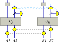
FIG. 1.: The class of considered feasible distillation protocols.

The main result of this Letter is that very much as a surprise, none of these protocols amounts to a distillation protocol. No matter how ingeniusely the local unitary operation is chosen, the degree of entanglement can not be increased. The optimal procedure is simply to do nothing at all, which means that at least no entanglement is lost [8]. The degree of entanglement will be measured in terms of the log-negativity, which is defined as $E_{N}(\rho)=\log_{2}\|\rho^{T_{A}}\|$ for a state $\rho$, where $\|.\|$ denotes the trace norm, and $\rho^{T_{A}}$ is the partial transpose of $\rho$. The negativity has been shown to be an entanglement measure in the sense that it is non-increasing on average under local operations with classical communication [9], and is to date the only known feasible measure of entanglement for Gaussian states. For pure (and for symmetric mixed) Gaussian states it is related to the degree of squeezing in a monotone way (see, e.g., [10]). This means that as a corollary of the main result, it follows that with Gaussian operations as specified above one cannot transform two identically prepared two-mode squeezed vacua into a single two-mode squeezed vacuum state with a higher degree of squeezing.

We will start by fixing the notation. Gaussian states [11] of an $n$-mode system are completely characterized by their first and second moments. The first moments are the expectation values of the canonical coordinates. The second moments can be collected in the real symmetric covariance matrix $\Gamma\!\in\!C(2n)\!\subset\!M({2n},{\mathbb{R}})$, where $M({2n},{\mathbb{R}})$ denotes the set of real $2n\times 2n$-matrices, and $C(2n)$ the subset of matrices obeying the Heisenberg uncertainty principle [11]. The linear transformations from one set of canonical coordinates to another which preserve the canonical commutation relations form the group of real linear symplectic transformations $Sp(2n,\mathbb{R})$ [6]. A symplectic transformation $S$ changes the covariance matrix according to $\Gamma\longmapsto S\Gamma S^{T}$, while states undergo a unitary operation $\rho\longmapsto U\rho U^{\dagger}$. The $n\!=\!4$ modes $A1$, $A2$, $B1$, $B2$ will be equipped with the canonical operators $(X_{A1},P_{A1},...,X_{B2},P_{B2})$. To make the notation more transparent, both tensor products and direct sums will carry a label indicating the underlying split, meaning either $A,B$ or $1,2$. We state the main result of this Letter in form of a theorem:

Theorem. – Let $\rho\otimes\rho$ be two identically prepared symmetric Gaussian states of two-mode systems consisting of the parts $A1$, $A2$, $B1$, and $B2$, respectively, each of which having the covariance matrix

$$\Gamma^{{(0)}}=\left(\begin{array}[]{cccc}a&0&c&0\\ 0&a&0&-c\\ c&0&a&0\\ 0&-c&0&a\\ \end{array}\right),\,\,a\geq 1,\,\,0\leq c\leq(a^{2}-1)^{1/2},$$ (1)

let $S_{A},S_{B}\in Sp(4,{\mathbb{R}})$ be any symplectic transformations with associated unitaries $U_{A}$ and $U_{B}$, and let

$$\rho^{\prime}=(U_{A}\otimes_{A,B}U_{B})(\rho\otimes_{1,2}\rho)(U_{A}\otimes_{A,B}U_{B})^{\dagger}.$$ (2)

Then any state $\rho^{\prime\prime}$ that is obtained from $\rho^{\prime}$ via a selective homodyne measurement on systems $A2$ and $B2$ satisfies $E_{N}(\rho^{\prime\prime})\leq E_{N}(\rho)$, that is, the degree of entanglement can only decrease.

The proof of this statement will turn out to be technically involved, and while the statement itself is concerned with practical quantum optics, the techniques used in the proof will be mostly taken from matrix analysis [12]. In order to give the general argument more structure, the proof is split into several lemmata. The entire proof will be formulated in terms of covariance matrices, rather than in terms of the states.

The log-negativity of a state $\sigma$ of a two-mode system can be easily expressed in terms of the entries of the associated covariance matrix $\gamma\in C(4)$. The latter can be partitioned in block form according to

$$\gamma=\left(\begin{array}[]{cc}\gamma_{A}&\gamma_{C}\\ \gamma_{C}^{T}&\gamma_{B}\\ \end{array}\right),\,\,\,\gamma_{A},\gamma_{B},\gamma_{C}\in M(2,R).$$ (3)

The log-negativity $E_{N}(\sigma)$ is then given by [9]

$$E_{N}(\sigma)=\left\{\begin{array}[]{cc}-(\log\circ f)(\gamma)/2,&\text{if }f(\gamma)<1,\\ 0&\text{otherwise.}\end{array}\right.$$ (6)

where the function $f:C(4)\longrightarrow{\mathbb{R}}^{+}$ is defined as

$$f(\gamma) = ((\text{det}[\gamma_{A}]+\text{det}[\gamma_{B}])/2-\text{det}[\gamma_{C}])$$ (7)

$$- \bigl{[}((\text{det}[\gamma_{A}]+\text{det}[\gamma_{B}])/2-\text{det}[\gamma_{C}])^{2}-\text{det}[\gamma]\bigr{]}^{1/2}.$$ (8)

The covariance matrix associated with the Gaussian state $\rho^{\prime}$ in the Theorem will be denoted as $\Gamma^{\prime}\in C(8)$. For any $S_{A},S_{B}\in Sp(4,{\mathbb{R}})$ this covariance matrix of the modes $A1$, $A2$, $B1$, and $B2$ becomes $\Gamma^{\prime}:=(S_{A}\oplus_{A,B}S_{B})(\Gamma^{(0)}\oplus_{1,2}\Gamma^{(0)})(S_{A}\oplus_{A,B}S_{B})^{T}$ The first step is to relate the covariance matrix $\Gamma^{\prime\prime}$ associated with the state after the measurement to a Schur complement [12]. This Schur complement structure is a general feature of Gaussian operations and will be further discussed at the end of the letter.

Lemma 1. – Let $\Gamma^{\prime}\in C(8)$ be a covariance matrix of systems $A1$, $A2$, $B1$, and $B2$ associated with a state $\rho^{\prime}$, which can be written in block form as

$$\Gamma^{\prime}=\left(\begin{array}[]{cc}C_{1}&C_{3}\\ C_{3}^{T}&C_{2}\\ \end{array}\right),$$ (9)

where $C_{1},C_{2},C_{3}\in M(4,{\mathbb{R}})$. The covariance matrix of the state that is obtained by a projection in $A2$ and $B2$ on the pure Gaussian state with covariance matrix $D_{d}:=\text{diag}(1/d,d,1/d,d)\in C(4)$, $d>0$, is then given by

$$M_{d}=C_{1}-C_{3}(C_{2}+D_{d}^{2})^{-1}C_{3}^{T}.$$ (10)

Proof. This statement can be most conveniently be shown in terms of the characteristic function $\chi$ [11]. By employing the Weyl (displacement) operator, the state $\rho^{\prime}$ associated with the covariance matrix $\Gamma^{\prime}$ can be written in terms of the characteristic function according to $\rho^{\prime}=(1/\pi^{4})\int d^{8}\xi\,W(-\xi)\chi(\xi)$ (see, e.g., Ref. [13]). The projection corresponds on the level of the characteristic function therefore to an incomplete Gaussian integration. The characteristic function associated with the modes $A1$ and $B1$ can then be written as

$$\chi(\xi_{1},\dots,\xi_{4}) = \int\frac{d\xi_{5}\dots d\xi_{8}}{\pi^{2}}e^{-\xi^{T}\Gamma^{\prime}\xi/2}e^{-\frac{1}{2d^{2}}(\xi_{5}^{2}+\xi_{7}^{2})-\frac{d^{2}}{2}(\xi_{6}^{2}+\xi_{8}^{2})}$$ (11)

$$= |C_{2}+D_{d}^{2}|^{-1/2}e^{-(\xi_{1},\dots,\xi_{4})\Gamma^{\prime\prime}(\xi_{1},\dots,\xi_{4})^{T}/2},$$ (12)

with $M_{d}$ defined as in Eq. (10).  

Hence, the resulting covariance matrix is given by the Schur complement $C_{1}-C_{3}(C_{2}+D_{d}^{2})^{-1}C_{3}^{T}$ of the matrix

$$\Gamma_{d}^{\prime}:=\left(\begin{array}[]{cc}C_{1}&C_{3}\\ C_{3}^{T}&C_{2}+D_{d}^{2}\\ \end{array}\right)$$ (13)

with respect to the leading principal submatrix $C_{1}$. The additional matrix $D_{d}^{2}$ originates from the projection in the modes $A2$ and $B2$. Note that although this Lemma has been formulated in terms of the projection on a certain class of pure Gaussian states, it applies to the projection on any pure Gaussian state in the modes $A2$ and $B2$: the projection on any other pure Gaussian state can be realized by an appropriate choice of the symplectic transformations $S_{A}$ and $S_{B}$. Ideal homodyne detections can now be formulated as projections on ‘infinitely squeezed’ pure Gaussian states [13]. The central feature is that the initial first moments do not affect the form of the covariance matrix after the measurement. Lemma 2 gives the form of the resulting covariance matrix in case of a homodyne detection in modes $A2$ and $B2$. In the limit $d\rightarrow 0$ the matrix $D_{d}$ gives rise to a projection operator, and the inverse becomes a Moore Penrose inverse (MP) [12]:

Lemma 2. – In the notation of Lemma 1, the covariance matrix of modes $A1$ and $B1$ after a selective homodyne measurement in modes $A2$ and $B2$ is given by

$$\Gamma^{\prime\prime}:=\lim_{d\rightarrow 0}\Gamma_{d}=C_{1}-C_{3}(\pi C_{2}\pi)^{\text{MP}}C_{3}^{T},$$ (14)

where $\pi=\text{diag}(1,0,1,0)$.

Equipped with these preparatory considerations, we will now turn to the core of the proof. In order to be able to evaluate the logarithmic negativity according to Eq. (6), one needs to know the values of the invariants under local symplectic transformations, i.e., the determinants of four submatrices. To find an expression for all these determinants is however a quite difficult task. Instead, we will later make use of an upper bound of the logarithmic negativity that only involves determinants of principal submatrices [12] of $\Gamma^{\prime\prime}$.

Lemma 3. – Let $\Gamma^{\prime\prime}\in C(4)$ be defined as in Lemma 2. Then, independent of $S_{A},S_{B}\in Sp(4,{\mathbbm{R}})$,

$$\text{det}[\Gamma^{\prime\prime}]=\text{det}[\Gamma^{(0)}]=(a^{2}-c^{2})^{2}.$$ (15)

Proof. According to Lemma 2, $\Gamma^{\prime\prime}$ is given by $\Gamma^{\prime\prime}=\lim_{d\rightarrow 0}M_{d}$. The Schur complement of the matrix $\Gamma^{\prime}_{d}$ as defined in Eq. (13) is related to $\Gamma^{\prime}_{d}$ and one of its principal submatrices via the congruence

$$\left(\begin{array}[]{cc}\openone_{4}&X\\ 0&\openone_{4}\end{array}\right)\Gamma^{\prime}_{d}\left(\begin{array}[]{cc}\openone_{4}&0\\ X^{T}&\openone_{4}\end{array}\right)=\left(\begin{array}[]{cc}\Gamma_{d}&0\\ 0&C_{2}+D_{d}^{2}\end{array}\right),$$ (16)

where $X:=-C_{3}(C_{2}+D_{d}^{2})^{-1}$. Hence, according to the determinant multiplication theorem we obtain $\text{det}[\Gamma^{\prime}_{d}]=\text{det}[\Gamma_{d}]\,\text{det}[C_{2}+D_{d}^{2}]$, which yields in the limit $d\rightarrow 0$

$$\text{det}[\Gamma^{\prime\prime}]=\text{det}[P\Gamma^{\prime}_{d}P+(\openone_{8}-P)]/\text{det}[Q\Gamma^{\prime}_{d}Q+(\openone_{8}-Q)],$$ (17)

where the projections $P$ and $Q$ are defined as $P:=\text{diag}(1,1,1,1,0,1,0,1)$ and $Q:=\text{diag}(0,0,0,0,0,1,0,1)$. With these tools, it is feasible to directly prove the statement of Lemma 3 by parameterizing $S_{A},S_{B}\in Sp(4,{\mathbbm{R}})$. Every $S\in Sp(4,{\mathbbm{R}})$ can be written as a product $S=VDW$, where $V,W\in Sp(4,{\mathbbm{R}})\cap SO(4)$, and $D:=\text{diag}(d_{1},1/d_{1},d_{2},1/d_{2})$ with $d_{1},d_{2}\in{\mathbbm{R}}$ [6].  

Lemma 4. – Let $\Gamma^{\prime\prime}\in C(4)$ be defined as in Lemma 2, and let $\Gamma_{A}^{\prime\prime}$ and $\Gamma_{B}^{\prime\prime}$ be the principal submatrices belonging to mode $A1$ and $B1$. Then, for all $S_{A},S_{B}\in Sp(4,{\mathbbm{R}})$,

$$\text{det}[\Gamma_{A}^{\prime\prime}]\leq\text{det}[\Gamma^{(0)}_{A}]=a^{2},\,\,\text{det}[\Gamma_{B}^{\prime\prime}]\leq\text{det}[\Gamma^{(0)}_{B}]=a^{2}.$$ (18)

Proof. ${\Gamma^{\prime\prime}}$ is defined as the covariance matrix corresponding to modes $A1$ and $B1$ after the projective measurements in both $A2$ and $B2$. Let us assume that one first performs the projective measurement in $A2$, leading to a the covariance matrix $N_{A}\in C(2)$ of the reduced state of $A1$. The covariance matrix $\Gamma_{A}^{\prime\prime}$ after the projection in $B2$ is then obtained as a Schur complement. In particular, $\Gamma_{A}^{\prime\prime}$ can be written as $\Gamma_{A}^{\prime\prime}=N_{A}-R$, where $R\in M(2,{\mathbbm{R}})$ is a real symmetric positive matrix. Hence, as $\Gamma_{A}^{\prime\prime}$ and $N_{A}$ are also positive, $\text{det}[\Gamma_{A}^{\prime\prime}]\leq\text{det}[N_{A}]$ [12]. In other words, one obtains an upper bound for $\text{det}[\Gamma_{A}^{\prime\prime}]$ when considering only a projective measurement in $A1$. The statement of Lemma 4 follows from Lemma 3 in the special case that $c=0$: one can after a few steps conclude that then $\text{det}[N_{A}]=a^{2}$, independent of $S_{A},S_{B}\in Sp(4,{\mathbbm{R}})$. The same reasoning applies to $\Gamma_{B}^{\prime\prime}$.  

The most important step is now an appropriate upper bound of the log-negativity of the resulting state. The actual bound might appear somewhat arbitrary, but it will turn out that it is exactly the tool that we need in the last step of the proof.

Lemma 5. – Let $\gamma\in C(4)$, partitioned as in Eq. (3). Then

$$f(\gamma)\geq g(\gamma) := \bigl{[}\left((\text{det}[\gamma_{A}]+\text{det}[\gamma_{B}])/2\right)^{1/2}$$ (19)

$$- ((\text{det}[\gamma_{A}]+\text{det}[\gamma_{B}])/2-\text{det}[\gamma]^{1/2})^{1/2}\bigr{]}^{2}.$$ (20)

Proof. $g(\gamma)$ can be expressed in terms of $f$ as $g(\gamma)=f(\gamma^{\prime})$,

$$\gamma^{\prime}=\left(\begin{array}[]{cc}\gamma_{A}^{\prime}&\gamma_{C}^{\prime}\\ {\gamma_{C}^{\prime}}^{T}&\gamma_{B}^{\prime}\end{array}\right),\,\,\,\gamma^{\prime}_{A}=\gamma^{\prime}_{B}=a^{\prime}\openone_{2},\,\,\,\gamma^{\prime}_{C}=\left(\begin{array}[]{cc}c^{\prime}&0\\ 0&-c^{\prime}\\ \end{array}\right),$$ (21)

where $a^{\prime}:=((\text{det}[\gamma_{A}]^{2}+\text{det}[\gamma_{B}]^{2})/2)^{1/2}$ and $c^{\prime}:=({a^{\prime}}^{2}-\text{det}[\gamma]^{1/2})^{1/2}$. Hence, one has to prove that $f(\gamma^{\prime})\leq f(\gamma)$. Firstly, note that $\text{det}[\gamma]=\text{det}[\gamma^{\prime}]$. Secondly, $(\text{det}[\gamma_{A}]+\text{det}[\gamma_{B}])/2={a^{\prime}}^{2}$. Therefore, it remains to be shown that ${c^{\prime}}^{2}\geq|\text{det}[\gamma_{C}]|$. This inequality is equivalent with $\left[(\text{det}[\gamma_{A}]+\text{det}[\gamma_{B}])/2-|\text{det}[\gamma_{C}]\,|\right]^{2}-\text{det}[\gamma]\geq 0$, which is a valid inequality, as $\gamma\in C(4)$.  

Proof of the Theorem. Let ${\Gamma^{\prime\prime}}\in C(4)$ be the matrix defined as in Lemma 2. The log-negativity of the corresponding state of modes $A1$ and $B1$ is given by $-(\log\circ f)({\Gamma^{\prime\prime}})$, if the final state is entangled at all, as we will assume from now on. Lemma 5 yields the bound $f({\Gamma^{\prime\prime}})\geq g({\Gamma^{\prime\prime}})$. In $g({\Gamma^{\prime\prime}})$, however, only the determinants of the principal submatrices are needed, bounds of which are available by virtue of Lemma 3 and 4. The function $h:[y,\infty)\rightarrow{\mathbbm{R}}^{+}$ with $h(x)=(x^{1/2}-(x-y)^{1/2})^{2}$, $y>0$, is a strictly monotone decreasing function of $x$. Therefore, using Lemma 3 and 4 one can conclude that $g({\Gamma^{\prime\prime}})\geq g(\Gamma^{(0)})$. Moreover, $g(\Gamma^{(0)})=f(\Gamma^{(0)})$, due to the special form of $\Gamma^{(0)}$, as can be easily verified. Hence, $f({\Gamma^{\prime\prime}})\geq g(\Gamma^{(0)})=f(\Gamma^{(0)})$, which leads to $-(\log\circ f)({\Gamma^{\prime\prime}})\leq-(\log\circ f)(\Gamma^{(0)})$. This is finally the desired result: it means that the degree of entanglement can only decrease.  

We will finally comment on the generality of the approach. A general Gaussian operation is a quantum operation that maps all Gaussian states on Gaussian states [3]. Any general Gaussian local operation with classical communication (LOCCG) – trace-preserving or non-trace-preserving – can be decomposed into the subsequent steps: (i) Appending locally additional modes that have been prepared in a Gaussian state [3]. (ii) Application of any local unitary Gaussian operation on both the original and the additional system. These comprise operations corresponding to symplectic transformations and displacements in phase space. (iii) Projections on pure Gaussian states or ideal homodyne detections, which give rise to Schur complements on the level of covariance matrices as described above, together with the classical communication about the outcome (real numbers in case of homodyne detection, bits in case of dichotomic measurements including the projection on a pure Gaussian state in one outcome), (iv) mixing, such that the resulting state is Gaussian, and (v) a partial trace, which corresponds to considering a certain principal submatrix of the covariance matrix only [14]. The proof is therefore restrictive in the sense that only two copies at a time are considered, other projections on Gaussian states are excluded, and no additional modes are allowed for. The statement of the present paper proves that iterative protocols in strict analogy to the corresponding methods in finite dimensional settings certainly do not work. Indeed, the findings strongly suggest that Gaussian states cannot be distilled at all with Gaussian operations. Then (less feasible) non-linear physical effects [15] would have to be made use of in order to distill from a supply of Gaussian two-mode states [16]. Such techniques would then also be necessary for the realistic implementation of quantum repeaters [17] for continuous-variable systems when it comes to the distribution of highly entangled Gaussian states over large distances.

We would like to thank K. Audenaert, J. Fiurášek, P. van Loock, C. Silberhorn, G. Giedke, J.I. Cirac, S.D. Bartlett, B.C. Sanders, D.-G. Welsch, and N.  Cerf for discussions. This work has been supported by the European Union (EQUIP, QUEST) and the A.-v.-Humboldt-Foundation.

REFERENCES

- [1] C.H. Bennett, G. Brassard, S. Popescu, B. Schumacher, J.A. Smolin, W.K. Wootters, Phys. Rev. Lett. 76, 722 (1996); D. Deutsch, A. Ekert, R. Jozsa, C. Macchiavello, S. Popescu, and A. Sanpera, ibid. 77, 2818 (1996).
- [2] S. Lloyd and S.L. Braunstein, Phys. Rev. Lett. 82, 1784 (1999); R. Simon, ibid. 84, 2726 (2000); J. Fiurášek, ibid. 86, 4942 (2001); L.-M. Duan, G. Giedke, J.I. Cirac, and P. Zoller, ibid. 84, 2722 (2000); G. Lindblad, J. Phys. A 33, 5059 (2000); N.J. Cerf and S. Iblisdir, Phys. Rev. A 62, 040301 (2000); S. Parker, S. Bose, and M.B. Plenio, Phys. Rev. A 61, 032305 (2000); P. van Loock and S.L. Braunstein, ibid. 63, 022106 (2001); J. Eisert, C. Simon, and M.B. Plenio, J. Phys. A 35, 3911 (2002); S.L. Braunstein and H.J. Kimble, Phys. Rev. Lett. 80, 869 (1998); C. Silberhorn, P.K. Lam, O. Weiss, F. König, N. Korolkova, G. Leuchs, ibid. 86, 4267 (2001).
- [3] J. Eisert and M.B. Plenio, Phys. Rev. Lett. 89, 097901 (2002); J. Fiurášek, quant-ph/0202102; B. Demoen, P. Vanheuverzwijn, and A. Verbeure, Lett. Math. Phys. 2, 161 (1977).
- [4] G. Giedke, L.-M. Duan, J.I. Cirac, and P. Zoller, Quant. Inf. Comp. 1, 79 (2001).
- [5] S. Scheel, L. Knöll, T. Opatrný, and D.-G. Welsch, Phys. Rev. A 62, 043803 (2000); D.-G. Welsch, S. Scheel, and A.V. Chizhov, quant-ph/0105111.
- [6] R. Simon, E.C.G. Sudarshan, and N. Mukunda, Phys. Rev. A 36, 3868 (1987); R. Simon, N. Mukunda and B. Dutta, ibid. 49 1567 (1994); Arvind et al., quant-ph/9509002.
- [7] Both parties may also apply displacements in phase space, which can always be implemented locally.
- [8] In contrast, it has been shown that from any bi-partite Gaussian state with a non-positive partial transpose singlets can be distilled in principle using general quantum operations (obviously under loss of the Gaussian character of the state) [4].
- [9] J. Eisert, PhD thesis (Potsdam, February 2001); G. Vidal and R.F. Werner, Phys. Rev. A 65, 032314 (2002).
- [10] M.M. Wolf, J. Eisert, and M.B. Plenio, quant-ph/0206171.
- [11] In terms of the canonical coordinates the entries of the covariance matrix are given by , , where the skew-symmetric -matrix is defined as . Any symmetric matrix satisfying the Heisenberg uncertainty principle is a covariance matrix. The defining property of Gaussian states is that their characteristic function is a Gaussian function in phase space, where denotes the Weyl operator. The Wigner function, as often employed in this context, is given by the Fourier transform of the characteristic function.
- [12] R.A. Horn and C.R. Johnson, Matrix Analysis (Cambridge University Press, Cambridge, 1985).
- [13] W. Vogel, D.-G. Welsch, and S. Wallentowitz, Quantum Optics, An Introduction (Wiley-VCH, Berlin, 2001).
- [14] Note that Gaussian operations including projections on pure Gaussian states can also be implemented by means of symplectic transformations and homodyne measurements.
- [15] Compare also [S.D. Bartlett, B.C. Sanders, S.L. Braunstein, and K. Nemoto, Phys. Rev. Lett. 88, 097904 (2002)].
- [16] J. Clausen, L. Knöll, and D.-G. Welsch, quant-ph/0203144.
- [17] H.-J. Briegel, W. Dür, J.I. Cirac, and P. Zoller, Phys. Rev. Lett. 81, 5932 (1998).