Quantum limits on phase-shift detection using multimode interferometers

Abstract

Fundamental phase-shift detection properties of optical multimode interferometers are analyzed. Limits on perfectly distinguishable phase shifts are derived for general quantum states of a given average energy. In contrast to earlier work, the limits are found to be independent of the number of interfering modes. However, the reported bounds are consistent with the Heisenberg limit. A short discussion on the concept of well-defined relative phase is also included.

PACS numbers: 42.50.-p, 03.65.Ta, 07.60.Ly, 42.50.Dv

I Introduction

It is today well-known that the use of quantum-mechanical states can improve the precision of interferometric measurements. According to the so-called standard quantum limit [1], the precision of optical measurements employing classical states cannot increase faster than $\propto 1/\sqrt{E}$, where $E$ is the energy used in the measurement. However, the use of nonclassical states allows us to reach the Heisenberg limit $\propto 1/E$ [2], which for high energies would give a remarkable improvement in accuracy. Several setups have theoretically been shown to work at the Heisenberg limit [3, 4, 5, 6]. The standard quantum limit has also been circumvented experimentally [7, 8, 9, 10]. However, the fragile nature of the quantum states has so far prevented these measurements from being carried out with higher energies. Therefore, high intensity classical interferometry reach a much better overall accuracy.

Recently, a bound closely related to the Heisenberg limit was given by Margolus and Levitin [11]. The bound gives the time necessary for a state of a closed system to become orthogonal for a given average energy. This limits the rate of operations in quantum information processing and the resolution in interferometry. In an earlier paper [12], we derived the states that minimize the time needed to freely evolve into another state, whose overlap with the original one was given. This would correspond to minimizing the necessary phase shift for a single-mode state.

The present paper is devoted to the phase-shift detection properties of multimode interferometers. In many interferometric measurements, a single induced phase shift is tracked by monitoring the interference fringes in the output of a two-mode interferometer. However, it is often possible to induce several phase shifts of the same, or smaller, magnitude (possibly with different signs) in the different arms of a multimode interferometer. Here, we investigate whether this fact can be used to improve the accuracy of such measurements. We will assume that the interfering fields have the same optical frequency, so that the total energy is proportional to the number of photons used.

In an earlier investigation [13], it was concluded that the accuracy of the multimode interferometer would improve indefinitely with the number of modes. However, we find that there is no fundamental advantage in using more than two modes and that, in our eyes, the conclusions in Ref. [13] stem from an unfortunate choice of figure of merit. Rather, the accuracy is found to be limited only by the energy used in the measurement and scale according to the Heisenberg limit.

II Problem formulation

Accuracy can be defined in many different ways. For example, in a recent paper on multimode interferometry [14], the width of the major peak of the phase distribution was taken as a measure of the precision. Here, we will define it as the smallest phase shift required to give a perfectly distinguishable outcome, i.e., the phase-shifted state is required to be orthogonal to the original state.

More precisely, we look for the smallest phase shift that can be detected with certainty using an $M$-mode interferometer and a state whose average energy is given. The smallest phase shift $\phi$ should here be interpreted in the following sense (cf. Figs. 1 and 2). We consider the case where all arms of the interferometer have induced phase shifts that satisfy $\phi_{m}=\lambda_{m}\phi$, where $-1\leq\lambda_{m}\leq 1$ and $\phi>0$ is the parameter to be minimized under the condition that it results in a state that is perfectly distinguishable from the original. Since the $N$-photon state $(|0,N\rangle+|N,0\rangle)/\sqrt{2}$ can be made orthogonal in a two-mode interferometer by a relative phase shift of $\pi/N$ [5], and the two-mode interferometer is a special case of the multimode interferometer considered here, we know that the smallest necessary phase shift $\phi$ is smaller than, or equal to, $\pi/2N$.

Minimizing $\phi$ above corresponds to an experimental situation where we have an arbitrary number of induced phase shifts at our disposal (one in each mode). However, we easily identify another experimental situation of interest, where we have a given amount of phase shift that can be split and distributed among the modes. If we are also allowed to choose the signs of the phase shifts, our problem is to minimize $\phi_{\rm tot}=\sum_{m=1}^{M}|\phi_{m}|$. We will see that the solution to this problem also gives a tight bound for the case where all phase shifts have the same sign.

In accordance with our discussion above, we consider an $M$-mode interferometer with phase shifts $\phi_{m}=\lambda_{m}\phi$, where $-1\leq\lambda_{m}\leq 1$, in the different arms. We will also, without any loss of generality, number the modes in such a way that $\lambda_{1}\geq\lambda_{2}\geq\ldots\geq\lambda_{M}$. The two problems formulated above can then be expressed in a mathematical form as follows: We want to find the smallest value of $\phi$ and $\phi_{\rm tot}=\sum_{m=1}^{M}|\phi_{m}|$, respectively, such that

$$\langle\Psi|e^{i\phi\sum_{m=1}^{M}\lambda_{m}\hat{n}_{m}}|\Psi\rangle=0,$$ (1)

for some pure $M$-mode state $|\Psi\rangle$ with a given average energy. In particular, we are, in correspondence with the Heisenberg limit, looking for the minimum product of our accuracy measure ($\phi$ or $\phi_{\rm tot}$) and the average photon number $\langle\hat{N}\rangle$.

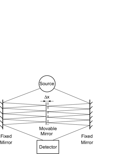
FIG. 1.: A sketch of an interferometric setup to probe the displacement $\Delta x$ of the two-sided mirror at the center. As the movable mirror is displaced by $\Delta x$ to the right, the phase shift in the left mode becomes $\phi_{\rm left}=2\pi R_{\rm left}\Delta x/\lambda_{0}\cos\gamma$, where $R_{\rm left}$ is the number of times the beam runs between the left and center mirror, $\lambda_{0}$ is the optical wavelength, $\gamma$ is the angle of incidence, and we have assumed unit refractive index. The phase shift in the right mode is given by a similar expression, but has opposite sign. In practice, the induced phase shift is always limited, e.g., due to the quality of the light beam. However, note that we, in principle, can use as many modes on each side of the movable mirror as we like. By an appropriate choice of the number of reflections and the angle of incidence for mode $m$, we can realize any phase shift satisfying $|\phi_{m}|\leq\phi$, where $\phi$ is the greatest possible phase shift for a single mode.

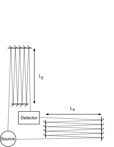
FIG. 2.: A generalized delay-line Michelson interferometer for detection of gravitational waves. As the $x$- and $y$-arm are perpendicular, quadrupole gravitational waves would, under certain conditions, induce changes in the mirror separations $L_{x}$ and $L_{y}$ that are of the same magnitude but with different signs [15]. The present setup then becomes equivalent to the one sketched in Fig. 1. Note that we consider a general source and detector, whereas the conventional delay-line Michelson interferometer used for gravitational wave detection consists of a laser source, a beam splitter and a photodetector.

III The energy eigenstates

In this section, we restrict ourself to the $N$-photon states. We derive lower bounds on $\phi$ and $\phi_{\rm tot}$, and give examples that saturate these bounds. The general case, where the states are allowed to be superpositions of different photon number states, is considered in Sec. IV.

A Minimizing $\phi$ with respect to N

Let $|\Psi_{N}\rangle$ denote a pure $M$-mode, $N$-photon state and introduce the nonnegative parameters $\mu_{m}=\lambda_{m}-\lambda_{M}$. The orthogonality condition (1) then becomes

$$\langle\Psi_{N}|e^{i\phi\sum_{m=1}^{M}\mu_{m}\hat{n}_{m}}|\Psi_{N}\rangle=0,$$ (2)

where $0\leq\mu_{m}\leq 2$ and $\mu_{1}\geq\mu_{2}\geq\ldots\geq\mu_{M}=0$. Furthermore, let $\{|{\cal N}_{j}^{(N)}\rangle\}_{j=1}^{J_{N}}$ denote the set of all possible orthogonal states

$$|{\cal N}_{j}^{(N)}\rangle=|n_{1,j}^{(N)},n_{2,j}^{(N)},\ldots,n_{M,j}^{(N)}\rangle$$ (3)

that for each $j$ fulfill

$$\sum_{m=1}^{M}n_{m,j}^{(N)}=N,\quad\quad n_{m,j}^{(N)}\in\{0,1,2,\ldots,N\}.$$ (4)

(The superscripts are not necessary here, but will be used in the next section.) A general pure $N$-photon state can then be written

$$|\Psi_{N}\rangle=\sum_{j=1}^{J_{N}}c_{j}^{(N)}|{\cal N}_{j}^{(N)}\rangle,$$ (5)

where $\sum_{j=1}^{J_{N}}|c_{j}^{(N)}|^{2}=1$. Putting this into Eq. (2) gives

$$\sum_{j=1}^{J_{N}}\left|c_{j}^{(N)}\right|^{2}\cos\left(\phi\sum_{m=1}^{M}\mu_{m}n_{m,j}^{(N)}\right)$$ (7)

$$+i\sum_{j=1}^{J_{N}}\left|c_{j}^{(N)}\right|^{2}\sin\left(\phi\sum_{m=1}^{M}\mu_{m}n_{m,j}^{(N)}\right)=0.$$

In order for the imaginary part to vanish, the smallest definite phase shift we can use is $\phi=\pi/2N$, which implies that $c_{j}^{(N)}=0$, for all $j$ such that $\sum_{m=1}^{M}\mu_{m}n_{m,j}^{(N)}\neq 0$ or $2N$. We must also have $\mu_{1}=2$ (remember that the parameters are labeled in decreasing order). Now, let $p_{0}$ denote the sum of $|c_{j}^{(N)}|^{2}$ over all $j$ such that $\sum_{m=1}^{M}\mu_{m}n_{m,j}^{(N)}=0$. The condition for the real part to vanish then becomes $p_{0}-(1-p_{0})=0$, i.e., $p_{0}=1/2$. The simplest state that fulfills this has only two nonzero coefficients $c_{j}^{(N)}$. An example of such a state is

$$|\Phi_{N}\rangle=\frac{1}{\sqrt{2}}\left(|N,0,\ldots,0\rangle+e^{i\vartheta}|0,0,\ldots,N\rangle\right),$$ (8)

where $\vartheta$ is an arbitrary real number. This state makes it possible to detect a phase shift of $\pi/2N$ with certainty. As shown above, this is the smallest phase shift that can be detected with certainty using $N$-photon states. We also note that the state (8) can be seen as a representation of a two-mode interferometer, since all but two modes (arms) are left unexcited. That is, the resolution limit $\phi=\pi/2N$ can be reached with a two-mode interferometer.

B Minimizing $\phi_{\rm tot}$ with respect to N

Now, assume that $|\Psi_{N}\rangle$ is an $N$-photon state that together with the phase shifts $\phi_{m}=\lambda_{m}\phi$ minimize $\phi_{\rm tot}=\sum_{m=1}^{M}|\phi_{m}|$ under the condition (1). Equation (1) then implies that Eqs. (2) and (7) are satisfied, where $\mu_{m}\phi=\phi_{m}-\phi_{M}$. Since the real part of the expression (7) must vanish, we have $\phi\sum_{m=1}^{M}\mu_{m}n_{m,j}^{(N)}>0$, for some $j$. In order for the imaginary part to vanish, it then follows that $\phi\sum_{m=1}^{M}\mu_{m}n_{m,j}^{(N)}\geq\pi$, for some $j$. Thus, there exists an $m$ such that $\phi_{m}-\phi_{M}\geq\pi/N$, i.e., $\phi_{\rm tot}\geq\pi/N$. This bound, too, can be saturated by the state (8), if we choose $\phi_{1}=\pi/2N$ and $\phi_{M}=-\pi/2N$. Again, we find that the lower bound can be achieved with a two-mode interferometer.

C The de Broglie wavelength

Note that the bounds we have obtained for the $N$-photon states are easily interpreted in terms of their de Broglie wavelength $\lambda_{\rm dB}=\lambda_{0}/N$, where $\lambda_{0}$ is the optical wavelength [5]. We know that an ordinary two-mode interferometer fed with classical light (or a single photon) needs a relative phase shift of $\pi$, corresponding to half the optical wavelength, in order to change between constructive and destructive interference. If we instead feed the interferometer with nonclassical states of light with an average energy $\langle\hat{N}\rangle$, the corresponding de Broglie wavelength is limited from below by $\lambda_{0}/\langle\hat{N}\rangle$. Thus, the necessary total phase shift is $\phi_{\rm tot}=\pi/\langle\hat{N}\rangle$. That the bound does not depend of the number of modes $M$, can be seen as a consequence of the fact that the de Broglie wavelength corresponds to the interfering entities (“photon clusters”) and not to the number of interfering paths. However, one could expect that it would be possible to divide this total phase shift equally among all the $M$ modes, so that $\phi=\pi/M\langle\hat{N}\rangle$ would be sufficient. However, as we have seen above, this is not true. We found that the total phase shift can only be divided between two modes, which gives $\phi\geq\pi/2\langle\hat{N}\rangle$ and makes it possible to reach the bound with a two-mode interferometer.

To simplify comparisons between the limits for different experimental situations, we have gathered our results in Table LABEL:table:ll. The bounds for the single-mode case follow from Ref. [11], and the set of states saturating these was derived in Ref. [12]. Since single-mode photon number states cannot be made orthogonal by a phase shift, the bounds found in this section are the only limits given for the $N$-photon states in the table.

IV The general case

Next, we tackle our problem for a general pure state. We make some general considerations before we concentrate on the minimization of the respective measures $\phi$ and $\phi_{\rm tot}$ in two subsections.

TABLE I.: Lower limits on the distinguishable phase shifts.

	Entity	One mode	Two or more modes
Arbitrary states	$\phi$	$\pi/2\langle\hat{N}\rangle$	$\approx 1.38005/\langle\hat{N}\rangle$
	$\phi_{\rm tot}$	$\pi/2\langle\hat{N}\rangle$	$\pi/2\langle\hat{N}\rangle$
$N$-photon states	$\phi$	NA	$\pi/2\langle\hat{N}\rangle$
	$\phi_{\rm tot}$	NA	$\pi/\langle\hat{N}\rangle$

Let us start by denoting a general pure state as

$$|\Psi\rangle=\sum_{N=0}^{\infty}r_{N}e^{i\varphi_{N}}|\Psi_{N}\rangle,$$ (9)

where $r_{N}$ and $\varphi_{N}$ are real and nonnegative, $\sum_{N=0}^{\infty}r_{N}^{2}=1$, and the states $|\Psi_{N}\rangle$ are given by Eq. (5). Our orthogonality condition (1) can then be written

$$\sum_{N=0}^{\infty}r_{N}^{2}\sigma_{N}=0,$$ (10)

where we have defined

$$\sigma_{N}\equiv\sum_{j=1}^{J_{N}}\left|c_{j}^{(N)}\right|^{2}\exp\left(i\phi\sum_{m=1}^{M}\lambda_{m}n_{m,j}^{(N)}\right).$$ (11)

The average photon number of the state (9) is

$$\langle\hat{N}\rangle=\sum_{N=0}^{\infty}r_{N}^{2}N.$$ (12)

In order to find the normalized states that minimize the energy for a given $\phi$ under the condition (10), we define the function

$$F\equiv\sum_{N=0}^{\infty}r_{N}^{2}N+\alpha\left(1-\sum_{N=0}^{\infty}r_{N}^{2}\right)+\beta\sum_{N=0}^{\infty}r_{N}^{2}\sigma_{N},$$ (13)

where $\alpha$ and $\beta$ are Lagrange’s multipliers. Any state that minimizes the energy represents an extremum of $F$. Therefore, these states must satisfy

$$\frac{\partial F}{\partial r_{k}} = 2r_{k}\left(k-\alpha+\beta\sigma_{k}\right)=0,\quad\forall k.$$ (14)

Since $k$, $\alpha$, and $\beta$ are real, this means that for each $k$ such that $r_{k}\neq 0$, $\sigma_{k}$ must be real.

Now, let the values of $k$ satisfying $r_{k}\neq 0$ be denoted $k_{q}$, and let $|\Theta\rangle=\sum_{q}r_{k_{q}}\exp(i\varphi_{k_{q}})|\Psi_{k_{q}}\rangle$ be an optimal state. Then there always exists a largest positive value of $(1-\sigma_{k_{q}})/k_{q}$ for those $k_{q}$ that satisfy $k_{q}\neq 0$. Let $N>0$ denote one excited manifold that attains that value, and define the state

$$|\tilde{\Theta}\rangle=\sqrt{1-r_{N}^{2}-\delta}\,|0,0,\ldots,0\rangle+\sqrt{r_{N}^{2}+\delta}\,|\Psi_{N}\rangle,$$ (15)

where

$$\delta=\sum_{\{q|k_{q}\neq N\}}r_{k_{q}}^{2}\frac{1-\sigma_{k_{q}}}{1-\sigma_{N}}.$$ (16)

It is easily verified that $|\tilde{\Theta}\rangle$ is normalized and satisfies the orthogonality condition (10). The average photon number is found to be

$$r_{N}^{2}N+\sum_{\{q|k_{q}\neq N\}}r_{k_{q}}^{2}\frac{1-\sigma_{k_{q}}}{1-\sigma_{N}}N\leq\sum_{q}r_{k_{q}}^{2}k_{q},$$ (17)

i.e., it is smaller than, or equal to, the average photon number of $|\Theta\rangle$. Hence, all optimal combinations of the average photon number and $\phi$, or $\phi_{\rm tot}$, can be attained with states that are superpositions of the vacuum and one excited manifold $N$.

A Minimizing $\phi$ with respect to $\langle\hat{N}\rangle$

In accordance with our findings above, we restrict our attention, without loss of generality, to states of the form (9), which we rewrite as

$$|\tilde{\Theta}\rangle=r_{0}^{2}|0,0,\ldots,0\rangle+\sqrt{1-r_{0}^{2}}|\Psi_{N}\rangle.$$ (18)

From the orthogonality condition (10) and Eq. (12), we then obtain $\sigma_{N}=-r_{0}^{2}/(1-r_{0}^{2})=1-N/\langle\hat{N}\rangle$. Thus, our problem is to minimize $\sigma_{N}$, and thereby $\langle\hat{N}\rangle$, for a given phase shift $\phi$. Assuming an optimal state, $\sigma_{N}$ must be real according to Eq. (14). It then follows from Eq. (11) that $\sigma_{N}\geq\cos(N\phi)$ for phase shifts $\phi\leq\pi/N$. The lower bound can be saturated, e.g., by choosing $\lambda_{1}=1$, $\lambda_{M}=-1$, and the state (8). The minimum value $\sigma_{N}=-1$ is then reached with $\phi=\pi/N$. Introducing $\eta=N/\langle\hat{N}\rangle$, we have

$$\cos(N\phi)=1-\eta\quad\Rightarrow\quad\phi=\frac{\arccos(1-\eta)}{\eta\langle\hat{N}\rangle}.$$ (19)

In order for the phase-shifted and original state to be orthogonal, $r_{0}^{2}\leq 1/2$ must be satisfied. Thus, we have $1\leq\eta\leq 2$. The value of $\eta$ that minimizes $\phi$ for a given energy must satisfy

$$\frac{\partial\phi}{\partial\eta}=\frac{1}{\langle\hat{N}\rangle}\left[\frac{1}{\eta\sqrt{1-(1-\eta)^{2}}}-\frac{\arccos(1-\eta)}{\eta^{2}}\right]=0,$$ (20)

which implies that

$$\arccos(1-\eta)=\sqrt{\frac{\eta}{2-\eta}}.$$ (21)

Thus, the optimal value of $\eta$ is found to be

$$\eta_{\rm opt}\approx 1.6891577,$$ (22)

which gives

$$\phi=\frac{\arccos(1-\eta_{\rm opt})}{\eta_{\rm opt}\langle\hat{N}\rangle}\approx\frac{1.38005}{\langle\hat{N}\rangle}.$$ (23)

We notice that the bound can only be saturated for $\langle\hat{N}\rangle=N/\eta_{\rm opt}$, where $N$ is a positive integer. This can be achieved by choosing, e.g., $\lambda_{1}=1$, $\lambda_{M}=-1$, and the state

$$|\Upsilon_{N}\rangle = \sqrt{\frac{\eta_{\rm opt}-1}{\eta_{\rm opt}}}\,|0,0,\ldots,0\rangle$$ (25)

$$+\frac{1}{\sqrt{2\eta_{\rm opt}}}\left(|N,0,\ldots,0\rangle+e^{i\vartheta}|0,0,\ldots,N\rangle\right)$$

$$\approx 0.638740\,|0,0,\ldots,0\rangle+0.769423\,|\Phi_{N}\rangle,$$ (26)

where $\vartheta$ is an arbitrary real number and $|\Phi_{N}\rangle$ is defined in Eq. (8). Again, we see that two modes are sufficient to obtain the best possible accuracy.

B Minimizing $\phi_{\rm tot}$ with respect to $\langle\hat{N}\rangle$

The minimum value of $\phi_{\rm tot}$ for a general state of a given average energy follows directly from the work by Margolus and Levitin [11]. They derived the time of free evolution necessary for a state to evolve into an orthogonal state. For the optical field, the necessary time is $T=1/4f\langle\hat{N}\rangle$, where $f$ is the optical frequency. Since this corresponds to a phase shift $\phi=\pi/2\langle\hat{N}\rangle$, we must have $\phi_{\rm tot}\geq\pi/2\langle\hat{N}\rangle$. The bound can be saturated, e.g., by using the state

$$|\Omega_{N}\rangle=\frac{1}{\sqrt{2}}\left(|0,0,\ldots,0\rangle+|N,0,\ldots,0\rangle\right)$$ (27)

and choosing $\phi_{1}=\pi/N$ as the only phase shift. We see that this bound, too, can be achieved with a two-mode interferometer. In fact, it can even be achieved with a single mode. For further comparisons, we refer to Table LABEL:table:ll.

V Energy measurements and well-defined relative phase

In the previous sections, we have derived the smallest distinguishable phase shifts under two different restraints. We know from quantum theory that each time we make a measurement corresponding to a Hermitian operator with the original and phase-shifted state as eigenstates, the outcome will tell us whether the phase shift was applied or not. However, it is, in general, hard to realize such a measurement. In fact, most often the energy is measured. For example, in quantum optics it is usually the photon number, or the intensity of the optical field, that is finally probed. In Fig. 3, we have drawn a general measurement setup of this kind. Such measurements would, in principle, allow us to achieve the resolution derived for the energy eigenstates in Sec. III. In contrast, the vacuum component of the state (26) is invariant under phase shifts, and makes it impossible to tell if the state has been phase-shifted or not when no energy is found in the measurement.

Ideally, the interference, which is represented by $\hat{U}_{\rm detector}$ in Fig. 3, is lossless and unitary. In a measurement that gives the total energy, the requirement to be able to distinguish a phase shift $\phi$ with certainty can therefore be written

$$\langle\Psi|\hat{\openone}_{N}e^{i\phi\sum_{m=1}^{M}\lambda_{m}\hat{n}_{m}}|\Psi\rangle=0,$$ (28)

where we have used the definition

$$\hat{\openone}_{N}\equiv\sum_{j=1}^{J_{N}}|{\cal N}_{j}^{(N)}\rangle\langle{\cal N}_{j}^{(N)}|.$$ (29)

That is, for any possible outcome of the total energy, the original and phase-shifted states must be orthogonal.

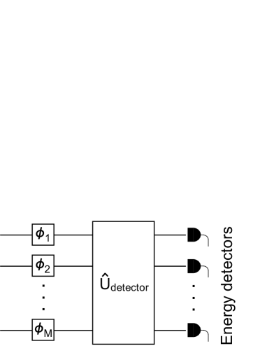
FIG. 3.: A schematic diagram of an interferometric measurement that also gives the total energy of the measured state. The interference of the $M$ modes is characterized by the lossless and unitary transformation $\hat{U}_{\rm detector}$.

In an earlier paper [16], we claimed that if $|\xi\rangle$ is a two-mode state, $\hat{U}_{\rm PS}(\phi)=\exp(i\phi[\hat{n}_{1}-\hat{n}_{2}]/2)$ is the two-mode unitary relative-phase shifting operator, and if

$$\langle\xi|\hat{U}_{\rm PS}(\phi)|\xi\rangle=0$$ (30)

can be fulfilled for some value of $\phi$, then “Eq. (30) constitutes the mathematical criterion for a state with a well-defined relative phase.” It is clear that Eq. (30) is a special case of Eq. (1), and therefore constitutes the necessary and sufficient condition for a relative phase shift to be distinguishable. However, as the following example shows, this property should not be referred to as “well-defined relative phase.” Suppose that

$$|\xi\rangle=\frac{1}{\sqrt{2}}(|0,0\rangle+|0,1\rangle)=|0\rangle\otimes\frac{1}{\sqrt{2}}(|0\rangle+|1\rangle).$$ (31)

It is trivial to show that in this case Eq. (30) is fulfilled for $\phi=2\pi$. However, a product state where one of the constituent factors is a single mode vacuum state is hardly a sensible candidate for a state with a well-defined relative phase. This is confirmed by the relative-phase distribution functions, which are flat [17]. The conclusion is that the criterion for an operationally well-defined relative phase must be reformulated.

The constant relative-phase distribution functions of the state (31) are a consequence of the fact that the relative-phase and the total energy are compatible observables [18]. Since $\hat{U}_{\rm PS}(\phi)$ also commutes with the total photon number operator $\sum_{N=0}^{\infty}N\hat{\openone}_{N}$, any measurement of two-mode relative phase (or visibility) will reveal the total photon number. Therefore, in order for the phase shift $\phi$ to be perfectly distinguishable, the phase-shifted state $\hat{U}_{\rm PS}(\phi)|\xi\rangle$ must, as in Eq. (28), become orthogonal to the original state $|\xi\rangle$ in every photon-number manifold. Consequently, the definition of well-defined relative phase should be refined as follows. If, for some phase shift $\phi$ and for all $N$, it is possible to fulfill

$$\langle\xi|\hat{\openone}_{N}\hat{U}_{\rm PS}(\phi)|\xi\rangle=0,$$ (32)

then the state $|\xi\rangle$ is said to have a well-defined relative phase. That any state fulfilling Eq. (32) also fulfills Eq. (30) can easily be verified. However, the converse is not true, as shown by the state (31), which does not fulfill Eq. (32).

Since all the components in different excitation manifolds must be made orthogonal simultaneously, the limits found in Sec. III imply that in this case $\phi\geq\pi/2N_{\rm max}$ and $\phi_{\rm tot}\geq\pi/N_{\rm max}$, where $N_{\rm max}$ denotes the highest excited manifold.

VI Discussion

We have found tight bounds set by the average energy of the used states on our accuracy measures $\phi$ and $\phi_{\rm tot}$. The bounds were derived for optical interferometers and pure states, but are obviously valid for other interfering bosons and mixed states, too. Our results also give tight bounds in the case where all phase shifts have the same sign. This would correspond to an experimental situation where there is a limited amount of phase-shift inducing material that can be distributed among the modes. Since the state (8) can saturate the bounds for $\phi_{\rm tot}$ with nonnegative or nonpositive phase shifts $\phi_{m}$ alone, the magnitude of the sum of these phase shifts has the same bounds for $N$-photon states and general states as $\phi_{\rm tot}$.

We would also like to point out that our results were derived from fundamental considerations. Apart from the brief discussion in Sec. V, we did not consider the problem of how to realize the measurements necessary to distinguish the optimal states. Although we have found that there is no fundamental advantage in using multimode interferometers in terms of their accuracy, they may offer simpler realizations compared to two-mode interferometers. For example, it may be easier to generate multimode states that give the same resolution as the two-mode states presented here.

Let us also comment on the earlier investigation of multimode interferometers by D’Ariano and Paris [13], which arrived at the conclusion that the multimode interferometers actually improve the accuracy. They considered interferometers whose phase shifts in the different modes were $\phi_{m}=m\varphi$. The “variance” of the estimate of $\varphi$ was found to be inversely proportional to the number of modes $M$, indicating that the accuracy in the measurement of $\varphi$ was improved correspondingly. However, we note that the largest relative phase shift $\phi_{M}-\phi_{1}=(M-1)\varphi$ increases with the number of modes $M$. Since the two-mode interferometer employs a relative phase shift of $\varphi$ instead of $(M-1)\varphi$, its sensitivity is not maximized. The relative phase shift $(M-1)\varphi$ would obviously give the same improvement in the accuracy of $\varphi$ for a two-mode interferometer as D’Ariano and Paris found for the $M$-mode interferometer. Therefore, we conclude that for a given average energy the ultimate phase-shift resolution of an interferometer is independent of the number of interfering modes.

REFERENCES

- [1] C. M. Caves, Phys. Rev. Lett. 45, 75 (1980).
- [2] Z. Y. Ou, Phys. Rev. Lett. 77, 2352 (1996).
- [3] C. M. Caves, Phys. Rev. D 23, 1693 (1981).
- [4] M. J. Holland and K. Burnett, Phys. Rev. Lett. 71, 1355 (1993).
- [5] J. Jacobson, G. Björk, I. Chuang, and Y. Yamamoto, Phys. Rev. Lett. 74, 4835 (1995).
- [6] J. J. Bollinger, W. M. Itano, D. J. Wineland, and D. J. Heinzen, Phys. Rev. A 54, R4649 (1996).
- [7] M. Xiao, L.-A. Wu, and H. J. Kimble, Phys. Rev. Lett. 59, 278 (1987).
- [8] P. Grangier, R. E. Slusher, B. Yurke, and A. LaPorta, Phys. Rev. Lett. 59, 2153 (1987).
- [9] A. Heidmann, R. J. Horowicz, S. Reynaud, E. Giacobino, C. Fabre, and G. Camy, Phys. Rev. Lett. 59, 2555 (1987).
- [10] J. L. Sørensen, J. Hald, and E. S. Polzik, Phys. Rev. Lett. 80, 3487 (1998).
- [11] N. Margolus and L. B. Levitin, Physica D 120, 188 (1998).
- [12] J. Söderholm, G. Björk, T. Tsegaye, and A. Trifonov, Phys. Rev. A 59, 1788 (1999).
- [13] G. M. D’Ariano and M. G. A. Paris, Phys. Rev. A 55, 2267 (1997).
- [14] B. C. Sanders, H. de Guise, D. J. Rowe, and A. Mann, J. Phys. A 32, 7791 (1999).
- [15] D. G. Blair, The detection of gravitational waves (Cambridge University Press, Cambridge, 1991).
- [16] G. Björk, S. Inoue, and J. Söderholm, Phys. Rev. A 62, 023817 (2000).
- [17] G. Björk, J. Söderholm, A. Trifonov, and T. Tsegaye, Phys. Scr. (to be published).
- [18] A. Luis and L. L. Sánchez-Soto, Phys. Rev. A 48, 4702 (1993).