Quantum search by measurement

Abstract

We propose a quantum algorithm for solving combinatorial search problems that uses only a sequence of measurements. The algorithm is similar in spirit to quantum computation by adiabatic evolution, in that the goal is to remain in the ground state of a time-varying Hamiltonian. Indeed, we show that the running times of the two algorithms are closely related. We also show how to achieve the quadratic speedup for Grover’s unstructured search problem with only two measurements. Finally, we discuss some similarities and differences between the adiabatic and measurement algorithms.

I Introduction

In the conventional circuit model of quantum computation, a program for a quantum computer consists of a discrete sequence of unitary gates chosen from a fixed set. The memory of the quantum computer is a collection of qubits initially prepared in some definite state. After a sequence of unitary gates is applied, the qubits are measured in the computational basis to give the result of the computation, a classical bit string.

This description of a quantum computer has been used to formulate quantum algorithms that outperform classical methods, notably Shor’s factoring algorithm Sho94 and Grover’s algorithm for unstructured search Gro97 . Subsequent development of quantum algorithms has focused primarily on variations of the techniques introduced by Shor and Grover. One way to motivate new algorithmic ideas is to consider alternative (but in general, equivalent) descriptions of the way a quantum computer operates. For example, the technique of quantum computation by adiabatic evolution FGGS00 is most easily described by a quantum computer that evolves continuously according to a time-varying Hamiltonian.

Another model of quantum computation allows measurement at intermediate stages. Indeed, recent work has shown that measurement alone is universal for quantum computation: one can efficiently implement a universal set of quantum gates using only measurements (and classical processing) Nie01 ; FZ01 ; Leu01 ; RB00 . In this paper, we describe an algorithm for solving combinatorial search problems that consists only of a sequence of measurements. Using a straightforward variant of the quantum Zeno effect (see for example Neu32 ; AV80 ; SRM93 ), we show how to keep the quantum computer in the ground state of a smoothly varying Hamiltonian $H(s)$. This process can be used to solve a computational problem by encoding the solution to the problem in the ground state of the final Hamiltonian.

The organization of the paper is as follows. In Section II, we present the algorithm in detail and describe how measurement of $H(s)$ can be performed on a digital quantum computer. In Section III, we estimate the running time of the algorithm in terms of spectral properties of $H(s)$. Then, in Section IV, we discuss how the algorithm performs on Grover’s unstructured search problem and show that by a suitable modification, Grover’s quadratic speedup can be achieved by the measurement algorithm. Finally, in Section V, we discuss the relationship between the measurement algorithm and quantum computation by adiabatic evolution.

II The measurement algorithm

Our algorithm is conceptually similar to quantum computation by adiabatic evolution FGGS00 , a general method for solving combinatorial search problems using a quantum computer. Both algorithms operate by remaining in the ground state of a smoothly varying Hamiltonian $H(s)$ whose initial ground state is easy to construct and whose final ground state encodes the solution to the problem. However, whereas adiabatic quantum computation uses Schrödinger evolution under $H(s)$ to remain in the ground state, the present algorithm uses only measurement of $H(s)$.

In general, we are interested in searching for the minimum of a function $h(z)$ that maps $n$-bit strings to positive real numbers. Many computational problems can be cast as minimization of such a function; for specific examples and their relationship to adiabatic quantum computation, see FGGS00 ; CFGG01 . Typically, we can restrict our attention to the case where the global minimum of $h(z)$ is unique. Associated with this function, we can define a problem Hamiltonian $H_{P}$ through its action on computational basis states:

$$H_{P}|z\rangle=h(z)|z\rangle\,.$$ (1)

Finding the global minimum of $h(z)$ is equivalent to finding the ground state of $H_{P}$. If the global minimum is unique, then this ground state is nondegenerate.

To reach the ground state of $H_{P}$, we begin with the quantum computer prepared in the ground state of some other Hamiltonian $H_{B}$, the beginning Hamiltonian. Then we consider a one-parameter family of Hamiltonians $H(s)$ that interpolates smoothly from $H_{B}$ to $H_{P}$ for $s\in[0,1]$. In other words, $H(0)=H_{B}$ and $H(1)=H_{P}$, and the intermediate $H(s)$ is a smooth function of $s$. One possible choice is linear interpolation,

$$H(s)=(1-s)H_{B}+sH_{P}\,.$$ (2)

Now we divide the interval $[0,1]$ into $M$ subintervals of width $\delta=1/M$. So long as the interpolating Hamiltonian $H(s)$ is smoothly varying and $\delta$ is small, the ground state of $H(s)$ will be close to the ground state of $H(s+\delta)$. Thus, if the system is in the ground state of $H(s)$ and we measure $H(s+\delta)$, the post-measurement state is very likely to be the ground state of $H(s+\delta)$. If we begin in the ground state of $H(0)$ and successively measure $H(\delta),H(2\delta),\ldots,H((M-1)\delta),H(1)$, then the final state will be the ground state of $H(1)$ with high probability, assuming $\delta$ is sufficiently small.

To complete our description of the quantum algorithm, we must explain how to measure the operator $H(s)$. The technique we use is motivated by von Neumann’s description of the measurement process Neu32 . In this description, measurement is performed by coupling the system of interest to an ancillary system, which we call the pointer. Suppose that the pointer is a one-dimensional free particle and that the system-pointer interaction Hamiltonian is $H(s)\otimes p$, where $p$ is the momentum of the particle. Furthermore, suppose that the mass of the particle is sufficiently large that we can neglect the kinetic term. Then the resulting evolution is

$$e^{-itH(s)\otimes p}=\sum_{a}\left[|E_{a}(s)\rangle\langle E_{a}(s)|\otimes e^{-itE_{a}(s)p}\right]\,,$$ (3)

where $|E_{a}(s)\rangle$ are the eigenstates of $H(s)$ with eigenvalues $E_{a}(s)$, and we have set $\hbar=1$. Suppose we prepare the pointer in the state $|x=0\rangle$, a narrow wave packet centered at $x=0$. Since the momentum operator generates translations in position, the above evolution performs the transformation

$$|E_{a}(s)\rangle\otimes|x=0\rangle\to|E_{a}(s)\rangle\otimes|x=tE_{a}(s)\rangle\,.$$ (4)

If we can measure the position of the pointer with sufficiently high precision that all relevant spacings $x_{ab}=t|E_{a}(s)-E_{b}(s)|$ can be resolved, then measurement of the position of the pointer — a fixed, easy-to-measure observable, independent of $H(s)$ — effects a measurement of $H(s)$.

Von Neumann’s measurement protocol makes use of a continuous variable, the position of the pointer. To turn it into an algorithm that can be implemented on a fully digital quantum computer, we can approximate the evolution (3) using $r$ quantum bits to represent the pointer Wie96 ; Zal98 . The full Hilbert space is thus a tensor product of a $2^{n}$-dimensional space for the system and a $2^{r}$-dimensional space for the pointer. We let the computational basis of the pointer, with basis states $\{|z\rangle\}$, represent the basis of momentum eigenstates. The label $z$ is an integer between $0$ and $2^{r}-1$, and the $r$ bits of the binary representation of $z$ specify the states of the $r$ qubits. In this basis, the digital representation of $p$ is

$$p=\sum_{j=1}^{r}2^{-j}{1-\sigma_{z}^{(j)}\over 2}\,,$$ (5)

a sum of diagonal operators, each of which acts on only a single qubit. Here $\sigma_{z}^{(j)}$ is the Pauli $z$ operator on the $j$th qubit. As we will discuss in the next section, we have chosen to normalize $p$ so that

$$p|z\rangle={z\over 2^{r}}|z\rangle\,,$$ (6)

which gives $\left\|p\right\|\sim 1$. If $H(s)$ is a sum of terms, each of which acts on at most $k$ qubits, then $H(s)\otimes p$ is a sum of terms, each of which acts on at most $k+1$ qubits. As long as $k$ is a fixed constant independent of the problem size $n$, such a Hamiltonian can be simulated efficiently on a quantum computer Llo96 . Expanded in the momentum eigenbasis, the initial state of the pointer is

$$|x=0\rangle={1\over 2^{r/2}}\sum_{z=0}^{2^{r}-1}|z\rangle\,.$$ (7)

The measurement is performed by evolving under $H(s)\otimes p$ for a total time $\tau$. We discuss how to choose $\tau$ in the next section. After this evolution, the position of the simulated pointer could be measured by measuring the qubits that represent it in the $x$ basis, i.e., the Fourier transform of the computational basis. However, note that our algorithm only makes use of the post-measurement state of the system, not of the measured value of $H(s)$. In other words, only the reduced density matrix of the system is relevant. Thus it is not actually necessary to perform a Fourier transform before measuring the pointer, or even to measure the pointer at all. When the system-pointer evolution is finished, one can either re-prepare the pointer in its initial state $|x=0\rangle$ or discard it and use a new pointer, and immediately begin the next measurement.

As an aside, note that the von Neumann measurement procedure described above is identical to the well-known phase estimation algorithm for measuring the eigenvalues of a unitary operator Kit95 ; CEMM98 , which can also be used to produce eigenvalues and eigenvectors of a Hamiltonian AL99 . This connection has been noted previously in Zal98 , and it has been pointed out that the measurement is a non-demolition measurement in TMR02 . In the phase estimation problem, we are given an eigenvector $|\psi\rangle$ of a unitary operator $U$ and asked to determine its eigenvalue $e^{-i\phi}$. The algorithm uses two registers, one that initially stores $|\psi\rangle$ and one that will store an approximation of the phase $\phi$. The first and last steps of the algorithm are Fourier transforms on the phase register. The intervening step is to perform the transformation

$$|\psi\rangle\otimes|z\rangle\to U^{z}|\psi\rangle\otimes|z\rangle\,,$$ (8)

where $|z\rangle$ is a computational basis state. If we take $|z\rangle$ to be a momentum eigenstate with eigenvalue $z$ (i.e., if we choose a different normalization than in (6)) and let $U=e^{-iHt}$, this is exactly the transformation induced by $e^{-i(H\otimes p)t}$. Thus we see that the phase estimation algorithm for a unitary operator $U$ is exactly von Neumann’s prescription for measuring $i\ln U$.

III Running time

The running time of the measurement algorithm is the product of $M$, the number of measurements, and $\tau$, the time per measurement. Even if we assume perfect projective measurements, the algorithm is guaranteed to keep the computer in the ground state of $H(s)$ only in the limit $M\to\infty$, so that $\delta=1/M\to 0$. Given a finite running time, the probability of finding the ground state of $H_{P}$ with the last measurement will be less than 1. To understand the efficiency of the algorithm, we need to determine how long we must run as a function of $n$, the number of bits on which the function $h$ is defined, so that the probability of success is not too small. In general, if the time required to achieve a success probability greater than some fixed constant (e.g., $1\over 2$) is $\mathop{\mathrm{poly}}(n)$, we say the algorithm is efficient, whereas if the running time grows exponentially, we say it is not.

To determine the running time of the algorithm, we consider the effect of the measurement process on the reduced density matrix of the system. Here, we simply motivate the main result; for a detailed analysis, see Appendix A.

Let $\rho^{(j)}$ denote the reduced density matrix of the system after the $j$th measurement; its matrix elements are

$$\rho^{(j)}_{ab}=\langle E_{a}(j\delta)|\rho^{(j)}|E_{b}(j\delta)\rangle\,.$$ (9)

The interaction with the digitized pointer effects the transformation

$$|E_{a}(s)\rangle\otimes|z\rangle\to e^{-iE_{a}(s)zt/2^{r}}|E_{a}(s)\rangle\otimes|z\rangle\,.$$ (10)

Starting with the pointer in the state (7), evolving according to (10), and tracing over the pointer, the quantum operation induced on the system is

$$\rho^{(j+1)}_{ab}=\kappa^{(j+1)}_{ab}\sum_{c,d}U^{(j)}_{ac}\rho^{(j)}_{cd}U^{(j)*}_{bd}\,,$$ (11)

where the unitary transformation relating the energy eigenbases at $s=j\delta$ and $s=(j+1)\delta$ is

$$U^{(j)}_{ab}=\langle E_{a}((j+1)\delta)|E_{b}(j\delta)\rangle$$ (12)

and

$$\kappa^{(j)}_{ab}={1\over 2^{r}}\sum_{z=0}^{2^{r}-1}e^{i[E_{b}(j\delta)-E_{a}(j\delta)]zt/2^{r}}\,.$$ (13)

Summing this geometric series, we find

$$\left|\kappa^{(j)}_{ab}\right|^{2}=\left|\kappa([E_{b}(j\delta)-E_{a}(j\delta)]t/2)\right|^{2}\,,$$ (14)

where

$$|\kappa(x)|^{2}={\sin^{2}x\over 4^{r}\sin^{2}(x/2^{r})}\,.$$ (15)

This function is shown in Fig. 1 for the case $r=4$. It has a sharp peak of unit height and width of order 1 at the origin, and identical peaks at integer multiples of $2^{r}\pi$.

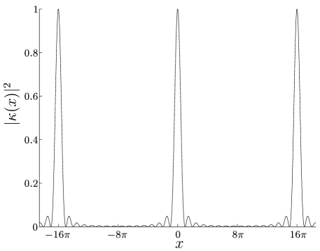
Figure 1: The function $|\kappa(x)|^{2}$ for $r=4$.

If the above procedure were a perfect projective measurement, then we would have $\kappa_{ab}=0$ whenever $E_{a}\neq E_{b}$. Assuming (temporarily) that this is the case, we find

$$\rho^{(j+1)}_{00}\geq\left|U^{(j)}_{00}\right|^{2}\rho^{(j)}_{00}$$ (16)

with the initial condition $\rho^{(0)}_{00}=1$ and $\rho^{(0)}_{ab}=0$ otherwise. Perturbation theory gives

$$\left|U^{(j)}_{00}\right|^{2} = 1-\delta^{2}\sum_{a\neq 0}{|\langle E_{a}(s)|{{\mathrm{d}}H\over{\mathrm{d}}s}|E_{0}(s)\rangle|^{2}\over(E_{0}(s)-E_{a}(s))^{2}}\Bigg{|}_{s=j\delta}$$ (17)

$$+O(\delta^{3})$$

$$\geq 1-{\Gamma(j\delta)^{2}\,\delta^{2}\over g(j\delta)^{2}}+O(\delta^{3})\,,$$ (18)

where

$$\Gamma(s)^{2}=\langle E_{0}(s)|({\textstyle{{\mathrm{d}}H\over{\mathrm{d}}s}})^{2}|E_{0}(s)\rangle-\langle E_{0}(s)|{\textstyle{{\mathrm{d}}H\over{\mathrm{d}}s}}|E_{0}(s)\rangle^{2}$$ (19)

and

$$g(s)=E_{1}(s)-E_{0}(s)$$ (20)

is the energy gap between the ground and first excited states. If we let

$$\Gamma = \max_{s\in[0,1]}\Gamma(s)$$ (21)

$$g = \min_{s\in[0,1]}g(s)\,,$$ (22)

then according to (16), the probability of being in the ground state after the last measurement is at least

$$\rho^{(M)}_{00} \geq \left[1-{\Gamma^{2}\over M^{2}g^{2}}+O(M^{-3})\right]^{M}$$ (23)

$$= \exp\left(-{\Gamma^{2}\over Mg^{2}}\right)+O(M^{-2})\,.$$ (24)

The probability of success is close to 1 provided

$$M\gg{\Gamma^{2}\over g^{2}}\,.$$ (25)

When $H_{B}$ and $H_{P}$ are both sums of $\mathop{\mathrm{poly}}(n)$ terms, each of which acts nontrivially on at most a constant number of qubits, it is easy to choose an interpolation such as (2) so that $\Gamma$ is only $\mathop{\mathrm{poly}}(n)$. Thus we are mainly interested in the behavior of $g$, the minimum gap between the ground and first excited states. We see that for the algorithm to be successful, the total number of measurements must be much larger than $1/g^{2}$.

In fact, the simulated von Neumann procedure is not a perfect projective measurement. We must determine how long the system and pointer should interact so that the measurement is sufficiently good. The analysis in Appendix A shows that $|\kappa^{(j)}_{01}|^{2}$ should be bounded below 1 by a constant for all $j$. In other words, to sufficiently resolve the difference between the ground and first excited states, we must decrease the coherence between them by a fixed fraction per measurement. The width of the central peak in Fig. 1 is of order 1, so it is straightforward to show that to have $|\kappa(x)|^{2}$ less than, say, $1/2$, we must have $x\geq O(1)$. This places a lower bound on the system-pointer interaction time of

$$\tau\geq{O(1)\over g}$$ (26)

independent of $r$, the number of pointer qubits. (Note that the same bound also holds in the case of a continuous pointer with a fixed resolution length.)

Putting these results together, we find that the measurement algorithm is successful if the total running time, $T=M\tau$, satisfies

$$T\gg{\Gamma^{2}\over g^{3}}\quad\textrm{(measurement)}\,.$$ (27)

This result can be compared to the corresponding expression for quantum computation by adiabatic evolution,

$$T\gg{\Gamma\over g^{2}}\quad\textrm{(adiabatic)}\,.$$ (28)

Note that the same quantity appears in the numerator of both expressions; in both cases, $\Gamma$ accounts for the possibility of transitions to all possible excited states.

The adiabatic and measurement algorithms have qualitatively similar behavior: if the gap is exponentially small, neither algorithm is efficient, whereas if the gap is only polynomially small, both algorithms are efficient. However, the measurement algorithm is slightly slower: whereas adiabatic evolution runs in a time that grows like $1/g^{2}$, the measurement algorithm runs in a time that grows like $1/g^{3}$. To see that this comparison is fair, recall that we have defined the momentum in (5) so that $||p||\sim 1$, which gives $||H(s)||\sim||H(s)\otimes p||$. Alternatively, we can compare the number $\eta$ of few-qubit unitary gates needed to simulate the two algorithms on a conventional quantum computer. Using the Lie product formula

$$e^{A+B}\simeq(e^{A/m}e^{B/m})^{m}\,,$$ (29)

which is valid provided $m\gg\left\|A\right\|^{2}+\left\|B\right\|^{2}$, we find $\eta=O(1/g^{4})$ for adiabatic evolution and $\eta=O(1/g^{6})$ for the measurement algorithm, in agreement with the previous comparison.

The argument we have used to motivate (27) is explained in greater detail in Appendix A. There, we also consider the number of qubits, $r$, that must be used to represent the pointer. We show that if the gap is only polynomially small in $n$, it is always sufficient to take $r=O(\log n)$. However, we argue that generally a single qubit will suffice.

IV The Grover problem

The unstructured search problem considered by Grover is to find a particular unknown $n$-bit string $w$ (the marked state, or the winner) using only queries of the form “is $z$ the same as $w$?” Gro97 . In other words, one is trying to minimize a function

$$h_{w}(z)=\left\{\matrix{0\,,\quad z=w\cr 1\,,\quad z\neq w}\right.\,.$$ (30)

Since there are $2^{n}$ possible values for $w$, the best possible classical algorithm uses $\Theta(2^{n})$ queries. However, Grover’s algorithm requires only $\Theta(2^{n/2})$ queries, providing a (provably optimal BBBV97 ) quadratic speedup. In Grover’s algorithm, the winner is specified by an oracle $U_{w}$ with

$$U_{w}|z\rangle=(-1)^{h_{w}(z)}|z\rangle\,.$$ (31)

This oracle is treated as a black box that one can use during the computation. One call to this black box is considered to be a single query of the oracle.

In addition to Grover’s original algorithm, quadratic speedup can also be achieved in a time-independent Hamiltonian formulation FG98a or by adiabatic quantum computation RC01 ; DMV01 . In either of these formulations, the winner is specified by an “oracle Hamiltonian”

$$H_{w}=1-|w\rangle\langle w|$$ (32)

whose ground state is $|w\rangle$ and that treats all orthogonal states (the non-winners) equivalently. One is provided with a black box that implements $H_{w}$, where $w$ is unknown, and is asked to find $w$. Instead of counting queries, the efficiency of the algorithm is quantified in terms of the total time for which one applies the oracle Hamiltonian.

Here, we show that if we are given a slightly different black box, we can achieve quadratic speedup using the measurement algorithm. We let the problem Hamiltonian be $H_{P}=H_{w}$ and we consider a one-parameter family of Hamiltonians $H(s)$ given by (2) for some $H_{B}$. Because we would like to measure this Hamiltonian, it is not sufficient to be given a black box that allows one to evolve the system according to $H_{w}$. Instead, we will use a black box that evolves the system and a pointer according to $H_{w}\otimes p$, where $p$ is the momentum of the pointer. This oracle is compared to the previous two in Fig. 2. By repeatedly alternating between applying this black box and evolving according to $H_{B}\otimes p$, each for small time, we can produce an overall evolution according to the Hamiltonian $[sH_{B}+(1-s)H_{P}]\otimes p$, and thus measure the operator $H(s)$ for any $s$.

Figure 2: Oracles for the Grover problem. (a) Top: Grover’s original oracle. (b) Center: An oracle that performs evolution according to $H_{w}$. The double line indicates a classical control parameter, the time for which the Hamiltonian is applied. (c) Bottom: An oracle that allows one to measure $H_{w}$.

Now consider the beginning Hamiltonian

$$H_{B}=\sum_{j}{1-\sigma_{x}^{(j)}\over 2}\,,$$ (33)

where $\sigma_{x}^{(j)}$ is the Pauli $x$ operator acting on the $j$th qubit. This beginning Hamiltonian is a sum of local terms, and has the easy-to-prepare ground state $|E_{0}(0)\rangle=2^{-n/2}\sum_{z}|z\rangle$, the uniform superposition of all possible bit strings in the computational basis. If we consider the interpolation (2), then one can show FGGS00 that the minimum gap occurs at

$$s^{*}=1-{2\over n}+O(n^{-2})\,,$$ (34)

where the gap takes the value

$$g(s^{*})=2^{1-n/2}[1+O(n^{-1})]\,.$$ (35)

Naively applying (27) gives a running time $T=O(2^{3n/2})$, which is even worse than the classical algorithm.

However, since we know the value of $s^{*}$ independent of $w$, we can improve on this approach by making fewer measurements. We observe that in the limit of large $n$, the ground state of $H(s)$ is close to the ground state $|E_{0}(0)\rangle$ of $H_{B}$ for $s\lesssim s^{*}$ and is close to the ground state $|E_{0}(1)\rangle=|w\rangle$ of $H_{P}$ for $s\gtrsim s^{*}$, switching rapidly from one state to the other in the vicinity of $s=s^{*}$. In Appendix B, we show that up to terms of order $1/n$, the ground state $|\psi_{+}\rangle$ and the first excited state $|\psi_{-}\rangle$ of $H(s^{*})$ are the equal superpositions

$$|\psi_{\pm}\rangle\simeq{1\over\sqrt{2}}(|E_{0}(0)\rangle\pm|E_{0}(1)\rangle)$$ (36)

of the initial and final ground states (which are nearly orthogonal for large $n$). If we prepare the system in the state $|E_{0}(0)\rangle$ and make a perfect measurement of $H(s^{*})$ followed by a perfect measurement of $H(1)$, we find the result $w$ with probability $1\over 2$. The same effect can be achieved with an imperfect measurement, even if the pointer consists of just a single qubit. First consider the measurement of $H(s^{*})$ in the state $|E_{0}(0)\rangle$. After the system and pointer have interacted for a time $t$ according to (10) with $r=1$, the reduced density matrix of the system in the $\{|\psi_{+}\rangle,|\psi_{-}\rangle\}$ basis is approximately

$${1\over 2}\left(\matrix{1&e^{ig(s^{*})t/4}\cos[g(s^{*})t/4]\cr e^{-ig(s^{*})t/4}\cos[g(s^{*})t/4]&1}\right)\,.$$ (37)

If we then measure $H(1)$ (i.e., measure in the computational basis), the probability of finding $w$ is approximately

$${1\over 2}\sin^{2}[g(s^{*})t/4]\,.$$ (38)

To get an appreciable probability of finding $w$, we choose $t=\Theta(2^{n/2})$.

This approach is similar to the way one can achieve quadratic speedup with the adiabatic algorithm. Schrödinger time evolution governed by (2) does not yield quadratic speedup. However, because $s^{*}$ is independent of $w$, we can change the Hamiltonian quickly when the gap is big and more slowly when the gap is small. Since the gap is only of size $\sim 2^{-n/2}$ for a region of width $\sim 2^{-n/2}$, the total oracle time with this modified schedule need only be $O(2^{n/2})$. This has been demonstrated explicitly by solving for the optimal schedule using a different beginning Hamiltonian $H_{B}^{\prime}$ that is not a sum of local terms RC01 ; DMV01 , but it also holds using the beginning Hamiltonian (33).

Note that measuring $H(s^{*})$ is not the only way to solve the Grover problem by measurement. More generally, we can start in some $w$-independent state, measure the operator

$$\tilde{H}=H_{w}+K$$ (39)

where $K$ is also independent of $w$, and then measure in the computational basis. For example, suppose we choose

$$K=1-|\psi\rangle\langle\psi|\,,$$ (40)

where $|\psi\rangle$ is a $w$-independent state with the property $|\langle w|\psi\rangle|\sim 2^{-n/2}$ for all $w$. (If we are only interested in the time for which we use the black box shown in Fig. 2(c), i.e., if we are only interested in the oracle query complexity, then we need not restrict $K$ to be a sum of local terms.) In (40), the coefficient of $-1$ in front of $|\psi\rangle\langle\psi|$ has been fine-tuned so that $|\psi\rangle+|w\rangle$ is the ground state of $\tilde{H}$ (choosing the phase of $|w\rangle$ so that $\langle w|\psi\rangle$ is real and positive). If the initial state has a large overlap with $|\psi\rangle$, then the measurement procedure solves the Grover problem. However, the excited state $|\psi\rangle-|w\rangle$ is also an eigenstate of $\tilde{H}$, with an energy higher by of order $2^{-n/2}$. Thus the time to perform the measurement must be $\Omega(2^{n/2})$.

The measurement procedures described above saturate the well-known lower bound on the time required to solve the Grover problem. Using an oracle like the one shown in Fig. 2(a), Bennett et al. showed that the Grover problem cannot be solved on a quantum computer using fewer than of order $2^{n/2}$ oracle queries BBBV97 . By a straightforward modification of their argument, an equivalent result applies using the oracle shown in Fig. 2(c). Thus every possible $\tilde{H}$ as in (39) that can be measured to find $w$ must have a gap between the energies of the relevant eigenstates of order $2^{-n/2}$ or smaller.

V Discussion

We have described a way to solve combinatorial search problems on a quantum computer using only a sequence of measurements to keep the computer near the ground state of a smoothly varying Hamiltonian. The basic principle of this algorithm is similar to quantum computation by adiabatic evolution, and the running times of the two methods are closely related. Because of this close connection, many results on adiabatic quantum computation can be directly imported to the measurement algorithm — for example, its similarities and differences with classical simulated annealing FGG02 . We have also shown that the measurement algorithm can achieve quadratic speedup for the Grover problem using knowledge of the place where the gap is smallest, as in adiabatic quantum computation.

One of the advantages of adiabatic quantum computation is its inherent robustness against error CFP02 . In adiabatic computation, the particular path from $H_{B}$ to $H_{P}$ is unimportant as long as the initial and final Hamiltonians are correct, the path is smoothly varying, and the minimum gap along the path is not too small. Exactly the same considerations apply to the measurement algorithm. However, the adiabatic algorithm also enjoys robustness against thermal transitions out of the ground state: if the temperature of the environment is much smaller than the gap, then such transitions are suppressed. The measurement algorithm might not possess this kind of robustness, since the Hamiltonian of the quantum computer during the measurement procedure is not simply $H(s)$.

Although it does not provide a computational advantage over quantum computation by adiabatic evolution, the measurement algorithm is an alternative way to solve general combinatorial search problems on a quantum computer. The algorithm can be simply understood in terms of measurements of a set of operators, without reference to unitary time evolution. Nevertheless, we have seen that to understand the running time of the algorithm, it is important to understand the dynamical process by which these measurements are realized.

Appendix A The measurement process

In Section III, we discussed the running time of the measurement algorithm by examining the measurement process. In this Appendix, we present the analysis in greater detail. First, we derive the bound on the running time by demonstrating (25) and (26). We show rigorously that these bounds are sufficient as long as the gap is only polynomially small and the number of qubits used to represent the pointer is $r=O(\log n)$. Finally, we argue that $r=1$ qubit should be sufficient in general.

Our goal is to find a bound on the final success probability of the measurement algorithm. We consider the effect of the measurements on the reduced density matrix of the system, which can be written as the block matrix

$$\rho=\left(\matrix{\mu&\nu^{\dagger}\cr\nu&\chi}\right)$$ (41)

where $\mu=\rho_{00}$, $\nu_{a}=\rho_{a0}$ for $a\neq 0$, and $\chi_{ab}=\rho_{ab}$ for $a,b\neq 0$. Since $\mathop{\mathrm{tr}}\rho=1$, $\mu=1-\mathop{\mathrm{tr}}\chi$. For ease of notation, we suppress $j$, the index of the iteration, except where necessary. The unitary transformation (12) may also be written as a block matrix. Define $\epsilon=\Gamma\delta/g$. Using perturbation theory and the unitarity constraint, we can write

$$U=\left(\matrix{u&-w^{\dagger}V+O(\epsilon^{3})\cr w&V+O(\epsilon^{2})}\right)\,,$$ (42)

where $|u|^{2}\geq 1-\epsilon^{2}+O(\epsilon^{3})$, $\left\|w\right\|^{2}\leq\epsilon^{2}+O(\epsilon^{3})$, and $V$ is a unitary matrix. We let $\left\|\cdot\right\|$ denote the $l_{2}$ vector or matrix norm as appropriate. Furthermore, let

$$\kappa=\left(\matrix{1&k^{\dagger}\cr k&J}\right)\,.$$ (43)

From (11), the effect of a single measurement may be written

$$\rho^{\prime}=(U\rho U^{\dagger})\circ\kappa\,,$$ (44)

where $\circ$ denotes the element-wise (Hadamard) product. If we assume $\left\|\nu\right\|=O(\epsilon)$, we find

$$\mu^{\prime} = |u|^{2}\mu-w^{\dagger}V\nu-\nu^{\dagger}V^{\dagger}w+O(\epsilon^{3})$$ (45)

$$\nu^{\prime} = [V\nu+\mu w-V\chi V^{\dagger}w+O(\epsilon^{2})]\circ k\,.$$ (46)

Now we use induction to show that our assumption always remains valid. Initially, $\nu^{(0)}=0$. Using the triangle inequality in (46), we find

$$\left\|\nu^{\prime}\right\|\leq[\left\|\nu\right\|+\epsilon+O(\epsilon^{2})]\tilde{k}\,,$$ (47)

where

$$\tilde{k}=\max_{j,a}\left|k^{(j)}_{a}\right|\,.$$ (48)

So long as $\tilde{k}<1$, we can sum a geometric series, extending the limits to go from $0$ to $\infty$, to find

$$\left\|\nu^{(j)}\right\|\leq{\epsilon\over 1-\tilde{k}}+O(\epsilon^{2})$$ (49)

for all $j$. In other words, $\left\|\nu\right\|=O(\epsilon)$ so long as $\tilde{k}$ is bounded below 1 by a constant.

Finally, we put a bound on the final success probability $\mu^{(M)}$. Using the Cauchy-Schwartz inequality in (45) gives

$$\mu^{\prime}\geq(1-\epsilon^{2})\mu-{2\epsilon^{2}\over 1-\tilde{k}}+O(\epsilon^{3})\,.$$ (50)

Iterating this bound $M$ times with the initial condition $\mu^{(0)}=1$, we find

$$\mu^{(M)}\geq 1-{\Gamma^{2}\over Mg^{2}}\left(1+{2\over 1-\tilde{k}}\right)+O(M\epsilon^{3})\,.$$ (51)

If $\tilde{k}$ is bounded below 1 by a constant (independent of $n$), we find the condition (25) as claimed in Section III.

The requirement on $\tilde{k}$ gives the bound (26) on the measurement time $\tau$, and also gives a condition on the number of pointer qubits $r$. To see this, we must investigate properties of the function $|\kappa(x)|^{2}$ defined in (15) and shown in Fig. 1. It is straightforward to show that $|\kappa(x)|^{2}\leq 1/2$ for $\pi/2\leq x\leq\pi(2^{r}-1/2)$. Thus, if we want $\tilde{k}$ to be bounded below 1 by a constant, we require

$$\pi/2\leq[E_{a}(s)-E_{0}(s)]t/2\leq\pi(2^{r}-1/2)$$ (52)

for all $s$ and for all $a\neq 0$. The left hand bound with $a=1$ gives $t\geq\pi/g$, which is (26). Requiring the right hand bound to hold for the largest energy difference gives the additional condition $2^{r}\gtrsim(E_{2^{n}-1}-E_{0})/g$. Since we only consider Hamiltonians $H(s)$ that are sums of $\mathop{\mathrm{poly}}(n)$ terms of bounded size, the largest possible energy difference must be bounded by a polynomial in $n$. If we further suppose that $g$ is only polynomially small, this condition is satisfied by taking

$$r=O(\log n)\,,$$ (53)

as claimed at the end of Section III. Thus we see that the storage requirements for the pointer are rather modest.

However, the pointer need not comprise even this many qubits. Since the goal of the measurement algorithm is to keep the system close to its ground state, it would be surprising if the energies of highly excited states were relevant. Suppose we take $r=1$; then $|\kappa(x)|^{2}=\cos^{2}(x/2)$. As before, (26) suffices to make $|\kappa_{01}|^{2}$ sufficiently small. However, we must also consider terms involving $|\kappa_{0a}|^{2}$ for $a>1$. The algorithm will fail if the term $\mu w\circ k$ in (46) accumulates to be $O(1)$ over $M$ iterations. This will only happen if, for $O(M)$ iterations, most of $\left\|w\right\|$ comes from components $w_{a}$ with $(E_{a}-E_{0})t$ close to an integer multiple of $2\pi$. In such a special case, changing $t$ will avoid the problem. An alternative strategy would be to choose $t$ from a random distribution independently at each iteration.

Appendix B Eigenstates in the Grover problem

Here, we show that the ground state of $H(s^{*})$ for the Grover problem is close to (36). Our analysis follows Section 4.2 of FGGS00 .

Since the Grover problem is invariant under the choice of $w$, we consider the case $w=0$ without loss of generality. In this case, the problem can be analyzed in terms of the total spin operators

$$S_{a}={1\over 2}\sum_{j=1}^{n}\sigma_{a}^{(j)}\,,$$ (54)

where $a=x,y,z$ and $\sigma_{a}^{(j)}$ is the Pauli $a$ operator acting on the $j$th qubit. The Hamiltonian commutes with $\vec{S}^{2}=S_{x}^{2}+S_{y}^{2}+S_{z}^{2}$, and the initial state has $\vec{S}^{2}={n\over 2}({n\over 2}+1)$, so we can restrict our attention to the $(n+1)$-dimensional subspace of states with this value of $\vec{S}^{2}$. In this subspace, the eigenstates of the total spin operators satisfy

$$S_{a}|m_{a}=m\rangle=m|m_{a}=m\rangle$$ (55)

for $m=-{n\over 2},-{n\over 2}+1,\ldots,{n\over 2}$. Written in terms of the total spin operators and eigenstates, the Hamiltonian is

$$H(s) = (1-s)\left({n\over 2}-S_{x}\right)$$ (56)

$$+s\left(1-\left|m_{z}={n\over 2}\right\rangle\left\langle m_{z}={n\over 2}\right|\right)\,.$$

The initial and final ground states are given by $|E_{0}(0)\rangle=|m_{x}={n\over 2}\rangle$ and $|E_{0}(1)\rangle=|m_{z}={n\over 2}\rangle$, respectively.

Projecting the equation $H(s)|\psi\rangle=E|\psi\rangle$ onto the eigenbasis of $S_{x}$, we find

$$\left\langle m_{x}={n\over 2}-r\Big{|}\psi\right\rangle={s\over 1-s}{\sqrt{P_{r}}\over r-\lambda}\left\langle m_{z}={n\over 2}\Big{|}\psi\right\rangle\,,$$ (57)

where we have defined $\lambda=(E-s)/(1-s)$ and $P_{r}=2^{-n}{n\choose r}$. Now focus on the ground state $|\psi_{+}\rangle$ and the first excited state $|\psi_{-}\rangle$ of $H(s^{*})$. By equation (4.39) of FGGS00 , these states have $\lambda_{\pm}=\mp{n\over 2}2^{-n/2}(1+O(1/n))$. Putting $r=0$ in (57) and taking $s=s^{*}$ from (34), we find

$$\left\langle m_{x}={n\over 2}\Big{|}\psi_{\pm}\right\rangle=\pm\left\langle m_{z}={n\over 2}\Big{|}\psi_{\pm}\right\rangle(1+O(1/n))\,.$$ (58)

For $r\neq 0$, we have

$$\left\langle m_{x}={n\over 2}-r\Big{|}\psi_{\pm}\right\rangle = {n\over 2}{\sqrt{P_{r}}\over r}\left\langle m_{z}={n\over 2}\Big{|}\psi_{\pm}\right\rangle$$ (59)

$$\times(1+O(1/n))\,.$$

Requiring that $|\psi_{\pm}\rangle$ be normalized, we find

$$1 = \sum_{r=0}^{n}\left|\left\langle m_{x}={n\over 2}-r\Big{|}\psi_{\pm}\right\rangle\right|^{2}$$ (61)

$$= \left|\left\langle m_{z}={n\over 2}\Big{|}\psi_{\pm}\right\rangle\right|^{2}\left(1+{n^{2}\over 4}\sum_{r=1}^{n}{P_{r}\over r^{2}}\right)$$

$$\times(1+O(1/n))$$

$$= \left|\left\langle m_{z}={n\over 2}\Big{|}\psi_{\pm}\right\rangle\right|^{2}(2+O(1/n))\,,$$ (62)

which implies $|\langle m_{z}={n\over 2}|\psi_{\pm}\rangle|^{2}={1\over 2}+O(1/n)$. From (58), we also have $|\langle m_{x}={n\over 2}|\psi_{\pm}\rangle|^{2}={1\over 2}+O(1/n)$. Thus we find

$$|\psi_{\pm}\rangle\simeq{1\over\sqrt{2}}\left(\left|m_{x}={n\over 2}\right\rangle\pm\left|m_{z}={n\over 2}\right\rangle\right)$$ (63)

up to terms of order $1/n$, which is (36).

References

- (1) P. W. Shor, Algorithms for quantum computation: discrete logarithms and factoring, in Proc. 35th Annual Symposium on Foundations of Computer Science, ed. S. Goldwasser, 124 (IEEE Press, Los Alamitos, CA, 1994).
- (2) L. K. Grover, Quantum mechanics helps in searching for a needle in a haystack, Phys. Rev. Lett. 79, 325 (1997).
- (3) E. Farhi, J. Goldstone, S. Gutmann, and M. Sipser, Quantum computation by adiabatic evolution, quant-ph/0001106.
- (4) M. A. Nielsen, Universal quantum computation using only projective measurement, quantum memory, and preparation of the 0 state, quant-ph/0108020.
- (5) S. A. Fenner and Y. Zhang, Universal quantum computation with two- and three-qubit projective measurements, quant-ph/0111077.
- (6) D. W. Leung, Two-qubit projective measurements are universal for quantum computation, quant-ph/0111122.
- (7) R. Raussendorf and H. J. Briegel, Quantum computing via measurements only, quant-ph/0010033.
- (8) J. von Neumann, Mathematical Foundations of Quantum Mechanics (Princeton University Press, Princeton, NJ, 1955).
- (9) Y. Aharonov and M. Vardi, Meaning of an individual “Feynman path,” Phys. Rev. D 21, 2235 (1980).
- (10) L. S. Schulman, A. Ranfagni, and D. Mugnai, Characteristic scales for dominated time evolution, Physica Scripta 49, 536 (1993).
- (11) A. M. Childs, E. Farhi, J. Goldstone, and S. Gutmann, Finding cliques by quantum adiabatic evolution, quant-ph/0012104.
- (12) S. Wiesner, Simulations of many-body quantum systems by a quantum computer, quant-ph/9603028.
- (13) C. Zalka, Simulating quantum systems on a quantum computer, Proc. R. Soc. London A 454, 313 (1998).
- (14) S. Lloyd, Universal quantum simulators, Science 273, 1073 (1996).
- (15) A. Yu. Kitaev, Quantum measurements and the abelian stabilizer problem, quant-ph/9511026.
- (16) R. Cleve, A. Ekert, C. Macchiavello, and M. Mosca, Quantum algorithms revisited, Proc. R. Soc. London A 454, 339 (1998).
- (17) D. S. Abrams and S. Lloyd, Quantum algorithm providing exponential speed increase for finding eigenvalues and eigenvectors, Phys. Rev. Lett. 83, 5162 (1999).
- (18) B. C. Travaglione, G. J. Milburn, and T. C. Ralph, Phase estimation as a quantum nondemolition measurement, quant-ph/0203130.
- (19) C. H. Bennett, E. Bernstein, G. Brassard, and U. Vazirani, Strengths and weaknesses of quantum computing, SIAM J. Comput. 26, 1510 (1997).
- (20) E. Farhi and S. Gutmann, Analog analogue of a digital quantum computation, Phys. Rev. A 57, 2403 (1998).
- (21) J. Roland and N. Cerf, Quantum search by local adiabatic evolution, quant-ph/0107015.
- (22) W. van Dam, M. Mosca, and U. Vazirani, How powerful is adiabatic quantum computation?, to appear in FOCS 2001.
- (23) E. Farhi, J. Goldstone, and S. Gutmann, Quantum adiabatic evolution algorithms versus simulated annealing, quant-ph/0201031.
- (24) A. M. Childs, E. Farhi, and J. Preskill, Robustness of adiabatic quantum computation, Phys. Rev. A 65, 012322 (2002).