A scheme for direct observation of entanglement for Gaussian continuous variables

Abstract

We suggest an experimentally realizable scheme to test entanglement of a mixed Gaussian continuous variable state. We find that the entanglement condition is simplified for the family of Gaussian states which are relevant to experimental realization. The entanglement condition is then shown to be directly related to joint homodyne measurements. We show how robust the proposed test of entanglement is against imperfect detection efficiency.

In the current development of quantum information processing, entanglement, which is quantum correlation between particles, plays a critical role. Recently, the generation, manipulation and application of continuous-variable entangled states have been extensively studied Braunstein ; Ralph ; Plenio ; Leuchs mainly for Gaussian states. It is because the Gaussian continuous variables are extremely similar to qubit systems in theoretical treatment and they are the continuous-variable states that can be realized in a laboratory.

A state is said to be entangled when it is not separable. A Gaussian continuous-variable state is separable if and only if the partial transpose of its density matrix is non-negative Simon . This condition is equivalent to the possibility of imposing a positive well-defined $P$ function to the state after local unitary operations Duan ; LeeKim . In this paper, we show that the entanglement condition is simplified for a family of Gaussian states which are more relevant to experimental realization. We then suggest a scheme to test entanglement using joint homodyne measurements.

Einstein, Podolsky and Rosen (EPR) paradox is closely related to entanglement. There have been discussions on the EPR argument for continuous variables based on Bell’s inequality Banaszek ; Walmsley . On the other hand, Reid and Drummond Reid were concerned with the demonstration of the EPR paradox itself as distinct from Bell’s inequalities. They derived a noise level which is violated by the EPR paradox. Silberhorn et al. Leuchs proved the generation of an EPR entangled state by the indirect measure of the sub-vacuum noise in quadrature correlations. Even though the relation of EPR paradox to entanglement is still to be ravelled, it has been generally accepted that there is a subtle difference. We show that Reid and Drummond’s EPR criterion is only a sufficient condition for entanglement.

A two-mode Gaussian state is represented by a Gaussian Weyl characteristic function

$$C({\bf x})=\exp(-\frac{1}{2}{\bf x}{\bf V}{\bf x}^{T})$$ (1)

where ${\bf x}=(q_{1},p_{1},q_{2},p_{2})$, ${\bf x}^{T}$ is the transpose matrix of ${\bf x}$ and ${\bf V}$ is the quadrature matrix defined as $2\langle\{x_{i},x_{j}\}\rangle$. The quadrature variables $q_{i}$ and $p_{i}$ for mode $i(=1,2)$ correspond respectively to quadrature operators $\hat{q}_{i}=(\hat{a}_{i}+\hat{a}_{i}^{\dagger})/\sqrt{2}$ and $\hat{p}_{i}=i(\hat{a}_{i}-\hat{a}_{i}^{\dagger})/\sqrt{2}$ where $\hat{a}_{i}$ and $\hat{a}_{i}^{\dagger}$ are bosonic operators. The quadrature matrix can in fact be written using $2$ block matrices ${\bf L_{1}}$ and ${\bf L_{2}}$ for local quadrature variables and ${\bf C}$ and its transpose ${\bf C^{T}}$ representing inter-mode correlation,

$${\bf V}=\begin{pmatrix}{\bf L_{1}}&{\bf C}\\ {\bf C^{T}}&{\bf L_{2}}\\ \end{pmatrix}.$$ (2)

Lemma 1. — If the block matrices ${\bf L_{1}}={\bf L_{2}}$ and ${\bf C}$ are diagonal, i.e., the quadrature matrix of a Gaussian continuous-variable state has the following form:

$${\bf V}_{0}=\begin{pmatrix}n_{1}&0&c_{1}&0\\ 0&n_{2}&0&c_{2}\\ c_{1}&0&n_{1}&0\\ 0&c_{2}&0&n_{2}\end{pmatrix}$$ (3)

where $n_{1}$ or $n_{2}$ may be smaller than the vacuum limit 1. The state is separable if and only if

$$\delta_{1}\delta_{2}\geq 1$$ (4)

where $\delta_{i}=n_{i}-|c_{i}|$ for $i=1,2$.

Proof — By local unitary squeezing operations, the matrix (3) is transformed into

$${\bf V}_{1}=\begin{pmatrix}n&0&c&0\\ 0&n&0&c^{\prime}\\ c&0&n&0\\ 0&c^{\prime}&0&n\\ \end{pmatrix}$$ (5)

where $n=\sqrt{n_{1}n_{2}}$, $c=c_{1}\sqrt{n_{2}/n_{1}}$ and $c^{\prime}=c_{2}\sqrt{n_{1}/n_{2}}$. The factor $n$ is directly related to the uncertainty principle to satisfy $n\geq 1$. For the state with the quadrature matrix (5), Simon’s separability criterion Simon reads

$$(n^{2}-c^{2})(n^{2}-c^{\prime 2})\geq 2n^{2}+2|cc^{\prime}|-1.$$ (6)

Define the average and the difference of the correlation factors, $|c|$ and $|c^{\prime}|$: $c_{a}=(|c|+|c^{\prime}|)/2$ and $c_{d}=(|c|-|c^{\prime}|)/2$. Using the new parameters $c_{a}$ and $c_{d}$, Simon’s criterion (6) can be written as

$$[(n-c_{a})^{2}-(1+c_{d}^{2})][(n+c_{a})^{2}-(1+c_{d}^{2})]\geq 0$$ (7)

where $[(n+c_{a})^{2}-(1+c_{d}^{2})]$ is positive unless $n=1$ and $c=c^{\prime}=0$ when it becomes zero. The separability condition is satisfied if and only if

$$(n-c_{a})^{2}-(1+c_{d}^{2})\geq 0\Leftrightarrow(n-|c|)(n-|c^{\prime}|)\geq 1.$$ (8)

With use of the definitions of $n$, $c$ and $c^{\prime}$ for the inequality in the right-hand side of the arrow we obtain the separability condition in Eq. (4).

One can also use Duan et al.’s separability criterion Duan even though one has to be careful because all the diagonal elements in their standard form II have to be larger than 1 for their test of separability.

Now, recalling the definition of the quadrature matrix, the separability criterion (4) can be written as

$$(\langle q_{1}^{2}\rangle+\langle q_{2}^{2}\rangle-2|\langle q_{1}q_{2}\rangle|)(\langle p_{1}^{2}\rangle+\langle p_{1}^{2}\rangle-2|\langle p_{1}p_{2}\rangle|)$$

$$\geq (\langle q_{1}^{2}\rangle+\langle q_{2}^{2}\rangle-2|\langle q_{1}q_{2}\rangle|)_{0}(\langle p_{1}^{2}\rangle+\langle p_{1}^{2}\rangle-2|\langle p_{1}p_{2}\rangle|)_{0}$$

where $\langle X\rangle_{0}$ denotes mean value of $X$ for the vacuum. The right-hand side of the inequality is 1, which can be easily seen by substituting $\bar{n}=0$ and $s=0$ into (18). We have found that the entanglement of a Gaussian field in the form (3) can be tested by comparing the quadrature correlation of the field with that of the vacuum as shown in Eq. (A scheme for direct observation of entanglement for Gaussian continuous variables).

What is the relevance of the quadrature matrix given in (3) to our study of entanglement for continuous variables? Among many possible ways to produce Gaussian entangled states, two methods are experimentally more relevant: One is to use a non-degenerated parametric amplifier (NOPA) to produce a two-mode squeezed state Braunstein and the other is to use a beam splitter as an entangler Leuchs ; Kim02 .

Let us consider the entanglement of the output field from a beam splitter when two independent Gaussian fields are incident on it. The logical definition of the density operator $\hat{\rho}_{s}$ for a single-mode continuous-variable Gaussian state is Gardiner91

$$\hat{\rho}_{s}={\cal N}\exp(-j\hat{a}^{\dagger}\hat{a}-\frac{1}{2}l\hat{a}^{{\dagger}2}-\frac{1}{2}l^{*}\hat{a}^{2})$$ (10)

where ${\cal N}$ is a normalization factor (throughout the paper the normalization factor is generally denoted by ${\cal N}$ even though the detailed forms may differ.). When $l=0$ and $j=\hbar\omega/kT$, where $k$ is the Boltzmann constant, the density operator (10) represents a thermal state of temperature $T$. It is straightforward to show that the general Gaussian state (10) may be transformed into a thermal state by the unitary single-mode squeezing operator Loudon , $\hat{S}(\zeta)=\exp(\frac{1}{2}\zeta^{*}\hat{a}^{2}-\frac{1}{2}\zeta\hat{a}^{{\dagger}2})$ with the complex squeezing parameter $\zeta=s\mbox{e}^{i\varphi}$:

$$\hat{S}^{\dagger}(\zeta)\hat{\rho}_{s}\hat{S}(\zeta)={\cal N}\exp(-2\sqrt{n^{2}-|m|^{2}}\hat{a}\hat{a}^{\dagger})$$ (11)

for $s=(|l|-j)/4(j+|l|)$ and $\varphi=Arg(l)$.

Consider that the input field described by the operator $\hat{a}_{1}$ is superposed on the other input field with operator $\hat{a}_{2}$ by a lossless symmetric beam splitter, with amplitude reflection and transmission coefficients $r$ and $t$. The output-field annihilation operators are given by $\hat{c}_{1}=\hat{B}\hat{a}_{1}\hat{B}^{\dagger}$ and $\hat{c}_{2}=\hat{B}\hat{a}_{2}\hat{B}^{\dagger}$ where the beam splitter operator is Campos89

$$\hat{B}=\exp\left[\frac{\theta}{2}(\hat{a}_{1}^{\dagger}\hat{a}_{2}\mbox{e}^{i\phi}-\hat{a}_{1}\hat{a}_{2}^{\dagger}\mbox{e}^{-i\phi})\right]$$ (12)

with the amplitude reflection and transmission coefficients $t=\cos(\theta/2)$ and $r=\sin(\theta/2)$. The phase difference $\phi$ between the reflected and transmitted fields can be adjusted by putting a phase shifter.

When the two input fields are Gaussian states, the output state from a beam splitter is

$$\hat{B}\hat{S}_{1}(\zeta_{1})\hat{S}_{2}(\zeta_{2})\hat{\rho}^{th}_{1}\hat{\rho}^{th}_{2}\hat{S}^{\dagger}_{2}(\zeta_{2})\hat{S}^{\dagger}_{1}(\zeta_{1})\hat{B}^{\dagger}$$ (13)

where $\rho^{th}$ is the density operator for a thermal state and the relation (11) has been used. Without losing generality, we take the input squeezing parameter to be real while keeping $\phi$ of the beam splitter variable.

It has been found by us Kim02 that two squeezed states may be maximally entangled when the beam splitter has $\theta=\pi/4$ and $\phi=0$ in which case

$$\hat{B}\hat{S}_{1}(s_{1})\hat{S}_{2}(-s_{2})\hat{B}^{\dagger}$$

$$=\hat{S}_{1}\left(\frac{s_{1}-s_{2}}{2}\right)\hat{S}_{2}\left(\frac{s_{1}-s_{2}}{2}\right)\hat{S}_{12}\left(\frac{s_{1}+s_{2}}{2}\right)$$ (14)

where $\hat{S}_{12}(\zeta)=\exp(-\zeta\hat{a}_{1}\hat{a}_{2}+\zeta^{*}\hat{a}_{1}^{\dagger}\hat{a}_{2}^{\dagger})$ is the two-mode squeezing operator Barnett . Throughout the paper, $s_{1}$ and $s_{2}$ are assumed to be positive. The two-mode output field is represented by the quadrature matrix in the form of (3) with its elements

$$n_{1}=\frac{\tilde{n}_{1}}{2}\mbox{e}^{-2s_{1}}+\frac{\tilde{n}_{2}}{2}\mbox{e}^{2s_{2}}~{} ~{}n_{2}=\frac{\tilde{n}_{1}}{2}\mbox{e}^{2s_{1}}+\frac{\tilde{n}_{2}}{2}\mbox{e}^{-2s_{2}}$$ ;

$$c_{1}=\frac{\tilde{n}_{1}}{2}\mbox{e}^{-2s_{1}}-\frac{\tilde{n}_{2}}{2}\mbox{e}^{2s_{2}}~{} ~{}c_{2}=\frac{\tilde{n}_{1}}{2}\mbox{e}^{2s_{1}}-\frac{\tilde{n}_{2}}{2}\mbox{e}^{-2s_{2}}$$ ;

where $\tilde{n}_{i}=2\bar{n}_{i}+1$ with the mean photon number $\bar{n}_{i}$ of the thermal state. Substituting these into the separability criterion (4) we find that the output field is separable if and only if

$$(\tilde{n}_{1}\mbox{e}^{-2s_{1}})(\tilde{n}_{2}\mbox{e}^{-2s_{2}})\geq 1.$$ (16)

$\tilde{n}_{i}\mbox{e}^{-2s_{i}}$ is the quadrature variance of the input field, which represents the sub-vacuum noise level when it is smaller than 1.

For the generation of a squeezed state using a NOPA, even though it is desirable to produce a two-mode squeezed vacuum, it may well be the case that a two-mode squeezed thermal field is produced or a two-mode squeezed vacuum is produced but decohered in a thermal bath. Let us thus consider an two-mode squeezed thermal field represented by its density operator:

$$\hat{\rho}^{s}_{12}(\zeta)=\hat{S}_{12}(\zeta)\hat{\rho}_{1}^{th}\hat{\rho}_{2}^{th}\hat{S}_{12}^{\dagger}(\zeta).$$ (17)

By the local rotation operator $\hat{R}_{1}(\varphi)=\exp(i\varphi\hat{a}_{1}^{\dagger}\hat{a}_{1}/2)$, the two-mode squeezed thermal field can be transformed into $\hat{\rho}^{s}_{12}(s)$. A local unitary operation does not change the nature of entanglement and the local unitary rotation is easily realized by a phase shifter. Thus we do not lose generality by studying how to test the entanglement of $\hat{\rho}^{s}_{12}(s)$. We assume that the temperatures of thermal fields represented by $\hat{\rho}_{1}^{th}$ and $\hat{\rho}_{2}^{th}$ are the same: $\tilde{n}_{1}=\tilde{n}_{2}\equiv\tilde{n}$. In this case, the quadrature matrix of the squeezed thermal field $\hat{\rho}^{s}_{12}(s)$ has the form (3) with matrix elements:

$$n_{1} = n_{2}=\tilde{n}\cosh 2s$$

$$c_{1} = -c_{2}=-\tilde{n}\sinh 2s.$$ (18)

On the other hand, if a squeezed vacuum is produced by a NOPA but decohered in the thermal environment with the mean number of thermal photons $\bar{n}$, the decohered state is still represented by the form (3) but with its elements LeeKim

$$n_{1} = n_{2}=\mbox{e}^{-\gamma t}\cosh 2s+\tilde{n}(1-\mbox{e}^{-\gamma t})$$

$$c_{1} = -c_{2}=\mbox{e}^{-\gamma t}\sinh 2s,$$ (19)

where $\gamma$ is the coupling of the field with the environment. The influence from the environment to each mode has been assumed same.

We have seen that most of the two-mode Gaussian states represented by the quadrature matrices in the form (3) are relevant to current experimental techniques. The quadrature variables are measured by setting a balanced homodyne detector Loudon ; Yuen , which is a well-known device to detect phase-dependent properties of an optical field, at each mode of the two-mode field. The operational representation of the balanced homodyne detector is

$$\hat{O}_{HD}=\hat{q}\cos\chi-i\hat{p}\sin\chi$$ (20)

where $\chi$ depends on the local-oscillator phase. Because the phase of the local oscillator is not absolute, we must find the local-oscillator phase which gives the off-diagonal terms of ${\bf L_{1}}$, ${\bf L_{2}}$ and ${\bf C}$ vanish. It is straightforward to measure the off-diagonal terms of ${\bf C}$ by joint homodyne measurement as $V_{14}=2\langle q_{1}p_{2}\rangle$ and $V_{23}=2\langle q_{2}p_{1}\rangle$. However, measuring the off-diagonal terms of local matrices are troublesome as it involves the joint measurement of two quadrature variables for a single mode.

Figure 1: Configuration of the setup to test entanglement. The dotted devices measure off-diagonal terms of the local quadrature matrices ${\bf L_{1}}$ and ${\bf L_{2}}$. The boxed device denoted by HD are homodyne detectors. The numbers refer to the modes.

To measure the off-diagonal elements of ${\bf L_{1}}$ heterodyne , we put a 50:50 beam splitter which splits the field in mode 1 as schematically shown in Fig. 1. Using the beam splitter operator (12) for the 50:50 beam splitter, we find that the field for three modes $1^{\prime},2$ and 3 is still Gaussian and its quadrature matrix is written as

$$\frac{1}{2}\begin{pmatrix}{\bf L_{1}}+\openone&\sqrt{2}{\bf C}&-{\bf L_{1}}+\openone\\ \sqrt{2}{\bf C^{T}}&{\bf L_{2}}&-\sqrt{2}{\bf C^{T}}\\ -{\bf L_{1}}+\openone&-\sqrt{2}{\bf C}&{\bf L_{1}}+\openone\\ \end{pmatrix},$$ (21)

where the unit matrix $\openone$ is due to the vacuum injected into the unused port of the beam splitter. Now the off-diagonal elements of ${\bf L_{1}}$ can be measured by inter-mode correlation between modes $1^{\prime}$ and 3: The mean value of the joint measurement $\langle q_{1^{\prime}}p_{3}\rangle=-V_{12}/4$. Similarly other off-diagonal terms of the local quadrature matrices can be obtained. It is true that if the entangled field is one of the fields described in this paper, choosing the phase of the local oscillator to vanish the off-diagonal terms $V_{14}$ and $V_{23}$, all the local off-diagonal terms should vanish but to make it sure the above supplementary measurements can be performed.

In fact, as we have shown, we know how to find all the matrix elements of the quadrature matrix for a Gaussian field so that it is possible to test entanglement not only for the fields in the form (3) but also for any Gaussian field if the detection efficiency is unity. In this case we have to use Simon’s separability criterion Simon .

A homodyne detector is composed of two photodetectors. Inefficient photodetectors introduce noise to each mode and reduces the quantum correlation between two modes. The detection efficiency may thus determine the feasibility of the proposed scheme. If the efficiencies of the photodetectors are same, homodyne measurement by imperfect detectors is equivalent to homodyne measurement by perfect detectors following a beam splitter, one input port of which is fed by the field to be measured and the other by the vacuum Leonhardt94 . The efficiency $\eta$ of the homodyne measurement determines the transmission coefficient $\sqrt{\eta}$ of the beam splitter. In fact the fictitious beam splitter affects the testing field as though it is decohered in the vacuum reservoir. The detection efficiency, assumed the same for the both homodyne detectors, effectively changes the quadrature matrix from ${\bf V}$ to ${\bf V}^{\prime}=\eta{\bf V}+(1-\eta)\openone$. This is what is measured by imperfect homodyne detectors. If ${\bf V}$ is in the form ${\bf V}_{0}$, the variance matrix ${\bf V}_{0}^{\prime}$ takes the same form as ${\bf V}_{0}$ but with modified matrix elements $n^{\prime}_{i}=\eta n_{i}+(1-\eta)$ and $|c^{\prime}_{i}|=\eta|c_{i}|$ for each $i$.

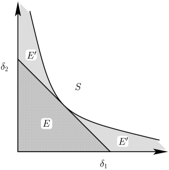
Figure 2: Gaussian states with the symmetric quadrature matrix ${\bf V}_{0}$ in Eq. (3) on the space of $\delta_{1}=n_{1}-|c_{1}|$ and $\delta_{2}=n_{2}-|c_{2}|$. Separable states are denoted by $S$ and entangled states by $E$ and $E^{\prime}$ with the boundary of $\delta_{1}\delta_{2}=1$. Further the two regions $E$ and $E^{\prime}$ are separated by the line $\delta_{1}+\delta_{2}=2$. The entanglement imposed on a state of the region $E^{\prime}$ may fail the entanglement test due to inefficient detection. However, the entangled state of the region $E$ is always found to be entangled regardless of the detection efficiency.

Consider the effect of the detection efficiency on the inseparability of the testing fields. Substituting $n_{i}^{\prime}$ and $c_{i}^{\prime}$ into Eq. (4) for inefficient detection, we find a state to be entangled when

$$(n^{\prime}-|c_{1}^{\prime}|)(n_{2}^{\prime}-|c_{2}^{\prime}|)=\eta^{2}(\delta_{1}\delta_{2}-\delta_{1}-\delta_{2}+1)$$

$$+\eta(\delta_{1}+\delta_{2}-2)+1<1.$$ (22)

Rearranging this equation, we can easily find that when the original testing field is characterized by $\delta_{1}+\delta_{2}<2$, it is always found to be entangled regardless of the detection efficiency unless the efficiency is zero. With use of (18) we find that a two-mode squeezed thermal field is extremely robust to the detection efficiency as an entangled two-mode squeezed state always passes the test of entanglement regardless of detection efficiency. Fig. 2 presents the sets of Gaussian states on the space of $\delta_{1}$ and $\delta_{2}$ where separable states with $\delta_{1}\delta_{2}\geq 1$ are denoted by $S$ and entangled states with $\delta_{1}\delta_{2}<1$ by $E+E^{\prime}$. All entangled states in the region $E$ with the condition, $\delta_{1}+\delta_{2}<2$, will violate the inequality (4) of the quadrature correlation unless the detection efficiency is zero while some entangled states in $E^{\prime}$ fail the test of entanglement.

It is also important to be able to tell a given state is pure. A degree of purity can be defined as $P=\mbox{Tr}\hat{\rho}^{2}$. When $P=1$ the state is pure. The purity of a two-mode Gaussian state can be performed using ideal homodyne detectors. For a Gaussian state of the quadrature matrix (3) the degree of purity $P=1/\sqrt{\det V}_{0}$. Noting that a vacuum is pure, the inequality of $P\leq 1$ can be written as

$$(\langle q_{1}^{2}\rangle^{2} - \langle q_{1}q_{2}\rangle^{2})(\langle p_{1}^{2}\rangle^{2}-\langle p_{1}p_{2}\rangle^{2})$$ (23)

$$\geq \left(\langle q_{1}^{2}\rangle^{2}-\langle q_{1}q_{2}\rangle^{2}\right)_{0}\left(\langle p_{1}^{2}\rangle^{2}-\langle p_{1}p_{2}\rangle^{2}\right)_{0}.$$

The equality implies that the testing fields are in the pure state (with the minimum uncertainty). For inefficient detectors, once their efficiencies are known as $\eta$, the purity may be deduced from the experimental data.

Reid and Drummond derived the inequality for the quantum correlation between two mode fields along the line with the Einstein, Podolsky and Rosen argument Reid ; Leuchs . They introduced the uncertainty $V_{1}$ ($V_{2}$) between the observable $q_{1}$ ($p_{1}$) in one mode and $q_{1}^{\prime}$ ($p_{1}^{\prime}$) inferred from the observation of the other mode. Quantum correlation may lead the product of the uncertainties to be less than the vacuum limit, resulting in the inequality of $V_{1}V_{2}<1$. In our notation this inequality can be written as

$$(n_{1}-|c_{1}|)(n_{2}-|c_{2}|)<\frac{n_{1}n_{2}}{(n_{1}+|c_{1}|)(n_{2}+|c_{2}|)}.$$ (24)

Note that the right hand side of the inequality is always less than unity. Thus, the inequality (24) is sufficient to satisfy our inseparable condition (see ( 4)). However, the converse statement does not hold in general.

We have proposed an experimental scheme to test the entanglement of a Gaussian field for the first time to the best of our knowledge. Our scheme is based on the inseparability criterion. The present scheme consists of balanced homodyne detectors which are well-established experimental tools to study quantum optics. We show that the entanglement imposed in a Gaussian state is measurable persistently against the detection efficiency if each mode has the roughly symmetric uncertainty over the phase space.

- (1) S. L. Braunstein and H. J. Kimble, Phys. Rev. Lett. 80, 869 (1998); A. Furusawa, J. L. Sørensen, S. L. Braunstein, C. A. Fuchs, H. J. Kimble, E. S. Polzik, Science 282, 706 (1998).
- (2) T. C. Ralph and P. K. Lam, Phys. Rev. Lett. 81, 5668 (1998).
- (3) S. Parker, S. Bose and M. Plenio, Phys. Rev. A61, 032305 (2000).
- (4) Ch. Silberhorn, P. K. Lam, O. Weiss, G. Koenig, N. Korolkova and G. Leuchs, Phys. Rev. Lett. 86, 4267 (2001).
- (5) R. Simon, Phys. Rev. Lett. 84, 2726 (2000).
- (6) L.-M. Duan, G. Giedke, J. I. Cirac and P. Zoller, Phys. Rev. Lett. 84, 2722 (2000).
- (7) J. Lee, M. S. Kim and H. Jeong, Phys. Rev. A62 032305 (2000).
- (8) K. Banaszek and K. Wódkiewicz, Phys. Rev. A55, 3117 (1997).
- (9) A. Kuzmich, I. A. Walmsley and L. Mandel, Phys. Rev. Lett. 85, 1349 (2000).
- (10) M. D. Reid and P. D. Drummond, Phys. Rev. Lett. 60, 2731 (1988); M. D. Reid, Phys. Rev. A40, 913 (1989).
- (11) M. S. Kim and B. C. Sanders, Phys. Rev. A53, 3694 (1996); M. S. Kim, W. Son, V. Bužek and P. L. Knight, Phys. Rev. A65, 032323 (2002).
- (12) C. W. Gardiner, Quantum Noise (Springer, Heidelberg, 1991).
- (13) R. Loudon and P. L. Knight, J. Mod. Opt. 34, 709 (1987).
- (14) R. A. Campos, B. E. A. Saleh, and M. C. Teich, Phys. Rev. A40, 1371 (1989).
- (15) S. M. Barnett and P. L. Knight, J. Mod. Opt. 34, 841 (1987).
- (16) H. P. Yuen and H. J. Shapiro, IEEE Trans. Inf. Theory 24, 657 (1978).
- (17) This can also be measured using a heterodyne detector.
- (18) U. Leonhardt and H. Paul, Phys. Rev. Lett. 72, 4086 (1994).