Laser driven atoms in half-cavities

Abstract

The behavior of a two level atom in a half-cavity, i.e. a cavity with one mirror, is studied within the framework of a one dimensional model with respect to spontaneous decay and resonance fluorescence. The system under consideration corresponds to the setup of a recently performed experiment [J. Eschner et. al., Nature 413, 495 (2001)] where the influence of a mirror on a fluorescing single atom was revealed. In the present work special attention is paid to a regime of large atom-mirror distances where intrinsic memory effects cannot be neglected anymore. This is done with the help of delay differential equations which contain, for small atom-mirror distances, the Markovian limit with effective level shifts and decay rates leading to the phenomenon of enhancement or inhibition of spontaneous decay. Several features are recovered beyond an effective Markovian treatment, appearing in experimental accessible quantities like intensity or emission spectra of the scattered light.

I Introduction

The change in the behavior of atoms when the structure of the “surrounding” field differs from that of free space is treated so far in innumerable works and is essentially the basic topic of cavity QED Berman (1994); Hinds (1991); Haroche (1990). Effects like modified decay rates of atoms in cavities were visible in various measurements Heinzen et al. (1987); Heinzen and Feld (1987); Jhe et al. (1987); Hulet et al. (1985); Goy et al. (1983); DeMartini et al. (1987). In this case, the atoms couple irreversibly to a large number of field modes and the problem can be treated within the framework of perturbation theory. This regime is therefore known as “low-Q” or perturbative cavity QED hin . Another area of high importance is its counterpart, the physics of “high-Q” cavities, where the atoms interact strongly only with one (or few) field mode(s). In this context, recent experiments include, e.g., the observation of atom trajectories in cavities storing merely one photon Hood et al. (2000); Pinkse et al. (2000). Furthermore, among other things, effects caused by the spatial structure of a field mode in a cavity were demonstrated Mundt et al. ; Guthöhrlein et al. (2001). High-Q cavities serve also as a testing ground for fundamental quantum mechanical effects like entanglement or decoherence Raimond et al. (2001); wal .

Besides some considerations on the spontaneous decay of an excited two-level atom we will mainly focus in this paper on the problem of resonance fluorescence in a half-cavity, i.e. a cavity with one mirror, where we pay special attention to the position dependence of the atomic dynamics. To this end we will particularly consider a physical system which essentially coincides with the setup of an recently performed experiment Eschner et al. (2001). Here, the radiation which is emitted by a laser cooled ion stored in Paul trap is partly collimated by a lens and reflected back by a mirror to the atom. The intensity of the scattered light was measured as a function of the mirror position leading to an oscillatory behavior of the photon counting rate, proving the existence of inhibited and enhanced spontaneous emission effects. In this case, where the atom is relatively close to the mirror, the observed effects can in principal explained by introducing some effective modified (position dependent) spontaneous emission rates and level shifts. This could be done since the time the light needs to bounce back and forth between the atom and the mirror could be set essentially to zero (Markovian limit). The situation is more complicated when the distance between the atom and the mirror is large.

In this paper we will, among other things, particularly consider this case and it turns out that the dynamics of the atom can be described generally in terms of non-Markovian (delay-differential) equations. As we will see, the distance between the atom and the mirror influences the atomic behavior essentially on two scales: On the one hand, on a large scale, i.e. whether the atom is located far away from the mirror or very close to the mirror. This scale can be measured essentially by a dimensionless quantity $\Gamma_{0}\tau$ where $\Gamma_{0}$ is given by the width of the field spectrum (in case of vanishing laser intensity it is simply the atomic spontaneous emission rate) and the time $\tau$ the light needs for a round trip between atom and mirror. On the other hand, the atomic behavior varies also if the distance is changed on the scale of an optical wavelength given by $\omega_{L}\tau$. For example in case of a small atom-mirror distance ($\Gamma_{0}\tau\ll 1$) the equations of motions become approximately Markovian and the well-known phenomenon of enhanced or inhibited spontaneous emission (depending on $\omega_{L}\tau$), can be recovered. Thus, it is possible to describe the system by introducing effective spontaneous emission rates and level shifts. In general, however, the retardation of the time argument in the equations of motion cannot be neglected. We will not consider in this paper effects arising in the case of extremely small distances, i.e. of the order of wavelengths or smaller, between the atom and the mirror Milonni (1994); Hinds (1991); hin ; Meschede et al. (1990); Hinds and Sandoghdar (1991).

In connection with cavity QED, in the broadest sense, the above mentioned delay-differential equations appeared already in some works. These include for example the analytical treatments of Milonni et al. Milonni et al. (1983) in which a single excited quantum system coupled to an infinite set of equally spaced discrete levels was considered, a system which reminds of an atom in a cavity but without taking into account some position depending effects. The latter problem was discussed in the framework of a one-dimensional model by Cook and Milonni Cook and Milonni (1987) in case of an excited atom in front of a partially reflecting wall (modeled as a collection of two-level atoms) and in a Fabry-Perot resonator. This treatment is closely related to our discussion of pure spontaneous decay since we will recover the same equation of motion. Another treatment of this problem was given by Feng and Ujihara Feng and Ujihara (1990) by using an appropriate set of mode functions in order to account for non-perfect mirror reflectivities. Dung and Ujihara Dung and Ujihara (1999) finally examined an atom in a three-dimensional Fabry-Perot resonator. Although a delay differential equation was not explicitly formulated, retardation effects in the interaction of two atoms were also discussed in Milonni and Knight (1974, 1975). A partly numerical examination of an atom inside a spherical cavity was given by Parker and Stroud Parker and C. R. Stroud Jr. (1987). Numerical examinations include furthermore the work of Gießen et al.Gießen et al. (1996) and Bužek et al. Bužek et al. (1999) both treating an atom in a (one-dimensional) cavity whereas the latter also investigates the presence of material media. The mentioned works have in common that recurrences of the atomic population take place for large dimensions of the cavity which is due to one-photon wave packets bouncing back and forth between the cavity walls. However, there is always only one excitation contained in the system making the problem accessible for analytical considerations.

In case of a (near-)resonantly driven atom the dynamics of the system is more complicated since the number of excitations increase continuously. The scattered radiation will be reflected by the mirror and re-interact with its own source, the atom. This situation reminds us of a feedback problem Wiseman (1994); Wiseman and Milburn (1994) where mostly the assumption of a negligible feedback time delay is made. However, the situation of large atom-mirror distances would correspond to a non-Markovian feedback Giovannetti et al. (1999); Wang et al. (2001).

This article is structured as follows. In Sec. II we will reconsider the problem of pure spontaneous decay of an excited atom in the presence of a mirror while in Sec. III a continuous laser excitation of the atom is incorporated to our examination. We will discuss several limits including low and higher laser intensities and small distances between the atom and the mirror. Finally, a summary is given in Sec. IV and cumbersome formulas and calculations are moved to appendices.

II Spontaneous emission

In this section we will investigate the spontaneous emission of an atom at rest in the presence of a mirror initially prepared in the excited state. We will derive a non-Markovian equation of motion for this system. Although this derivation is related to the calculations in Cook and Milonni (1987) it will be discussed here, not only to introduce our notation but also to present new, entirely analytical results, also with respect to spectral properties of the emitted light. Furthermore it will turn out that some calculation methods can be transfered and some features of this system are recovered when we include laser excitation in our considerations.

II.1 The model

As already mentioned we examine an initially excited two-level atom with transition frequency $\omega_{0}$ in the presence of a finite size mirror where the light emitted in a certain solid angle fraction $\varepsilon$ is reflected back to the atom. This is achieved by a lens which collimates the radiation before it is reflected Eschner et al. (2001). The remaining emission is not affected by the mirror. Thus, it is reasonable to consider the coupling of the atom to two reservoirs (or “channels”) consisting of one-dimensional fields with standing wave field modes and running wave field modes, respectively (see Fig. 1), i.e. the Hamiltonian in rotating wave approximation reads

$$H=H_{0} - d\big{(}E^{\dagger}_{1}(L)\sigma_{-}+\sigma_{+}E_{1}(L)\big{)}$$ (1)

$$- d\big{(}E^{\dagger}_{2}(0)\sigma_{-}+\sigma_{+}E_{2}(0)\big{)}$$

with

$$H_{0}=\hbar\omega_{0}\sigma_{+}\sigma_{-}+\int\text{d}k\,\hbar\omega_{k}a_{k}^{\dagger}a_{k}+\int\text{d}k\,\hbar\omega_{k}b_{k}^{\dagger}b_{k},$$

$$E_{1}(z)=\text{i}\int\text{d}k\,\alpha_{k}\sin(kz)a_{k},\quad k>0,$$

$$E_{2}(x)=\text{i}\int\text{d}k\,\beta_{k}\text{e}^{\text{i}kx}b_{k},\quad k\in\mathbb{R},$$ (2)

and $\omega_{k}=|k|c$. In contrast to a cavity, here, the mode density of the mirror channel is continuous since only one boundary condition has to be fulfilled. The operators $\sigma_{+},\,\sigma_{-}$ are the usual raising and lowering operators of a two-level system with upper level $|e\rangle$ and ground state $|g\rangle$, $\sigma_{+}=|e\rangle\langle g|$, $\sigma_{-}=|g\rangle\langle e|$, and $a_{k}^{\dagger},\,b_{k}^{\dagger},\,a_{k},\,b_{k}$ are creation and annihilation operators of a photon in the $k$th mode of the different environments. The dipole matrix element $d$ is assumed to be real and for the sake of simplicity we suppress the vectorial character of $d$ and $E$. The exact form of the factors $\alpha_{k}$ and $\beta_{k}$ is of no importance here, we merely assume that they are approximately constant in a frequency range of relevance (usually they have a frequency dependence $\alpha_{k}\sim\sqrt{\omega_{k}}$ and $\beta_{k}\sim\sqrt{\nu_{k}}$). In order to investigate the dynamics of the system we make the Wigner-Weisskopf type ansatz

$$|\psi(t)\rangle= b_{e}(t)|e,\{0\}_{1},\{0\}_{2}\rangle$$ (3)

$$+ \int\text{d}k\,b_{g,k}^{1}(t)|g,\{k\}_{1},\{0\}_{2}\rangle$$

$$+ \int\text{d}k\,b_{g,k}^{2}(t)|g,\{0\}_{1},\{k\}_{2}\rangle,$$

where $|\{0\}\rangle$ denotes the vacuum state of the radiation field and $|\{k\}\rangle$ the state with exactly one photon in mode $k$. We will consider here an initially excited atom in the absence of any photon, i.e. $b_{e}(0)=1$ and $b_{g,k}^{j}(0)=0$. In contrast to the notation in Eq. (3), in the following the amplitudes are always taken in a rotating frame, i.e. we make the substitutions $b_{e}(t)\rightarrow b_{e}(t)\text{e}^{-\text{i}\omega_{0}t}$ and $b_{g,k}^{j}(t)\rightarrow b_{g,k}^{j}(t)\text{e}^{-\text{i}\omega_{k}t}$ .

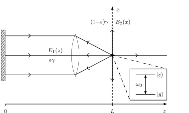
Figure 1: Sketch of the physical system under consideration. The radiation emitted by a two-level atom is partly reflected (via a lens) back to the atom which is modeled by an atom coupled to two one-dimensional channels with a different mode structure (running and standing wave modes, respectively).

With the help of the “essential states” contained in the above ansatz it is possible to write down a closed set of equations of motion for the amplitudes which take the form

$$\dot{b}_{e}(t)=-\int\text{d}k\,g_{k}\sin(kL)\text{e}^{-\text{i}(\omega_{k}-\omega_{0})t}b_{g,k}^{1}(t)$$

$$\qquad\quad-\int\text{d}k\,h_{k}\text{e}^{-\text{i}(\omega_{k}-\omega_{0})t}b_{g,k}^{2}(t),$$ (4a)

$$\dot{b}_{g,k}^{1}(t)=g_{k}\sin(kL)\text{e}^{\text{i}(\omega_{k}-\omega_{0})t}b_{e}(t),$$ (4b)

$$\dot{b}_{g,k}^{2}(t)=h_{k}\text{e}^{\text{i}(\omega_{k}-\omega_{0})t}b_{e}(t)$$ (4c)

with $g_{k}\equiv\alpha_{k}d/\hbar$ and $h_{k}\equiv\beta_{k}d/\hbar$.

By formally integrating the latter two equations and inserting them into the first one we get

$$\dot{b}_{e}(t) = -\int_{0}^{t}\text{d}t^{\prime}\,b_{e}(t^{\prime})\int\text{d}k\,g_{k}^{2}\sin^{2}(kL)\text{e}^{\text{i}(\omega_{k}-\omega_{0})(t^{\prime}-t)}$$ (5)

$$-\int_{0}^{t}\text{d}t^{\prime}\,b_{e}(t^{\prime})\int\text{d}k\,h_{k}^{2}\text{e}^{\text{i}(\omega_{k}-\omega_{0})(t^{\prime}-t)}$$

$$= -\gamma\int_{0}^{t}\text{d}t\,b_{e}(t^{\prime})\delta(t^{\prime}-t)\text{e}^{-\text{i}\omega_{0}(t^{\prime}-t)}$$

$$+\varepsilon\frac{\gamma}{2}\int_{0}^{t}\text{d}t^{\prime}\,b_{e}(t^{\prime})[\delta(t^{\prime}-t+\tau)$$

$$\hskip 54.2025pt+\delta(t^{\prime}-t-\tau)]\text{e}^{-\text{i}\omega_{0}(t^{\prime}-t)}.$$

Here, we introduced the free space spontaneous decay rate $\gamma$ which is split up into a part $\varepsilon\gamma\equiv\pi g_{k_{0}}^{2}/c$ and $(1-\varepsilon)\gamma\equiv 4\pi h_{k_{0}}^{2}/c$, corresponding to the coupling of the atom to the first and second channel. The quantity $\varepsilon$ is the solid angle fraction which is covered by the lens since it characterizes the fraction of radiation which is reflected. In the above equations we also introduced the time $\tau\equiv 2L/c$ the light needs for the distance atom-mirror-atom. Furthermore, in the first step of (5), a Wigner-Weisskopf type approximation was made based on the well-known fact that the relative variation of $g_{k}^{2},\,h_{k}^{2}$($\sim\omega$) is very slow in the domain where the double integration in the first line of (5) lead to appreciable values. Diverging terms connected with level shifts are omitted. It should be stressed here that in this paper only distances between the atom and the mirror are considered which are much larger than an optical wavelength, i.e. $\omega_{0}\tau\gg 1$ which is in an optical frequency domain already the case for, say, a millimeter.

Eq. (5) yields finally the delay differential equation

$$\dot{b}_{e}(t)=-\frac{\gamma}{2}b_{e}(t)+\varepsilon\frac{\gamma}{2}\text{e}^{\text{i}\omega_{0}\tau}b_{e}(t-\tau)\Theta(t-\tau),$$ (6)

where $\Theta(t)$ is the Heaviside step function. The first term on the right hand side of this equation corresponds to the usual free space exponential decay while the second term represents the effect of the reflected radiation on the atom which was emitted at time $\tau$ before it interacts again with the atom. Thus, the retarded argument of the excited state amplitude directly indicates the memory effects which are inherent in the system. Furthermore, the second term is weighted with the factor $\varepsilon$ revealing that only a fraction of the emitted light is reflected.

Eq. (6) is a delay-differential equation Driver (1977) and since we will encounter in Sec. III.2.2 and Sec. III.2.3 some more complicated equations of this type we move a further discussion of some general properties of equations of this kind to these sections.

II.2 Discussion

Using Laplace transformation and geometric series expansion Eq. (6) can easily be solved and one obtains

$$b_{e}(t)=\sum_{n=0}^{\infty}\frac{(\varepsilon\gamma/2)^{n}}{n!}\text{e}^{\text{i}\omega_{0}n\tau}\text{e}^{-\frac{\gamma}{2}(t-n\tau)}(t-n\tau)^{n}\Theta(t-n\tau).$$ (7)

It should be mentioned that this expression can also be obtained by a direct Laplace transformation of the Schrödinger equation (4) Milonni and Knight (1974).

The above solution reveals that the systems dynamics has a “step” character which can be seen most easily if one divides the time axis into intervals of length $\tau$. For $t\in[0,\tau]$ the sum consists only of one term, $\exp(-\gamma\tau/2)$, which coincides with the free space behavior of a decaying atom. The physical reason for that is that the atom requires at least the time the light needs to get from the atom to the mirror and back to the atom again in order to “see” the mirror. For $t\in[\tau,2\tau]$ the amplitude consists of two terms,

$$b_{e}(t)=\text{e}^{-\frac{\gamma}{2}t}+\varepsilon\frac{\gamma}{2}\text{e}^{\text{i}\omega_{0}\tau}\text{e}^{-\frac{\gamma}{2}(t-\tau)}(t-\tau),$$ (8)

giving rise to an interference term in the probability of finding the atom in the excited state. The second term is due to the emitted radiation reflected back to the atom. The light the atom emits right now arrives the atom again at the beginning of the third time interval where the sum in (7) includes a further term and so on.

The role of the interference terms in the excited state probabilities strongly depends on the distance between the atom and the mirror which can be measured by the quantity $\gamma\tau$. If we consider again the second time interval it is easy to see that that the interference term is of order $\gamma\tau$ while a further term is of order $(\gamma\tau)^{2}$ which can be neglected for $\gamma\tau\ll 1$ (small distance). Hence we get the expression

$$|b_{e}(t)|^{2}\approx\text{e}^{-\gamma t}(1+\varepsilon\gamma(t-\tau)\cos(\omega_{0}\tau)),\quad t\in[\tau,2\tau],$$ (9)

where we guess the beginning of an exponential series. The examination of the dynamics in this limit for larger times based on Eq.(7) is relatively complicated. It is more convenient to return to the delay differential equation (6). Since we are working in a rotating frame the amplitude $b_{e}(t)$ varies slowly on a time scale given by $1/\gamma$. Thus, in the limit $\gamma\tau\ll 1$ we can make the approximation $\tau\rightarrow+0$ in the argument of $b_{e}$ in the second term on the right hand side of Eq. (6) and obtain the Markovian equation

$$\dot{b}_{e}(t)\approx\begin{cases}-\frac{\gamma}{2}b_{e}(t)&;\,t\leq\tau\\ -\frac{\gamma}{2}(1-\varepsilon\text{e}^{\text{i}\omega_{0}\tau})b_{e}(t)&;\,t>\tau.\end{cases}$$ (10)

This leads to the excited state probability

$$|b_{e}(t)|^{2}\approx\begin{cases}\text{e}^{-\gamma t}&;\,t\leq\tau\\ \text{e}^{-\gamma\tau}\text{e}^{-\tilde{\gamma}(t-\tau)}&;\,t>\tau\end{cases}$$ (11)

with $\tilde{\gamma}=\gamma(1-\varepsilon\cos(\omega_{0}\tau))$. The upper state population based on the exact amplitude (7) in this limit is shown in Fig. 2. The behavior of the curves coincide almost perfectly with the predictions of Eq. (11): After a period of length $\tau$ there is an enhancement or inhibition of spontaneous decay depending on the factor $1-\varepsilon\cos(\omega_{0}\tau)$ which corresponds to the amplitude of a standing wave mode $\sin{(k_{0}z)}$ at the position of the atom: In a node of the standing wave, spontaneous decay is inhibited while in an antinode it is enhanced.

Figure 2: Upper state population of an atom close to the mirror for different exact positions, i.e. $\omega_{0}\tau=2n\pi$ (node) and $\omega_{0}\tau=(2n+1)\pi$ (antinode). The remaining parameters are $\varepsilon=0.4$, $\gamma\tau=0.4$. Also indicated is the corresponding free space solution ($\varepsilon=0$).

To get a more physical insight in this behavior the intensity of the electric field $E_{1}$ which is reflected by the mirror depending on space and time is shown in Fig. 3. The derivation of an analytical expression for $\langle E_{1}^{\dagger}(z,t)E_{1}(z,t)\rangle$ can be found in Appendix A. In a realistic situation with regard to the setup considered here the frequency of the oscillations which can be seen in Fig. 3 (and also in Fig. 5) would be significantly higher than indicated in these figures. However, for the sake of visibility, a rather small frequency is chosen here.

Figure 3: Intensity of the field at different points of time for the parameters of Fig. 2. The atom is located at a node (i.e. $\omega_{0}\tau=2n\pi$) at $z=L$.

Due to the small distance between the atom (located at $z=L$) and the mirror (located at $z=0$) the reflected light has the possibility to interfere with the radiation which is still emitted by the atom leading to a standing wave pattern of the form $\sim\sin^{2}(k_{0}z)$ that has, in case of the example shown in Fig. 3, a node at the position of the atom, i.e. a zero electric field. Due to this fact, further emission of radiation in this channel is suppressed. Another interesting feature with respect to Fig. 3 is that the amplitude of the standing wave decreases for $\varepsilon<1$ with increasing time whereas the energy escapes in the other channel. The situation is reminiscent of a cavity where the atom acts like a partially transmitting mirror.

In the limit of large distances between atom and mirror (i.e. $\gamma\tau\gg 1$) the sum (7) is dominated by the term with the highest power of $\gamma\tau$. Hence, we get in a time interval $[m\tau,(m+1)\tau]$

$$|b_{e}(t)|^{2}\approx\left(\frac{(\varepsilon\gamma/2)^{m}}{m!}\right)^{2}\text{e}^{-\gamma(t-m\tau)}(t-m\tau)^{2m}.$$ (12)

We see that the atom is partially reexcited by the radiation which it has emitted before and that the exact position (node or antinode) is not significant. This is illustrated in Fig. 5 and Fig. 5 where we plot again the exact solution for the excited state amplitude and the field intensity.

Figure 4: Upper state population of an atom far away from the mirror and $\omega_{0}\tau=2n\pi$. The remaining parameters are $\varepsilon=0.4$, $\gamma\tau=10$. The inset is a vertical magnification.

Figure 5: Intensity of the field at different points of time for the parameters of Fig. 5. The atom is located again at $z=L$ while the inset is a vertical magnification.

The atom is placed in a node of the standing wave and the inset in Fig. 5 is a magnification in vertical direction of that part. We see that interference between outgoing and incoming radiation is much weaker than in Fig. 3.

In this context it is also interesting to take a look at the spectrum of the emitted light (here this means the probability of finding a photon of frequency $\omega$ in the long time limit). This can easily be calculated by integrating Eq. (4b) and Eq. (4c) and using Eq. (7) which leads to

$$b_{g}^{j}(\omega,t) = \frac{A_{j}(\omega)}{\frac{\gamma}{2}+\text{i}(\omega_{0}-\omega)}\sum_{n=0}^{\infty}\frac{(\varepsilon\gamma/2)^{n}}{n!}\text{e}^{\text{i}\omega n\tau}(t-n\tau)^{n}$$

$$\quad\times G_{n}[-({\textstyle\frac{\gamma}{2}}+\text{i}(\omega_{0}-\omega))(t-n\tau)]\Theta(t-n\tau)$$

with

$$G_{n}[s]\equiv\sideset{{}_{1}}{{}_{1}}{\operatorname{F}}[n,n+1;s]-\text{e}^{s},$$ (14)

where $\sideset{{}_{1}}{{}_{1}}{\operatorname{F}}[n,m;x]$ is the confluent hypergeometric function and

$$A_{j}(\omega)\equiv\begin{cases}\sqrt{\frac{\varepsilon\gamma}{\pi}}\sin(\omega\tau/2),\quad j=1\\ \sqrt{\frac{(1-\varepsilon)\gamma}{2\pi}},\quad j=2.\end{cases}$$ (15)

The transient photon population of the second channel in case of a relatively large atom-mirror distance for an atom placed in an antinode of the resonant standing wave field mode is shown in Fig. 6.

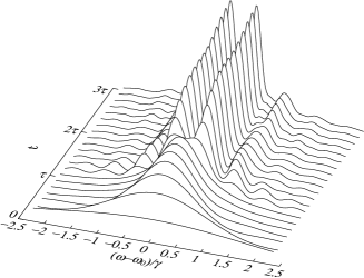
Figure 6: Transient photon population in channel $2$ depending on frequency and time for a large distance between the atom (placed at an antinode, i.e.  $\omega_{0}\tau=(2n+1)\pi$) and the mirror. Further parameters are $\varepsilon=0.4$ and $\gamma\tau=10$.

In the long time limit the spectra take the form

$$|b_{g}^{j}(\omega)|^{2}=\frac{A_{j}^{2}(\omega)}{\frac{\gamma^{2}}{4}(1-\varepsilon\cos(\omega\tau))^{2}+\left(\varepsilon\frac{\gamma}{2}\sin(\omega\tau)+\omega-\omega_{0}\right)^{2}}.$$ (16)

Fig. 7 shows the steady state photon population of the channel parallel to the mirror for different atomic positions.

Figure 7: Frequency dependent steady state photon population in case of a large distance between the atom and the mirror. The exact position of the atom is a node ($\omega_{0}\tau=2n\pi$) or an antinode ($\omega_{0}\tau=(2n+1)\pi$), respectively ($\varepsilon=0.4$, $\gamma\tau=10$).

The frequencies of the local minima in Fig. 6 and Fig. 7 coincide approximately with the frequencies of those standing wave modes which have an antinode at the position of the atom. This means that the photon distribution in the second channel, which has initially roughly the shape of a Lorentzian (at the end of the time interval $[0,\tau]$, see Fig. 6), is affected by the back reflected light in the first channel. Here, the radiation components with the mentioned frequencies have a higher probability to be reabsorbed and emitted again (perhaps in modes of other frequencies). This leads to a lower population of these modes.

If the atom is very close to the mirror we recognize that the differential equation Eq. (10) contains the complex phase $\text{e}^{\text{i}\omega_{0}\tau}$, where the imaginary part of this factor can be interpreted as a level shift. This has consequences for the spectrum which takes in this limit the form

$$|b_{g}^{2}(\omega)|^{2}\sim\frac{1}{\tilde{\gamma}^{2}/4+(\omega-\tilde{\omega}_{0})^{2}},$$ (17)

where $\tilde{\gamma}$ is defined in Eq. (10) and

$$\tilde{\omega}_{0}\equiv\omega_{0}-\varepsilon\frac{\gamma}{2}\sin(\omega_{0}\tau).$$ (18)

This expression can be derived with the help of Eq. (10) (where we neglect the small contribution arising from the first time interval $[0,\tau]$) or with Eq. (16) using the fact that for $\gamma\tau\ll 1$ the trigonometric functions in the denominator of Eq. (16) vary very slowly on a frequency scale $\gamma$. The form of this spectrum illustrates first of all again the behavior shown in Fig. 2, i.e. the width of the Lorentzian is larger or smaller depending whether the atom is placed in an antinode or a node of a standing wave $\sin(k_{0}z)$. On the other hand the maximum of the function is shifted according to the imaginary part of the mentioned phase. The physical interpretation of this shift is based on the fact that the atom interacts with its own radiation. It corresponds to the energy of the atomic dipole in the reflected electric field hin ; Hinds (1991); Meschede et al. (1990); Hinds and Sandoghdar (1991).

III Laser excitation

The system discussed in the previous section was amenable to an exact analytical treatment since the equations of motion decoupled by using a Wigner-Weisskopf (or Markov)-type approximation. This reduced the problem essentially to the solution of one equation describing only the atomic dynamics. This was possible because the system contained merely one excitation. The dynamics of the atom-field system becomes more complicated when we include a continuous laser excitation of the atom. The number of photons scattered by the atom into the two channels will permanently increase and a part of them will be reflected back, interacting again with the atom in addition to the laser light. The atom starts now to emit a different kind of radiation which again returns to the atom after some time and so on. Thus we expect that an electric field is constituted with a complex structure. The behavior of the system reminds us of that of a cascaded quantum system Carmichael (1993); Gardiner (1993); Kochan and Carmichael (1994); Gardiner and Parkins (1994); Gardiner and Zoller (2000), a formalism which deals with systems driven by non-classical types of light and which was applied in the theory of Markovian feedback Wiseman and Milburn (1994).

The non-Markovian feedback contained in the system discussed here makes it difficult to solve the problem in an exact analytical way since it is not possible to establish a closed set of equations describing the dynamics of the atom as in the theory of Markovian resonance fluorescence. Thus we are restricted to approximative methods in the following sections.

III.1 Perturbation theory

Using the results of Sec. II we will, as a starting point, examine the influence of the laser for low intensities within the framework of a time dependent perturbation theory. Here, as well as in the following sections, the effect of the laser is included in our considerations with the help of the standard semi-classical model for atom-laser interaction in rotating wave approximation, i.e. the new Hamiltonian reads

$$H_{L}=H+V(t),$$ (19)

with

$$V(t)=-\hbar\frac{\Omega_{0}}{2}(\text{e}^{\text{i}\omega_{L}t}\sigma_{-}+\text{e}^{-\text{i}\omega_{L}t}\sigma_{+})$$ (20)

and laser- and Rabi-frequency $\omega_{L}$ and $\Omega_{0}$, respectively. Taking the ground state of the atom-field system as initial state we get in first order perturbation theory (assuming a weak laser intensity) the excited state amplitude in a rotating frame

$$b_{e}^{L}(t) = \text{e}^{\text{i}\omega_{L}t}\frac{1}{\text{i}\hbar}\int_{0}^{t}\text{d}t^{\prime}\,\langle E|\text{e}^{-\text{i}H(t-t^{\prime})/\hbar}V(t^{\prime})\text{e}^{\text{i}Ht/\hbar}|G\rangle$$ (21)

$$= \text{i}\frac{\Omega_{0}}{2}\int_{0}^{t}\text{d}t^{\prime}\,\text{e}^{-\text{i}\Delta t^{\prime}}b_{e}(t^{\prime}),$$

with $|E\rangle\equiv|e,\{0\}_{1},\{0\}_{2}\rangle$, $|G\rangle\equiv|g,\{0\}_{1},\{0\}_{2}\rangle$ and laser detuning $\Delta\equiv\omega_{0}-\omega_{L}$. The above expression is essentially equivalent to the one-photon amplitude of Sec. II.2 if the laser frequency $\omega_{L}$ is replaced by $\omega$. Thus, we immediately get

$$b_{e}^{L}(t) = \frac{\text{i}\Omega_{0}}{\gamma+2\text{i}\Delta}\sum_{n=0}^{\infty}\frac{(\varepsilon\gamma/2)^{n}}{n!}\text{e}^{\text{i}\omega_{L}n\tau}(t-n\tau)^{n}$$ (22)

$$\quad\times G_{n}[-({\textstyle\frac{\gamma}{2}}+\text{i}\Delta)(t-n\tau)]\Theta(t-n\tau).$$

Figure 8: Upper state population in case of an atom far away from the mirror ($\gamma\tau=20$, $\varepsilon=0.4$) and weak laser excitation ($\Omega_{0}=0.05\gamma$) for an atom placed in an antinode (dashed line, $\omega_{L}\tau=(2n+1)\pi$, $\Delta=0$), in a node (solid line, $\omega_{L}\tau=2n\pi$, $\Delta=0$) and at a “slope” (dashed-dotted line, $\omega_{L}\tau=(2n-\frac{1}{2})\pi$, $\Delta=-0.2\gamma$).

Examples for the excited state amplitude are shown in Fig. 8 for different positions of the atom whereas the overall distance of the atom and the mirror is chosen to be quite large. The form of the curves has a direct interpretation. Since for low laser intensities coherent light scattering dominates the reflected radiation leads to a lower or higher “driving force” depending on the position of the atom. The system has similarities to an atom which is driven by two lasers where the phase difference is controlled by the distance between atom and mirror. Actually the superimposed intensity of the lasers changes after each round trip of the light which leads to a transient upper state population as shown in Fig. 8. For example, if the atom is placed in a node the laser interferes always constructively with the “reflected” laser beam giving rise to a higher population in a time interval $[n\tau,(n+1)\tau]$ compared to the preceding one. This point will be further developed in the Sec. (III.2.2) where we reconsider the limit of low laser intensities.

The steady state population obtained from Eq. (21) is given by

$$\underset{t\rightarrow\infty}{\lim}|b_{e}^{L}(t)|^{2}=\frac{\Omega_{0}^{2}}{{\tilde{\gamma}_{L}}^{2}+4{\tilde{\Delta}}^{2}}$$ (23)

with modified decay rate and detuning

$$\tilde{\gamma}_{L} = \gamma(1-\varepsilon\cos(\omega_{L}\tau),$$ (24a)

$$\tilde{\Delta} = \Delta-\varepsilon\frac{\gamma}{2}\sin(\omega_{L}\tau).$$ (24b)

The situation is similar to the Markovian limit of the previous section, i.e. we have a pronounced dependence of the atomic dynamics on the exact position of the atom (e.g. node or antinode of a standing wave of the laser frequency $\sin(k_{L}z)$). The difference is that this fact still holds in case of large atom-mirror distances. In the sense of Figs. (3) and (5) this is due to the fact that the interference ability of outgoing and reflected light does not depend on the distance since the laser provides a continuous scattered light field.

A further quantity which is of interest in this context is the the second order intensity correlation function,

$$\langle E^{\dagger}_{j}(t)E^{\dagger}_{j}(t+T)E_{j}(t+T)E_{j}(t)\rangle=|\alpha_{j}|^{4}G^{(2)}_{j}(t,t+T),$$ (25)

where the index $j=1,2$ indicates which channel is considered and $\alpha_{j}\equiv(\delta_{j2}-\varepsilon)\gamma\hbar/(2d)$. Expressions for the electric field operators are given in Appendix A. This correlation function corresponds to the probability of detecting a photon at time $t+T$ on condition that at time $t$ a first one was detected (see e.g. Glauber (1963)).

Assuming that the detectors are arranged as in Fig. 11 we have in the channel parallel to the mirror

$$G^{(2)}_{2}(t,t+T) = \langle\sigma_{+}(t)\sigma_{+}(t+T)\sigma_{-}(t+T)\sigma_{-}(t)\rangle$$ (26)

$$= \|\sigma_{-}U(t+T,t)\sigma_{-}U(t,0)|G\rangle\|^{2}.$$

By calculating the time evolution $U$ in first order perturbation theory we obtain

$$G^{(2)}_{2}(t,t+T)=|b_{e}^{L}(t)|^{2}|b_{e}^{L}(T)|^{2},$$ (27)

or in the long time limit

$$\underset{t\rightarrow\infty}{\lim}G^{(2)}_{2}(t,t+T)=\frac{\Omega_{0}^{2}}{{\tilde{\gamma}_{L}}^{2}+4{\tilde{\Delta}}^{2}}|b_{e}^{L}(T)|^{2},$$ (28)

i.e. for $\gamma\tau\gg 1$ we have a behavior as shown in Fig. 8. This can be interpreted as follows. After the detection of the first photon the atom is in its ground state and has to be re-excited again before it is able to emit a second photon (antibunching). The radiation which is emitted now (the second photon) is split up into a part emitted into channel $2$ and a part which is emitted into channel $1$. If $T<\tau$ the light which is (or will be) reflected in channel $1$ is not able to reach the atom before the photon detection in channel $2$. Thus, we encounter, except for a constant factor, the same behavior as in free space. However, if there is enough time for the radiation in channel $1$ to make a complete round trip, it is able to re-interact with the atom (in addition to the laser), which leads to a higher or lower emission probability in channel $2$.

Figure 9: The four contributions to the second order intensity correlation function and the corresponding space-time diagrams. The correlation function is the squared norm of the sum of these vectors. The atom is located at $L$, the detector at $z_{0}$ and the distance between them is denoted as $d_{0}$. It is assumed that the detection of the first and second atom takes place at a time $t$ and $t+T$, respectively. The $\bullet$-symbol indicates the time of emission in the past relative to the detection times. The ordering of the operators in d) changes if $T$ becomes smaller than $\tau$ (dotted line).

An expression for $G^{(2)}_{1}(t,t+T)$ is derived in Appendix A where we assumed again a detector arrangement as in Fig. 11, i.e. the atom is located in between the mirror and the detector. It is written as the norm of a sum of four states. These four contributions (in a non-rotating frame) are shown in Figs. 9a)-9d) where each of these terms is connected to a different path leading to a coincidence detection at time $t$ and $t+T$. The back action of the light on the atom is included in the dynamics of the time dependent operators. In principle the light has two possibilities to get to the detector: Either it takes the direct way or the indirect way via the mirror which leads to four possibilities for a two-photon detection amplitude indicated by the space-time diagrams in Fig. 9. For the sake of clarity the arbitrary distance between detector and atom, $d_{0}$, is not set to zero which is also indicated in the time arguments of the operators. For calculations however, we will always set $d_{0}=0$. The time arguments of the operators coincide with the emission time in the past relative to $t$ and $t+T$, respectively. Note, that a possibility which includes a reflection gives rise to a negative sign and that the ordering of the operators in Fig. 9d) depends on the length of the delay interval $T$. The four contributions will interfere since they remain indistinguishable when a coincidence signal occurs.

For weak laser intensities these quantities can be calculated using first order perturbation theory in a similar way as it was done in the derivation of Eq. (27) which leads to an expression of fourth order in $\Omega_{0}$,

$$G_{1}^{(2)}(t,t+T)=| b_{e}^{L}(T)b_{e}^{L}(t)+\text{e}^{2\text{i}\omega_{L}\tau}b_{e}^{L}(T)b_{e}^{L}(t-\tau)$$

$$-\text{e}^{\text{i}\omega_{L}\tau}b_{e}^{L}(T+\tau)b_{e}^{L}(t-\tau)$$

$$-\text{e}^{\text{i}\omega_{L}\tau}b_{e}^{L}(|T-\tau|)b_{e}^{L}(t+s)|^{2},$$ (29)

where $s=0$ if $T>\tau$ and $s=T-\tau$ if $T\leq\tau$. We omitted step functions in this expression. In case of negative arguments the corresponding quantities have to be set to zero. Recall that these amplitudes are written in a rotating frame. In the long time limit we have

$$\underset{t\rightarrow\infty}{\lim}G_{1}^{(2)}(t,t+T)=\frac{\Omega_{0}^{2}}{{\tilde{\gamma}_{L}}^{2}+4{\tilde{\Delta}}^{2}}$$

$$\qquad\times|2b_{e}^{L}(T)\cos(\omega_{L}\tau)-b_{e}^{L}(T+\tau)-b_{e}^{L}(|T-\tau|)|^{2}.$$ (30)

Figure 10: Second order intensity correlation function for a weakly driven atom ($\Omega_{0}=0.05\gamma$, $\varepsilon=0.4$) located at an antinode ($\omega_{L}\tau=(2n+1)\pi$), a “slope” ($\omega_{L}\tau=(2n-\frac{1}{2})\pi$) and a node ($\omega_{L}\tau=2n\pi$) of the standing wave $\sin(k_{L}z)$. The overall distance between the atom and the mirror is assumed to be quite large ($\gamma\tau=20$) while the laser is tuned to exact resonance ($\Delta=0$).

This function is shown in Fig. 10 for a relatively large atom-mirror distance. Several features are visible: First of all $G_{1}^{(2)}$ is not zero for $T=0$. Indeed, diagram a) and diagram b) do not contribute to the detection probability in this case which reflects the fact that after an emission process the atom is in its ground state and the probability amplitude that it immediately emits a second photon is zero. On the other hand, if the first photon is detected (and the atom is in the lower state) there is still the possibility that there is radiation around caused by a prior emission process which is represented by the remaining diagrams. Due to this fact the value of $G^{(2)}_{1}$ for $T=0$ differs from those for larger times where the “partial” antibunching effect of a) and b) decreases. For $T=\tau$ we have a similar situation concerning diagram d) which does not contribute, i.e. a partial antibunching effect which leads again to a different value of the detection probability compared to earlier or later times.

Within the framework of this perturbative treatment we can also calculate emission spectra without any effort which turn out to be monochromatic. However, since the results coincide with those of Sec. III.2.2 they are not quoted here.

III.2 Modified optical Bloch equations

For further investigations it turns out that it is advantageous to work in the Heisenberg picture.

As the amplitudes in the previous sections, in the following the atomic operators and the mode operators are always represented in a rotating frame, i.e.  $\sigma_{-}\rightarrow\text{e}^{-\text{i}\omega_{L}t}\sigma_{-}$ and $a_{k},\,b_{k}\rightarrow\text{e}^{-\text{i}\omega_{k}t}a_{k},\,\text{e}^{-\text{i}\omega_{k}t}b_{k}$. The Heisenberg equations of motion for the operators $a_{k}(t)$,

$$\dot{a}_{k}(t) = g_{k}\sin(kL)\sigma_{-}(t)\text{e}^{\text{i}(\omega_{k}-\omega_{L})t},$$ (31)

$$\dot{b}_{k}(t) = h_{k}\sigma_{-}(t)\text{e}^{\text{i}(\omega_{k}-\omega_{L})t}$$ (32)

yield after formally integrating and inserting into (2) and using a similar derivation as in (5) the electric field operator at the position of the atom,

$$E(t)= \frac{\gamma}{2}\frac{\text{i}\hbar}{d}\text{e}^{-\text{i}\omega_{L}t}\big{(}\sigma_{-}(t)-\varepsilon\text{e}^{\text{i}\omega_{L}\tau}\sigma_{-}(t-\tau)\Theta(t-\tau)\big{)}$$

$$+N_{1}(t)+N_{2}(t)$$ (33)

with $E(t)\equiv E_{1}(L,t)+E_{2}(0,t)$ and noise operators

$$N_{1}(t) = \frac{\text{i}\hbar}{d}\int\text{d}k\,g_{k}\sin(kL)a_{k}(0)\text{e}^{-\text{i}\omega_{k}t},$$

$$N_{2}(t) = \frac{\text{i}\hbar}{d}\int\text{d}k\,h_{k}b_{k}(0)\text{e}^{-\text{i}\omega_{k}t}.$$ (34)

The second term on the right hand side of Eq. (33),

$$E_{\text{ref}}(t)\equiv-\text{i}\varepsilon\frac{\gamma}{2}\frac{\hbar}{d}\sigma_{-}(t-\tau)\text{e}^{-\text{i}\omega_{L}(t-\tau)}\Theta(t-\tau)$$ (35)

can be identified as the reflected part of the electric (source-)field. Furthermore we will need in some calculations the commutation relations of the noise operators and the “atomic” operators for $t^{\prime}\leq t$,

$$[N_{j}(t),\sigma_{-}(t^{\prime})]=\varepsilon\frac{\gamma}{2}\frac{\text{i}\hbar}{d}\text{e}^{-\text{i}\omega_{L}(t-\tau)}\delta_{j1}$$

$$\qquad\times[\sigma_{-}(t-\tau),\sigma_{-}(t^{\prime})]\Theta(t-\tau)\Theta(t^{\prime}-t+\tau).$$ (36)

Note, that for $j=1$ this commutator is non-vanishing for $t^{\prime}\leq t\leq t^{\prime}+\tau$ (and $t\geq\tau$) in contrast to the Markovian case. With the help of expression (33), assuming again that all field modes are initially in the vacuum state and keeping normal ordering of the photon creation and annihilation operators, it is straightforward to derive a set of modified optical Bloch equations (OBEs),

$$\frac{\text{d}}{\text{d}t}\langle\sigma_{-}\rangle=-\left(\frac{\gamma}{2}+\text{i}\Delta\right)\langle\sigma_{-}\rangle-\text{i}\frac{\Omega_{0}}{2}\big{(}\langle\sigma_{+}\sigma_{-}\rangle-\langle\sigma_{-}\sigma_{+}\rangle\big{)}-\varepsilon\frac{\gamma}{2}\text{e}^{\text{i}\omega_{L}\tau}\big{(}\langle\sigma_{+}\sigma_{-}\sigma_{-}(t-\tau)\rangle-\langle\sigma_{-}\sigma_{+}\sigma_{-}(t-\tau)\rangle\big{)}\Theta(t-\tau),$$

$$\frac{\text{d}}{\text{d}t}\langle{\sigma_{+}\sigma_{-}}\rangle=\text{i}\frac{\Omega_{0}}{2}\big{(}\langle\sigma_{+}\rangle-\langle\sigma_{-}\rangle\big{)}-\gamma\langle\sigma_{+}\sigma_{-}\rangle+\varepsilon\frac{\gamma}{2}\big{(}\text{e}^{-\text{i}\omega_{L}\tau}\langle\sigma_{+}(t-\tau)\sigma_{-}\rangle+\text{e}^{\text{i}\omega_{L}\tau}\langle\sigma_{+}\sigma_{-}(t-\tau)\rangle\big{)}\Theta(t-\tau),$$

$$\frac{\text{d}}{\text{d}t}\langle\sigma_{+}\rangle=\left(\frac{\text{d}}{\text{d}t}\langle\sigma_{-}\rangle\right)^{*},\quad\frac{\text{d}}{\text{d}t}\langle{\sigma_{-}\sigma_{+}}\rangle=-\frac{\text{d}}{\text{d}t}\langle\sigma_{+}\sigma_{-}\rangle,$$ (37)

where we indicate for the sake of clarity only the retarded time arguments. As can be seen from these equations, the non-linear structure of the Heisenberg equations of motion leads to the appearance of correlation functions on the right hand side of Eq. (37). Hence, the modified OBEs (37) can not be considered as a closed set of equations. However, it is convenient to take them as a starting point for approximative treatments.

III.2.1 Small distance between atom and mirror (Markov limit)

As in Sec. II.2 we will first consider the limit of small distances between the atom and the mirror, i.e.  $\gamma\tau\ll 1$. Furthermore, we require now that the intensity and the detuning of the laser is not too high which can be expressed by the condition $\Omega\tau\ll 1$ with $\Omega\equiv\sqrt{\Omega_{0}^{2}+\Delta^{2}}$. The latter defines a time scale on which the solution of the usual OBEs ($\varepsilon=0$) vary appreciably in the high intensity limit Allen and Eberly (1987), and we suppose that it will give us also an estimation of this scale in case of $\varepsilon\neq 0$. In Sec. III.2.3 it will be shown that this condition has also some meaning in a frequency space. Thus, we can make again the approximation $\tau\rightarrow+0$ in the arguments of the operators in Eq. (37) which leads to the equations

$$\frac{\text{d}}{\text{d}t}\langle\sigma_{-}\rangle = -\left(\frac{\tilde{\gamma}_{L}}{2}+\text{i}\tilde{\Delta}\right)\langle\sigma_{-}\rangle-\text{i}\frac{\Omega_{0}}{2}\langle\sigma_{z}\rangle,$$

$$\frac{\text{d}}{\text{d}t}\langle\sigma_{+}\rangle = -\left(\frac{\tilde{\gamma}_{L}}{2}-\text{i}\tilde{\Delta}\right)\langle\sigma_{+}\rangle+\text{i}\frac{\Omega_{0}}{2}\langle\sigma_{z}\rangle,$$

$$\frac{\text{d}}{\text{d}t}\langle\sigma_{z}\rangle = \text{i}\Omega_{0}\big{(}\langle\sigma_{+}\rangle-\langle\sigma_{-}\rangle\big{)}-\tilde{\gamma}_{L}\big{(}\langle\sigma_{z}\rangle+1\big{)},$$ (38)

where $\tilde{\gamma}_{L}$ and $\tilde{\Delta}$ are defined by Eq. (24). For the sake of simplicity we set $\tau=0$ also in the arguments of the step functions (in contrast to Eq. (10)), i.e. the difference in the dynamics in the time interval $[0,\tau]$ and later is neglected. Anyhow, taking the difference into account would merely lead to a (slightly) different initial condition for Eq. (38) which would not alter the steady state results to be discussed here at all.

Thus, the equations have the form of the familiar OBEs with modified spontaneous emission rate and detuning. They are rewritten as an inhomogeneous system of three differential equations where $\sigma_{z}\equiv\sigma_{+}\sigma_{-}-\sigma_{-}\sigma_{+}$, since it is more convenient to perform steady state calculations in this representation.

The steady state population of the upper state is easily obtained by inverting a $3\times 3$-matrix which corresponds to Eq. (38),

$$\langle\sigma_{+}\sigma_{-}\rangle_{ss}=\frac{\Omega^{2}_{0}}{{\tilde{\gamma}_{L}}^{2}+2\Omega_{0}^{2}+4{\tilde{\Delta}}^{2}}.$$ (39)

Understood as a function of $\Delta$ this is essentially a Lorentzian (in the limit under consideration, treating the trigonometric functions as constants) with maximum at $\Delta_{\text{max}}=\varepsilon\frac{\gamma}{2}\sin(\omega_{L}\tau)$ and width $w=\sqrt{{\tilde{\gamma}_{L}}^{2}+2\Omega_{0}^{2}}$. Applying again the standing wave picture of Sec. II.2 we see that the shift of the maximum vanishes if the atom is located at a node or an antinode of $\sin(\omega_{L}\tau/2)$. In contrast to this, the width takes its minimum or maximum values at these points. Indeed we get a maximum shift if the atom is placed exactly in between a node and an antinode where the spontaneous emission rate is not altered at all.

Figure 11: Sketch of the detector arrangement. A first detector opposite to the mirror ($z_{0}>L$) measures the intensity $I_{1}$ in the first channel while a second detector measures the intensity $I_{2}$ of the light in the channel parallel to the mirror.

In the limit discussed here the steady state population is proportional to the measurable intensities

$$I_{1} \sim \sin^{2}(\omega_{L}\tau/2)\langle\sigma_{+}\sigma_{-}\rangle_{ss},$$ (40a)

$$I_{2} \sim \langle\sigma_{+}\sigma_{-}\rangle_{ss}$$ (40b)

of the light emitted in channel $1$ or $2$, respectively (see Fig. 11 and Appendix A). Thus, a possible way to demonstrate effects caused by the mirror is to measure the absorption spectrum of the atom, i.e. the intensity of the scattered light depending on the laser detuning. A further option would be the measurement of the intensity $I_{2}$ for different positions of the mirror (keeping $\Delta$ constant), i.e.  for different values of $\tau$, which would lead to a periodic variation in the measured intensity. This was done (for small global atom-mirror distances) in Eschner et al. (2001) whereas the measurement scheme slightly differed from that discussed here since the system under consideration was a three-level atom . However, the basic principle is the same and for effects discussed in this paper it is sufficient to consider a two-level system.

If we assume that $\varepsilon\ll 1$, Eq. (39) can be expanded to lowest order in this parameter,

$$\langle\sigma_{+}\sigma_{-}\rangle_{ss}\approx\frac{\Omega_{0}^{2}}{\Gamma}\left(1+2\varepsilon\frac{\gamma^{2}}{\Gamma}\sqrt{\frac{\gamma^{2}+4\Delta^{2}}{\gamma^{2}}}\cos(\omega_{L}\tau-\varphi)\right)$$ (41)

with $\Gamma\equiv\gamma^{2}+2\Omega_{0}^{2}+4\Delta^{2}$ and $\tan(\varphi)=2\Delta/\gamma$. The presence of the relatively small level shift leads to a $\Delta$-dependent phase shift $\varphi$ with respect to the function $\cos(\omega_{L}\tau)$ which corresponds to the phase of the standing wave $\sin(\omega_{L}\tau/2)$. The determination of this phase would, e.g., require the knowledge of the exact distance between atom and mirror. This difficulty could be avoided if one carries out a simultaneous measurement of $I_{2}$ and $I_{1}$ since the phase of the latter is dominated for small $\varepsilon$ by the prefactor $\sin^{2}(\omega_{L}\tau/2)=(1-\cos(\omega_{L}\tau))/2$. This means that, if there would be no level shift or $\Delta=0$, the two signals were anticorrelated (i.e. a minimum of the $I_{1}$-signal coincides with a maximum of the $I_{2}$-signal). The existence of a level shift removes, in case of a finite detuning, this coincidence (see inset in Fig. 11).

Figure 12: Excited state population depending on the distance between atom and mirror for $\Delta=0$ (solid line) and $\Delta=\gamma/2$ (dashed line) and a larger solid angle ($\varepsilon=0.4$). The global distance is assumed to be small while the laser intensity is weak ($\Omega_{0}=0.1\gamma$).

For higher values of $\varepsilon$ we can get deviations from a pure sinusoidal behavior (see Fig. 12).

III.2.2 Low laser intensity

Provided with Eq. (37) we can now also examine the limit of small laser intensities in more detail. In this case (assuming that the atom is initially in the ground state) one expects that the atomic operators are approximately uncorrelated since coherent scattering processes dominate, i.e. we can make substitutions of the type

$$\langle\sigma_{q}(t)\sigma_{q^{\prime}}(t^{\prime})\rangle\approx\langle\sigma_{q}(t)\rangle\langle\sigma_{q^{\prime}}(t^{\prime})\rangle.$$ (42)

After some rearrangements one gets

$$\frac{\text{d}}{\text{d}t}\langle\sigma_{-}\rangle =-\left(\frac{\gamma}{2}+\text{i}\Delta\right)\langle\sigma_{-}\rangle-\text{i}\frac{1}{2}\Pi(t)\langle\sigma_{z}\rangle,$$

$$\frac{\text{d}}{\text{d}t}\langle\sigma_{+}\sigma_{-}\rangle =\frac{\text{i}}{2}\big{(}\Pi(t)\langle\sigma_{+}\rangle-\Pi^{*}(t)\langle\sigma_{-}\rangle\big{)}-\gamma\big{(}\langle\sigma_{+}\sigma_{-}\rangle\big{)},$$ (43)

where we introduced the quantity

$$\Pi(t)=\Omega_{0}-\text{i}\varepsilon\gamma\text{e}^{\text{i}\omega_{L}\tau}\langle\sigma_{-}(t-\tau)\rangle\Theta(t-\tau).$$ (44)

With the help of the decorrelation assumption (42) we eliminate the field degrees of freedom which are implicitly still contained in Eq. (37) and get an equation for a reduced atomic system. This assumption is related to the fact that an atom initially in the ground state and weakly excited by a laser approximately behaves like a harmonic oscillator since $\sigma_{z}=[\sigma_{+},\sigma_{-}]\approx-\openone$. With regard to Eq. (43) we have to replace $\langle\sigma_{z}\rangle$ by $-1$ and it can be shown (see Appendix B) that assumption (42) holds in this case if the system is initially in the ground state.

Anyhow, for the following discussion we keep for a short time the $\sigma_{z}$-term since the equations are more transparent in this form because the principal form of OBEs is conserved. Apparently the quantity $\Pi(t)$ can be interpreted as a modified Rabi-frequency in particular if we recall the form of that part of the electric field operator which is due to the reflection of the light (see Eq. (35)), $\langle E_{\text{ref}}(t)\rangle\approx E_{0}(t)\text{e}^{-\text{i}\omega_{L}t}$, with a slowly varying amplitude $E_{0}(t)$. Thus, Eq. (44) can be written in the form $\Pi(t)=\Omega_{0}+(2d/\hbar)E_{0}(t)$, where the last term coincides with the definition of a Rabi-frequency. Let us assume now that $\gamma\tau\gg 1$ and that the atom is in the ground state at $t=0$. Then, the modified Rabi-frequency (44) has approximately the shape of a “stair function” (going up and down in general) with mostly decreasing distance between the single steps. This can be understood if we discuss the time evolution of the system in time intervals of length $\tau$: Between $t=0$ and $t=\tau$ Eq. (43) are the ordinary OBEs with Rabi-frequency $\Omega_{0}$ since the Heaviside function in (44) vanishes. The solution of the ordinary OBEs yields for $\Omega_{0}\ll\gamma$

$$\langle\sigma_{-}(t)\rangle\approx\frac{\text{i}\Omega_{0}}{\gamma+2\text{i}\Delta},\quad t\in[0,\tau],$$ (45)

because the above expectation value is effectively constant after a few radiative lifetimes $1/\gamma\ll\tau$. According to this, in the next time interval $[\tau,2\tau]$, the Rabi-frequency takes the form

$$\Omega_{0}^{\prime}=\Omega_{0}(1+\mu\text{e}^{\text{i}\omega_{L}\tau})\quad\text{with}\quad\mu\equiv\frac{\varepsilon\gamma}{\gamma+2\text{i}\Delta}.$$ (46)

Now we have to solve again the ordinary OBEs which leads to

$$\langle\sigma_{-}(t)\rangle\approx\frac{\text{i}\Omega_{0}^{\prime}}{\gamma+2\text{i}\Delta},\quad t\in[\tau,2\tau],$$ (47)

giving rise to a new Rabi-frequency $\Omega_{0}^{\prime\prime}$ in $[2\tau,3\tau]$ and so on. Thus, Eq. (43) takes in every time interval $[n\tau,(n+1)\tau],\,n\in\mathbb{N}_{0}$ the form of ordinary OBEs with different Rabi-frequencies $\Omega_{0}^{(n)}$ defined by

$$\Omega_{0}^{(n)}=\Omega_{0}+\mu\text{e}^{\text{i}\omega_{L}\tau}\Omega_{0}^{(n-1)},\quad\Omega_{0}^{(0)}=\Omega_{0},$$ (48)

while the expectation value of the dipole operator in an “intermediate” steady (cf. Fig. 8) state is given by

$$\langle\sigma_{-}\rangle^{(n)}\approx\frac{\Omega_{0}^{(n)}}{\gamma+2\text{i}\Delta},\quad t\in[n\tau,(n+1)\tau].$$ (49)

The value for $n\rightarrow\infty$ of the recurrence relation (48) is the limit of a geometric series or simply the fixed point of the map which is given by

$$\Omega_{0}^{(\infty)}=\frac{\Omega_{0}}{1-\mu\text{e}^{\text{i}\omega_{L}\tau}},$$ (50)

and leads to a steady state population $\langle\sigma_{+}\sigma_{-}\rangle_{ss}\approx|\Omega_{0}^{(\infty)}|^{2}/(\gamma^{2}+4\Delta^{2})$ which coincides exactly with expression (23) we got from the perturbation theory.

Apart from this semi quantitative discussion it is worthwhile to study the equations of motion (43) in more detail. We explicitly make now the replacements $\sigma_{-}\rightarrow c$, $\sigma_{+}\rightarrow c^{\dagger}$ and therefore $\sigma_{z}\rightarrow-\openone$, where $c$ is a lowering operator of a harmonic oscillator. The equations of motion then take the form

$$\frac{\text{d}}{\text{d}t}\langle c(t)\rangle = -\left(\frac{\gamma}{2}+\text{i}\Delta\right)\langle c(t)\rangle+\text{i}\frac{\Omega_{0}}{2}$$ (51a)

$$\qquad+\varepsilon\frac{\gamma}{2}\text{e}^{\text{i}\omega_{L}\tau}\langle c(t-\tau)\rangle\Theta(t-\tau),$$

$$\frac{\text{d}}{\text{d}t}\langle c^{\dagger}(t)c(t)\rangle = -\text{i}\frac{\Omega_{0}}{2}\big{(}\langle c(t)\rangle-\langle c^{\dagger}(t)\rangle\big{)}-\gamma\langle c^{\dagger}(t)c(t)\rangle$$

$$\quad+\varepsilon\frac{\gamma}{2}\big{(}\text{e}^{-\text{i}\omega_{L}\tau}\langle c^{\dagger}(t-\tau)c(t)\rangle$$

$$\quad\qquad+\text{e}^{\text{i}\omega_{L}\tau}\langle c^{\dagger}(t)c(t-\tau)\rangle\big{)}\Theta(t-\tau).$$

In Appendix B it is shown that both $\langle c^{\dagger}(t)c(t)\rangle=\langle c^{\dagger}(t)\rangle\langle c(t)\rangle$ and, as already mentioned, also the two-time correlation functions factorize if the atom is initially in the ground state. Furthermore, it is proved that these statements still hold in a steady state regime independently of the initial state.

Our task now is merely to solve Eq. (51a) assuming an initially unexcited atom. This equation is a linear delay differential equations, i.e.  apart from the constant inhomogeneity, a type of equation like it already appeared in Sec. II. As a matter of fact, this equation reduces in every time interval $[n\tau,(n+1)\tau]$ to a ordinary linear differential equation (ODE) with a time dependent inhomogeneity, so for any given initial state there exists a unique solution. In contrast to initial value problems concerned with ODE, delay differential equations need an initial function. In our case this initial function is defined due to the presence of the step function which yields in a first time interval $[0,\tau]$ an ODE and is of of course given by its solution. This initial function is uniquely defined by the initial state and it replaces the quantity $\langle c(t-\tau)\rangle$ in the equation of motion in the next time interval $[\tau,2\tau]$ leading to an ODE with a time dependent inhomogeneity. As initial value we take of course the solution of the ODE in the first interval at $t=\tau$ (which is justified since it can be easily shown that the solutions of the type of equations we consider here have to be continuous). The solution in $[\tau,2\tau]$ provides us again with the functions $\langle c(t-\tau)\rangle$ in $[2\tau,3\tau]$ and an initial value. Continuing this procedure, we see that we have to solve in every time interval $[n\tau,(n+1)\tau]$ an initial value problem of ODE and we can apply all mathematical theorems which are concerned with such kind of equations. This “method of steps” Driver (1977) can even yield analytical solutions as we will see in Sec. III.2.3. Another method in order solve linear delay differential equations is by Laplace transformation like it was done in case of Eq. (10) since in Laplace space the function with the retarded time argument is simply replaced by the Laplace transformed of that function multiplied by an exponential function.

Thus, the solution of Eq. (43) is unique (for a given initial state) whereas the behavior of the derivatives is more complicated. With respect to this, it can be easily shown that (under certain conditions which are fulfilled in our case) the solution has at least $n$th continuous derivatives at $t=n\tau$ and in general the $(n+1)$th derivative has a discontinuity. This feature can be identified in Fig 2, for instance, where we recognize a kink at $t=\tau$.

In order to demonstrate the mentioned solution method we will now derive the transient solution of the delay differential equation (51a). The Laplace transformed of the expectation value $\langle c\rangle$ takes the form (assuming $\langle c(0)\rangle=0$)

$$\mathfrak{L}[\langle c(t)\rangle](\text{i}z+\xi)=\frac{\alpha_{3}}{\text{i}z+\xi}\frac{1}{\text{i}z+\xi+\alpha_{1}-\alpha_{2}\text{e}^{-(\text{i}z+\xi)\tau}}$$ (52)

with $\alpha_{1}\equiv-\left(\frac{\gamma}{2}+\text{i}\Delta\right)$, $\alpha_{2}\equiv\varepsilon\frac{\gamma}{2}\text{e}^{\text{i}\omega_{L}\tau}$, $\alpha_{3}\equiv\text{i}\frac{\Omega_{0}}{2}$, and $\xi\in\mathbb{R}^{+}$. We get

$$\langle c(t)\rangle = \frac{\alpha_{3}}{2\pi}\int_{-\infty}^{\infty}\text{d}z\,\frac{\text{e}^{(\text{i}z+\xi)t}}{\text{i}z+\xi}\frac{1}{1-\frac{\alpha_{2}\text{e}^{-(\text{i}z+\xi)\tau}}{\text{i}z+\xi+\alpha_{1}}}\frac{1}{\text{i}z+\xi+\alpha_{1}}$$

$$= \frac{\alpha_{3}}{2\pi}\sum_{n=0}^{\infty}\alpha_{2}^{n}\text{e}^{\text{i}\xi(t-n\tau)}$$

$$\qquad\quad\times\int_{-\infty}^{\infty}\text{d}z\,\frac{\text{e}^{\text{i}z(t-n\tau)}}{\text{i}z+\xi}\frac{1}{(\text{i}z+\xi+\alpha_{1})^{n+1}}.$$

The Fourier transformation in the last line of this expression (see e.g. Erdélyi et al. (1954)) leads finally to the result (22) already obtained from perturbation theory and a closer inspection of it confirms the result (49).

The upper state population in a stationary regime coincides therefore exactly with Eq. (23) which is the low intensity limit of Eq. (39). However, Eq. (23) is also valid for $\gamma\tau\gg 1$. The intensities in a stationary regime measured in channel one and two, respectively (see Fig. 11) take again the form (40) which is due to the factorization property of the two-time correlation functions. Using this fact, we can furthermore easily calculate emission spectra of the light scattered in channel $1$ or $2$ which gives

$$S_{1}(\omega) \sim \sin^{2}(\omega_{L}\tau/2)|\langle c\rangle_{ss}|^{2}\delta(\omega-\omega_{L}),$$ (54a)

$$S_{2}(\omega) \sim |\langle c\rangle_{ss}|^{2}\delta(\omega-\omega_{L}).$$ (54b)

The fact that the spectra are monochromatic just expresses again that coherent, elastic scattering processes are involved in the limit of low laser intensities.

It was already mentioned that the second order correlation functions factorize under certain circumstances but what about higher order correlation functions? A lack of the harmonic oscillator model is surely that in general the operator $c(t)^{2}$ is not equal to zero in contrast to $\sigma_{-}(t)^{2}$ so we cannot necessarily expect that for example the quantity

$$G^{(2)}_{2}(t,t+T)=\langle c^{\dagger}(t)c^{\dagger}(t+T)c(t+T)c(t)\rangle$$ (55)

gives the correct result for $T\rightarrow 0$. In fact it can be seen from the results of Appendix B that $G^{(2)}_{j}(t,t+T)$ is in general not equal to zero for $T=0$, so as in the theory of ordinary resonance fluorescence (see, e.g., Knight and Milonni (1980)) the correct result is obtained by perturbation theory.

A further remarkable fact is that the harmonic oscillator model reproduces the result of the Wigner-Weisskopf theory of Sec. II where pure spontaneous decay was considered (see Appendix B). At a first glance this seems to be surprising since the atom was initially in the excited state, i.e. $\langle\sigma_{z}\rangle$ was far away from $-1$. On the other hand we saw in Sec. II.1 that the state of the system is in this case always confined to the subspace spanned by the vectors $\{|e,\{0\}_{1},\{0\}_{2}\rangle,|g,\{k\}_{1},\{0\}_{2}\rangle,|g,\{0\}_{1},\{k\}_{2}\rangle\}$ (and $|g,\{0\}_{1},\{0\}_{2}\rangle$ if one wants to start in a state different from the excited state) which leads to the fact that the noise terms of the Heisenberg equations still do not contribute to the modified OBEs. Furthermore the two-time correlation function takes the form $\langle\sigma_{+}(t^{\prime})\sigma_{-}(t)\rangle=b_{e}^{*}(t^{\prime})b_{e}(t)$ and thus, the equation of motion (from Eq. (37)) for the upper state probability is equal to Eq. (LABEL:eq:DDGL_harmb) for vanishing laser intensity.

III.2.3 High laser intensity

The examination of the systems dynamics for larger values of $\Omega_{0}\tau$ is more complicated since the incoherent nature of the scattered (and reflected) radiation becomes important. In order to investigate the dynamics in this parameter regime we will assume in the following that $\varepsilon$ is small so we can treat the “reflected” part of Eq. (37) as a perturbation. With the aim to obtain a closed set of equations which contain only terms of first order in $\varepsilon$ we can calculate the two-time correlation functions in $0$-th order $\varepsilon$ depending on the initial state which is a single time expectation value and reinsert the result into (37). To this end we can multiply the Heisenberg equations of motion with $\sigma_{+}(t^{\prime})$ from the left or $\sigma_{-}(t^{\prime})$ from the right where $t^{\prime}\leq t$ , make use of the commutation relations (36) and calculate the expectation value. The equations we get in this way now contain third order correlation functions which are, however, of order $\varepsilon$, and thus they are neglected. The solution for $t^{\prime}=t-\tau$ is given by

$$\vec{C}_{\pm}(t,t-\tau)=U(\tau)\vec{C}_{\pm}(t-\tau,t-\tau)$$ (56)

with

$$\vec{C}_{+}(t,t^{\prime}) \equiv \begin{pmatrix}\langle\sigma_{+}(t^{\prime})\sigma_{-}(t)\rangle\\ \langle\sigma_{+}(t^{\prime})\sigma_{+}(t)\rangle\\ \langle\sigma_{+}(t^{\prime})\sigma_{+}(t)\sigma_{-}(t)\rangle\\ \langle\sigma_{+}(t^{\prime})\sigma_{-}(t)\sigma_{+}(t)\rangle\end{pmatrix},$$ (57)

$$\vec{C}_{-}(t,t^{\prime}) \equiv \begin{pmatrix}\langle\sigma_{-}(t)\sigma_{-}(t^{\prime})\rangle\\ \langle\sigma_{+}(t)\sigma_{-}(t^{\prime})\rangle\\ \langle\sigma_{+}(t)\sigma_{-}(t)\sigma_{-}(t^{\prime})\rangle\\ \langle\sigma_{-}(t)\sigma_{+}(t)\sigma_{-}(t^{\prime})\rangle\end{pmatrix}.$$ (58)

The matrix elements $U_{ij}(\tau)$ of the evolution operator $U(\tau)=\text{e}^{A_{4}\tau}$ with

$$A_{4}\equiv\begin{pmatrix}-\frac{\gamma}{2}-\text{i}\Delta&0&-\text{i}\frac{\Omega_{0}}{2}&\text{i}\frac{\Omega_{0}}{2}\\ 0&-\frac{\gamma}{2}+\text{i}\Delta&\text{i}\frac{\Omega_{0}}{2}&-\text{i}\frac{\Omega_{0}}{2}\\ -\text{i}\frac{\Omega_{0}}{2}&\text{i}\frac{\Omega_{0}}{2}&-\gamma&0\\ \text{i}\frac{\Omega_{0}}{2}&-\text{i}\frac{\Omega_{0}}{2}&\gamma&0\end{pmatrix}$$ (59)

are obtained by solving the corresponding differential equation.

By inserting the $0$-th order two-time correlation functions into Eq. (37) we get finally an equation which is of first order in $\varepsilon$,

$$\dot{\vec{S}}(t)=A_{4}\vec{S}(t)+\varepsilon\,K(\tau)\vec{S}(t-\tau)\Theta(t-\tau),$$ (60)

where we introduced the abbreviations

$$\vec{S}(t)\equiv\big{(}\langle\sigma_{-}(t)\rangle,\langle\sigma_{+}(t)\rangle,\langle\sigma_{+}(t)\sigma_{-}(t)\rangle,\langle\sigma_{-}(t)\sigma_{+}(t)\rangle\big{)}^{T},$$ (61)

$$K(\tau)\equiv\begin{pmatrix}\frac{\gamma}{2}f_{1}(\tau)&0&-\text{i}\frac{\Omega_{0}}{2}f_{2}(\tau)&0\\ 0&\frac{\gamma}{2}f_{1}^{*}(\tau)&\text{i}\frac{\Omega_{0}}{2}f_{2}^{*}(\tau)&0\\ -\text{i}\frac{\Omega_{0}}{2}f_{3}(\tau)&\text{i}\frac{\Omega_{0}}{2}f_{3}^{*}(\tau)&\gamma f_{4}(\tau)&0\\ \text{i}\frac{\Omega_{0}}{2}f_{3}(\tau)&-\text{i}\frac{\Omega_{0}}{2}f_{3}^{*}(\tau)&-\gamma f_{4}(\tau)&0\end{pmatrix}$$ (62)

with

$$f_{1}(\tau) = -\text{e}^{\text{i}\omega_{L}\tau}[U_{34}(\tau)-U_{44}(\tau)],$$ (63)

$$f_{2}(\tau) = -\text{e}^{\text{i}\omega_{L}\tau}\frac{2\text{i}\gamma}{\Omega_{0}}U_{31}^{*}(\tau),$$ (64)

$$f_{3}(\tau) = \text{e}^{\text{i}\omega_{L}\tau}\frac{\text{i}\gamma}{\Omega_{0}}U_{24}(\tau),$$ (65)

$$f_{4}(\tau) = \frac{1}{2}(\text{e}^{-\text{i}\omega_{L}\tau}U_{11}(\tau)+\text{e}^{\text{i}\omega_{L}\tau}U_{11}^{*}(\tau)).$$ (66)

Obviously, Eq. (60) describes again a reduced atomic dynamics but compared to the equation discussed in Sec. III.2.2 it is more complicated since we have now a coupled system of four delay differential equations. These equations are an extension of the ordinary OBEs (which are recovered in the $\varepsilon\rightarrow 0$ limit). We can apply the method of steps which yields the formal solution for times $t\in[m\tau,(m+1)\tau]$,

$$\vec{S}(t) = U(t)\vec{S}(0)+\sum_{n=1}^{m}(\varepsilon\gamma)^{m}U(t)\int_{m\tau}^{t}\text{d}t_{1}\,\int_{(m-1)\tau}^{t_{1}-\tau}\text{d}t_{2}$$

$$\quad\ldots\int_{\tau}^{t_{m-1}-\tau}\text{d}t_{m}\,B(t_{1})B(t_{2})\ldots B(t_{m})\vec{S}(0),$$

where $B(t)\equiv U^{-1}(t)K(\tau)U(t-\tau)$. The above expression has a form similar to that of the excited state amplitude (10). In fact, Eq. (LABEL:eq:sol2) yields in case of vanishing laser intensity

$$\langle\sigma_{+}(t)\sigma_{-}(t)\rangle = \sum_{n=0}^{\infty}\frac{(\varepsilon\gamma)^{n}}{n!}\cos^{n}(\omega_{0}\tau)(t-n\tau)^{n}$$ (68)

$$\qquad\qquad\times\text{e}^{-\gamma(t-n\frac{\tau}{2})}\Theta(t-n\tau)$$

which is a acceptable approximation for $\varepsilon\gamma\tau\ll 1$. Furthermore, if we assume that $\gamma\tau\ll 1$, $\Omega\tau\ll 1$ so that $U(\tau)\approx\openone$ and $\tau\rightarrow+0$ in the arguments of $\vec{S}$, we recover Eq. (38) of Sec. III.2.1.

Figure 13: An example of the upper state population for $\Omega_{0}=2\gamma$, $\gamma\tau=5$, $\varepsilon=0.05$ and $\Delta=0$. Until $t=\tau$ the behavior equals to that of free space. In the magnified part ($t\geq\tau$) the functions are plotted for an atom in an antinode ($\omega_{L}\tau=2n\pi$), a node ($\omega_{L}\tau=(2n+1)\pi$) and for $\varepsilon=0$, i.e. no mirror (dashed line).

A numerically calculated example of the transient upper state population is shown in Fig. 13.

The steady state solution can be found by calculating the eigenvector of the matrix $A_{4}+\varepsilon K(\tau)$ with eigenvalue $0$.

Figure 14: Excited state population deviation from the free space value ($\varepsilon=0$) in the long time limit depending on the distance between atom and mirror for $\Delta=0$, $\varepsilon=0.1$. The laser intensity is taken to be rather strong ($\Omega_{0}=20\gamma$). The rapid oscillations have to be regarded in a rather symbolic way; in a realistic situation the frequency would be much larger. Also indicated are the maximum and minimum values (dashed lines) of the oscillations obtained by Eq. (41).

From the form of the matrix $K(\tau)$ we expect that the laser intensity (which is contained in the functions $f_{j}(\tau)$) influences the decay rate(s) and driving force(s) in a steady state regime. In fact, we see in Fig. 14 that the difference between the upper state population obtained from Eq. (60) and the results of Sec. III.2.1 (indicated by the dashed lines) can be significant. Furthermore, for $\Omega_{0}\gg\gamma$, small $\varepsilon$ and $\Delta=0$ the upper state population takes approximately the form

$$\langle\sigma_{+}\sigma_{-}\rangle_{ss}\approx\frac{\Omega_{0}^{2}}{\Gamma}\bigg{(}1+2\varepsilon\frac{\gamma^{2}}{\Gamma}\cos(\omega_{0}\tau)g(\tau)\bigg{)}$$ (69)

with $\Gamma\equiv\gamma^{2}+2\Omega_{0}^{2}$. This expression equals Eq. (41) obtained in the Markovian limit except for the function $g(\tau)$ which is given by

$$g(\tau)=\text{e}^{-\frac{3}{4}\gamma\tau}\bigg{(}\frac{3}{4}\cos(\Omega_{0}\tau)-\frac{\Omega_{0}}{2\gamma}\sin(\Omega_{0}\tau)\bigg{)}+\frac{1}{4}\text{e}^{-\frac{\gamma}{2}\tau}.$$ (70)

We see that there is a modulation in the steady state population defined by the Rabi frequency. This function has zero values in regimes $\Omega_{0}\tau\approx n\pi$ independently of $\omega_{0}\tau$. Thus, a strong laser can, in a way, inhibit the inhibition or enhancement of spontaneous decay.

We will consider now the spectrum of the emitted light in the channel parallel to the mirror. For our purposes it turns out to be advantageous to define an emission spectrum in terms of the mean photon number increase $N(t)$ of that channel in the long time limit, i.e. with the help of the differential equation (in a non-rotating frame)

$$\dot{b}_{\omega}=-\text{i}\omega b_{\omega}+\kappa_{\omega}\sigma_{-},\quad\text{with}\quad\kappa_{\omega}\equiv\sqrt{\frac{2}{c}}h_{k}$$ (71)

we obtain

$$\underset{t\rightarrow\infty}{\lim}\,\dot{N}(t) = \underset{t\rightarrow\infty}{\lim}\,\frac{\partial}{\partial t}\int\text{d}\omega\,\langle b^{\dagger}_{\omega}(t)b_{\omega}(t)\rangle$$ (72)

$$= (1-\varepsilon)\gamma\int\text{d}\omega\,S(\omega),$$

where we defined the spectrum

$$S(\omega)\equiv\frac{1}{\pi\kappa_{\omega}}\underset{t\rightarrow\infty}{\lim}\,\text{Re}\big{\{}\langle\sigma_{+}(t)b_{\omega}(t)\rangle\big{\}}.$$ (73)

The usual expression including the Fourier transformed of an atomic two-time correlation function is obtained (except for constant factors) by integrating Eq. (71) and inserting the result in Eq. (73). Furthermore, corresponding to an operator $O$ we define its fluctuating part $\delta O\equiv O-\langle O\rangle$ with the help of which we can split the spectrum in a coherent and an incoherent component

$$S(\omega)=S_{\text{coh}}(\omega)+S_{\text{inc}}(\omega)$$

with

$$S_{\text{coh}}(\omega) = \frac{1}{\pi\kappa_{\omega}}\underset{t\rightarrow\infty}{\lim}\,\text{Re}\big{\{}\langle\sigma_{+}(t)\rangle\langle b_{\omega}(t)\rangle\big{\}},$$ (74a)

$$S_{\text{inc}}(\omega) = \frac{1}{\pi\kappa_{\omega}}\underset{t\rightarrow\infty}{\lim}\,\text{Re}\big{\{}\langle\delta\sigma_{+}(t)\delta b_{\omega}(t)\rangle\big{\}}.$$ (74b)

It is easy to see that the coherent part of the spectrum takes the form

$$S_{\text{coh}}=\langle\sigma_{+}\rangle_{ss}\langle\sigma_{-}\rangle_{ss}\delta(\omega-\omega_{L}),$$ (75)

where the stationary values are taken from Eq. (60).

In order to calculate the incoherent component of the spectrum we can use a similar method as in the derivation of Eq. (60). It is possible to derive a set of equations for the expectation values

$$\big{(}\langle\delta\sigma_{-}(t)\delta b_{\omega}(t)\rangle,\,\langle\delta\sigma_{+}(t)\delta b_{\omega}(t)\rangle,\,\langle\delta\sigma_{z}(t)\delta b_{\omega}(t)\rangle\big{)}^{T}\equiv\vec{P}(t)$$ (76)

which takes in a rotating frame the form

$$\dot{\vec{P}}(t)=\big{[}-\text{i}(\omega-\omega_{L})\openone+A_{3}\big{]}\vec{P}(t)+\kappa_{\omega}\vec{I}_{0}(t)+\varepsilon\vec{I}(t,\tau).$$ (77)

Details of the calculation are given in Appendix C. The last term in the above equation includes two-time correlation functions which are again calculated in $0$-th order $\varepsilon$. This yields in the long time limit an expression of the form

$$\vec{P}_{ss}=-\kappa_{\omega}M^{-1}(\vec{I}_{0,ss}+\varepsilon\vec{I}_{1}(\tau))$$ (78)

with

$$M=-\text{i}(\omega-\omega_{L})\openone+A_{3}+\varepsilon\text{e}^{-\text{i}(\omega-\omega_{L})\tau}\tilde{K}(\tau).$$ (79)

The atomic steady state expectation values which are contained in this expression are given by the steady state solution of the delay OBEs (60). From this the spectrum $\vec{S}_{\text{inc}}$ can be calculated whereas for $\varepsilon=0$ we get the usual Mollow-spectrum Mollow (1969).

Figure 15: Incoherent emission spectra for various distances between atom and mirror and weak laser intensity ($\Omega_{0}=0.2\gamma$, $\Delta=0$, $\varepsilon=0.15$). The atom is always located in a node ($\omega_{L}\tau=2n\pi$).

Figure 16: Emission spectra for an atom for higher laser intensities ($\Delta=0$, $\varepsilon=0.2$). In Fig. a) the quantity $\Gamma_{0}\tau$ is small ($\Omega_{0}=3\gamma$). The atom is placed in a node (solid line, $\omega_{L}\tau=2n\pi$, $\gamma\tau=0.01$) at a slope (dashed line, $\omega_{L}\tau=(2n+\frac{1}{2})\pi$, $\gamma\tau=0.005$) and in an antinode (dotted line, $\omega_{L}\tau=(2n+1)\pi$, $\gamma\tau=0.02$). In Fig. b) the laser intensity is higher ($\Omega_{0}=5\pi\gamma$). Solid line: Node position, $\gamma\tau=0.1$. Dashed line: Slope position, $\gamma\tau=0.1001$. For visibility, this line is horizontally displaced by a small amount. Dotted line: Antinode position $\gamma\tau=0.1002$.

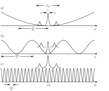
Figure 17: Illustration of the explanation for the different shapes of the emission spectra (see text) for increasing values of $\Gamma_{0}\tau$. The curves in the figures correspond to the function $\sin^{2}(\omega\tau/2)$ for different values of $\tau$. For larger atom-mirror distances the relative variation of this function in a region $\Gamma_{0}$ (the width of the fluorescence triplet) becomes significant and the Markov approximation is not valid anymore. The atom is placed at a node in this example.

Examples obtained from Eq. (78) are shown in Fig. 15 for weak laser intensity and an atom at a node. The spectrum for $\gamma\tau=0$ in this figure is the Mollow result with a damping rate $(1-\varepsilon)\gamma$. The structures arising at large distances resemble those of Fig. 6 and can be interpreted in a similar way. The situation changes in case of higher laser intensities. Examples are shown in Fig. 16a) and 16b) for different values of $\tau$ and different positions of the atom. We see that in general the width of the spectra varies and they are asymmetric depending on the position of the atom.

This behavior can be understood at least on a qualitative level if we take into account that a measure of the coupling strength of the atom to a field mode of frequency $\omega$ is given by $\sin^{2}(\omega\tau/2)$. This function varies in frequency space on a scale $1/\tau$. Defining the quantity $\Gamma_{0}\equiv 2\Omega+\gamma$ which approximately gives the overall width of the triplet we see that for $\Gamma_{0}\tau\ll 1$ (and which we take now as the criterion for small atom-mirror distance) that the coupling is almost flat in the region where the spectrum differs from zero (see Fig. 17a)). This situation corresponds to the Markovian limit discussed in Sec. III.2.1. Thus, we obtain in good approximation the usual Mollow spectrum with a modified spontaneous emission rate $\tilde{\gamma}_{L}$. This is shown in Fig. 16a) for various positions of the atom. The level shift (24b), which acts here as a detuning in case of the dashed line, is so small that this curve cannot be distinguished from the Mollow spectrum with decay rate $\gamma$ on the scale of the figure. For larger values of $\Gamma_{0}\tau$, but still $\gamma\tau\ll 1$ , we have a situation like it is shown in Fig. 17b) where, as an example, an atom located at a node of the standing wave $\sin^{2}(\omega\tau/2)$ is chosen. For increasing laser intensity, the sidebands move towards regions of higher values of the coupling function leading to a higher damping of, say, the corresponding levels in a dressed state picture and thus to a broadening of the sidebands (with increasing laser intensity until $\Omega_{0}\approx\pi/\tau$). For an atom placed at an antinode the behavior is simply the inverse. However, if the atom is placed at a “slope”, e.g. the one on the right hand side of the node which was considered in Fig. 17b), the spectrum becomes asymmetric since the transition responsible for the right sideband is stronger damped than the left one. Thus, the right sideband is broader than the left sideband which is in accordance with the dashed line in Fig. 16b) (For the sake of clarity, the dashed line in this figure is displaced horizontally by a small amount). The case $\Gamma_{0}\tau\gg 1$ is indicated in Fig. 17c) leading to structures as in Fig. 15 or Fig. 6.

So far we have discussed the case of exact resonance ($\Delta=0$) where the emission spectra are symmetric for an atom in a node or an antinode. This situation changes, in general, if we take a finite laser detuning. In case of $\Gamma_{0}\tau\ll 1$ the spectra are approximately identical to the usual Mollow spectra with modified spontaneous emission rate $\tilde{\gamma}_{L}$ and detuning $\tilde{\Delta}$, i.e. they are approximately symmetric independent of the exact atomic position. Examples for this case are shown in Fig. 18a). Note that the sideband positions for an atom located at a slope are shifted towards the central peak which is due to the small frequency shift (the sideband positions are approximately given by $\omega_{L}\pm\sqrt{\Omega_{0}^{2}+(\Delta-\varepsilon\gamma/2\sin(\omega_{L}\tau))^{2}}$).

Figure 18: Incoherent emission spectra for non-vanishing laser detuning ($\Delta=10\gamma$, $\varepsilon=0.2$, $\Omega_{0}=3\gamma$). Fig. a) shows an atom very close to the mirror: The solid line corresponds to node positions ($\omega_{L}\tau=2n\pi$, $\gamma\tau=0.002$), the dashed line to a slope position ($\omega_{L}\tau=(2n+\frac{1}{2})\pi$, $\gamma\tau=0.0025$) and the dotted line to an antinode position ($\omega_{L}\tau=(2n+1)\pi$, $\gamma\tau=0.001$). In Fig. b) $\Gamma_{0}\tau$ is larger. Solid line: $\omega_{L}\tau=2n\pi$, $\gamma\tau=0.15$, dashed line: $\omega_{L}\tau=(2n+\frac{1}{2})\pi$, $\gamma\tau=0.1505$, dotted line: $\omega_{L}\tau=(2n+1)\pi$, $\gamma\tau=0.151$.

This situation differs from that when the distance between the atom and the mirror is increased. Here, the spectra become asymmetric even when the atom is located in a node or an antinode (see Fig. 18b)).

IV Summary

In this work we have discussed the behavior of an atom in the presence of a reflecting wall with regard to pure spontaneous emission, i.e. the decay of an initially excited atom without any laser excitation, and with regard to an additional continuous driving laser field. In the first case, the one dimensional model applied here, can be solved exactly leading to a solution which directly reveals the retarded character of the system (photons bouncing back an forth between the atom and the mirror) visible in the state population, the field intensity and the (transient) photon spectrum. The limit of small distances yields the usual behavior of enhanced and inhibited spontaneous emission which can be interpreted as an interference phenomenon of the the outgoing and reflected light pulse leading to a standing wave pattern in the field intensity: If the atom is placed in an antinode of this standing wave, spontaneous decay is enhanced while in a node it is suppressed. For large distances this interference is not significant anymore and the node-antinode location of the atom becomes less important. The emitted photon wave packet is back reflected by the mirror leading to a partial re-excitation of the atom which starts now to emit again radiation and so on.

In case of an additional driving laser the situation is more complex since the energy of the system increases continuously. Working in a Heisenberg picture we have derived a set of equations which serves as a starting point for several approximative treatments. In the limit of low laser intensities we saw with the help of perturbation theory and a harmonic oscillator model that the system behaves essentially like an atom driven by two monochromatic lasers where the phase difference between the lasers is controlled by the atom-mirror distance. The intensity of the reflected light at the position of the atom depends on the intensity of the driving force on the atom at a preceding time which leads in general to a different state population in every time interval $[m\tau,(m+1)\tau]$ (converging to a steady state value). The dominance of coherent scattering was confirmed by the monochromatic emission spectrum of the system. In this limit we gave also a discussion of the second order intensity correlation function which included in case of the field in channel $1$ an interference of different paths leading to a coincidence signal. This fact causes non-trivial structures in the correlation function.

In case of a higher laser intensity incoherent scattering becomes more significant. However, for small solid angles $\varepsilon$ it is possible to derive a closed set of linear delay differential equations which represents an extension of the usual OBEs. It turned out that an intense laser field can significantly influence the system if we compare it with the Markovian limit where it is possible to describe the system by OBEs with modified decay rate and transition frequency. With regard to the upper state population, for instance, the laser can make the effect of the mirror to disappear regardless of the exact position of the atom (node or antinode). Furthermore, the influence of a strong laser was revealed by the emission spectra. Even if the width of the three peaks of the spectrum are each very small compared to the inverse delay time $\tau$, an intense laser field (or a high detuning) can “push” the sidebands of the triplet towards regions of a higher or lower coupling of the corresponding transitions to the radiation field leading to features like asymmetric spectra (see also mos ).

A possible extension of the discussion presented in this article would be the inclusion of the motional degrees of freedom of the atom. Assuming an atom in a harmonic trap, as in the experimental realization Eschner et al. (2001), the reflected radiation will have an appreciable effect on the center of mass motion of the ion. This can serve as a further probe for effects discussed in this paper. Besides that, collective effects of two ions in the trap, like super- and sub-radiance, could be studied when the image of one ion is projected onto the other. The effect of one atom on another one, mediated by radiation over a large distance, is important for applications like quantum communication S. J. van Enk et al. (1998).

Appendix A The scattered light field

Here we will sketch the derivation of an expression for the field intensity in the channel perpendicular to the mirror which was used for the generation of Fig. 3 and Fig. 5. Besides that, we will give formulae for the electric field operators in the Heisenberg picture which are used in the discussion of laser excitation and an expression for the second order correlation function which is needed to derive Eq. (29). We use the coordinate system introduced in Fig. 1.

The intensity of the emitted light corresponding to Sec. I is defined by

$$I(z,t) = \langle E^{\dagger}(z,t)E(z,t)\rangle=\langle\psi(t)|E^{\dagger}(z)E(z)|\psi(t)\rangle$$ (80)

$$= \left|\text{i}\int\text{d}k\,\alpha_{k}\sin(kz)b_{g,k}^{1}(t)\right|^{2}\equiv|A(z,t)|^{2}.$$

From Eq. (4) we see that

$$A(z,t)= -\varepsilon\frac{\gamma}{2}\frac{\text{i}\hbar}{d}\frac{1}{2\pi}\int_{0}^{t}\text{d}t^{\prime}\,\text{e}^{-\text{i}\omega_{0}t^{\prime}}b_{e}(t^{\prime})$$

$$\times \int\text{d}\omega\,\text{e}^{\text{i}\omega(t^{\prime}-t)}\left(\text{e}^{\text{i}\omega\frac{\tau}{2}}-\text{e}^{-\text{i}\omega\frac{\tau}{2}}\right)\left(\text{e}^{\text{i}\omega\frac{z}{c}}-\text{e}^{-\text{i}\omega\frac{z}{c}}\right),$$ (81)

where the frequency integral gives rise to delta functions which yield non-vanishing terms only in certain regions of space and time,

$$A(z,t)= \varepsilon\frac{\gamma}{2}\frac{\text{i}\hbar}{d}\text{e}^{-\text{i}\omega_{0}t}$$

$$\times\bigg{(} \text{e}^{\text{i}\omega_{0}(\frac{z}{c}-\frac{\tau}{2})}b_{e}(t-{\textstyle\frac{z}{c}}+{\textstyle\frac{\tau}{2}})\Theta(t-{\textstyle\frac{z}{c}}+{\textstyle\frac{\tau}{2}})\Theta({\textstyle\frac{z}{c}}-{\textstyle\frac{\tau}{2}})$$

$$+ \text{e}^{-\text{i}\omega_{0}(\frac{z}{c}-\frac{\tau}{2})}b_{e}(t+{\textstyle\frac{z}{c}}-{\textstyle\frac{\tau}{2}})\Theta(t+{\textstyle\frac{z}{c}}-{\textstyle\frac{\tau}{2}})\Theta({\textstyle\frac{\tau}{2}}-{\textstyle\frac{z}{c}})$$

$$- \text{e}^{\text{i}\omega_{0}(\frac{z}{c}+\frac{\tau}{2})}b_{e}(t-{\textstyle{\textstyle\frac{z}{c}}}-{\textstyle\frac{\tau}{2}})\Theta(t-{\textstyle\frac{z}{c}}-{\textstyle\frac{\tau}{2}})\bigg{)}.$$ (82)

The first and the second line of this expression represent the outgoing light pulses to the right and the left side, respectively while the last line provides us with the reflected light pulse.

In case of laser excitation the appropriate quantity in order to calculate the intensity is the electric field operator in the Heisenberg picture. Starting with the Heisenberg equations (31) and the definitions (2), we use a similar derivation as above, where $A(z,t)$ has to be replaced by the operator $E_{1}(z,t)$ and the amplitude $b_{e}$ by $\sigma_{-}$ (and $\omega_{0}$ by $\omega_{L}$ for a detuned laser). Apart from an additional noise term the result coincides with Eq. (82). On condition that a photo detector is placed on the right hand side of the atom (cf. Fig. 11) at a position $z_{0}>L$ the second line in Eq. (82) does not contribute and one gets

$$E_{1}(d_{0},t)=\varepsilon\frac{\gamma}{2}\frac{\text{i}\hbar}{d} \text{e}^{-\text{i}\omega_{L}(t-\frac{d_{0}}{c})}\bigg{(}\sigma_{-}(t-{\textstyle\frac{d_{0}}{c}})\Theta(t-{\textstyle\frac{d_{0}}{c}})$$

$$-\text{e}^{\text{i}\omega_{L}\tau}\sigma_{-}(t-{\textstyle\frac{d_{0}}{c}}-\tau)\Theta(t-{\textstyle\frac{d_{0}}{c}}-\tau)\bigg{)}$$

$$+N_{1}(d_{0},t)$$ (83)

with

$$N_{1}(d_{0},t)=\frac{\text{i}\hbar}{d}\int\text{d}k\,g_{k}\sin(k(d_{0}+L))a_{k}(0)\text{e}^{-\text{i}\omega_{k}t},$$ (84)

where $d_{0}=z_{0}-L=z_{0}-c\tau/2$ is the distance between the detector and the atom. There are two different kinds of signals arriving at the detector, one which takes its way directly and one which takes the “loop way” over the mirror and therefore needs a longer time.

If the conditions of Sec. III.2.1 are fulfilled, we can approximately calculate the intensity in channel $1$ by neglecting $\tau$ in the arguments of the operators and the step function to obtain

$$\langle E_{1}^{\dagger}(d_{0},t)E_{1}(d_{0},t)\rangle= \left(\frac{\varepsilon\gamma\hbar}{d}\right)^{2}\sin^{2}(\omega_{L}\tau/2)$$

$$\times\langle\sigma_{+}(t-{\textstyle\frac{d_{0}}{c}})\sigma_{-}(t-{\textstyle\frac{d_{0}}{c}})\rangle$$ (85)

which leads to expression (40a) if $d_{0}$ is set to zero.

For the sake of completeness we give here also the electric field in channel 2 since it is used for various calculations,

$$E_{2}(x,t)=\frac{(1-\varepsilon)\gamma}{2}\frac{\text{i}\hbar}{d}\text{e}^{-\text{i}\omega_{L}t}$$

$$\times\bigg{(}\text{e}^{\text{i}\frac{x}{c}}\sigma_{-}(t-{\textstyle\frac{x}{c}})\Theta(t-{\textstyle\frac{x}{c}})\Theta({\textstyle\frac{x}{c}})$$

$$\quad+\text{e}^{-\text{i}\frac{x}{c}}\sigma_{-}(t+{\textstyle\frac{x}{c}})\Theta(t+{\textstyle\frac{x}{c}})\Theta(-{\textstyle\frac{x}{c}})\bigg{)}+N_{2}(x,t)$$ (86)

with

$$N_{2}(x,t)=\frac{\text{i}\hbar}{d}\int\text{d}k\,h_{k}b_{k}(0)\text{e}^{\text{i}(kx-\omega_{k}t)}.$$ (87)

With the help of Eq. (83) one can easily find expressions for the intensity and the first order field correlation function in channel $1$ (the functions connected with the channel $2$ coincide with those of standard Markovian theory).

Using Eq. (83) and the commutation relations (36) we get also an expression for the second order correlation function (25),

$$G^{(2)}_{1}(t,t+T)=\parallel[ \sigma_{-}(t+T)\sigma_{-}(t)$$

$$+ \sigma_{-}(t+T-\tau)\sigma_{-}(t-\tau)$$

$$- \text{e}^{\text{i}\omega_{L}\tau}\sigma_{-}(t+T)\sigma_{-}(t-\tau)$$

$$- \text{e}^{\text{i}\omega_{L}\tau}\mathcal{T}_{{}_{\leftarrow}}\sigma_{-}(t+T-\tau)\sigma_{-}(t)]\,|G\rangle\parallel^{2}.$$ (88)

We set the arbitrary distance $d_{0}$ to zero and omitted the step functions in this expression which is valid if $t>\tau$ (if not, components with negative arguments are simply set to zero). The effect of the non vanishing commutator in Eq. (36) is to conserve time ordering in the last term of Eq. (88), i.e. the time argument of the operator on the left hand side is always greater than the right one. This is indicated by the symbol $\mathcal{T}_{{}_{\leftarrow}}$. We see that for $T<\tau$ and $T>\tau$ the operators have to be exchanged.

Appendix B Some features of the harmonic oscillator model

In order to derive an expression for the correlation functions in the harmonic oscillator model we start with the Heisenberg equation of motion for the operator $c$,

$$\frac{\text{d}}{\text{d}t}c(t)= -\alpha_{1}c(t)+\alpha_{2}c(t-\tau)\Theta(t-\tau)+\alpha_{3}$$

$$+\frac{\text{i}d}{\hbar}\text{e}^{\text{i}\omega_{L}t}\big{(}N_{1}(t)+N_{2}(t)\big{)}.$$ (89)

with parameters $\alpha_{i}$ are defined in Sec. III.2.2 and noise operators given by (34). Let us define a vector

$$|\Psi(t)\rangle\equiv c(t)|\psi(0)\rangle,\quad\text{i.e.}\quad|\Psi(0)\rangle=c(0)|\psi(0)\rangle,$$ (90)

where $|\psi(0)\rangle\equiv|\varphi,\{0\}_{1},\{0\}_{2}\rangle$ is the initial state of the system. The state

$$|\varphi\rangle=a|g\rangle+b|e\rangle,\quad|a|^{2}+|b|^{2}=1$$ (91)

is an arbitrary state on the atomic space. Eq. (89) provides us with an equation of motion for this vector,

$$\frac{\text{d}}{\text{d}t}|\Psi(t)\rangle= -\alpha_{1}|\Psi(t)\rangle+\alpha_{2}|\Psi(t-\tau)\rangle\Theta(t-\tau)$$

$$+\alpha_{3}|\psi(0)\rangle.$$ (92)

Thus we have a linear inhomogeneous delay differential equation and its solution takes the form

$$|\Psi(t)\rangle=\text{A}(t)|\psi(0)\rangle+\text{B}(t)|\Psi(0)\rangle.$$ (93)

This vector has the form $|\chi(t)\rangle|\{0\}_{1},\{0\}_{2}\rangle$ where the non-constant part is an element of the atomic Hilbert space. The coefficients are given by

$$\text{A}(t) =\frac{\alpha_{3}}{\alpha_{1}}\sum_{n=0}^{\infty}\frac{\alpha_{2}^{n}}{n!}(t-n\tau)^{n}G_{n}[-\alpha_{1}(t-n\tau)]\Theta(t-\tau),$$ (94)

$$\text{B}(t) =\sum_{n=0}^{\infty}\frac{\alpha_{2}^{n}}{n!}(t-n\tau)^{n}\text{e}^{-\alpha_{1}(t-n\tau)}\Theta(t-n\tau).$$ (95)

These expressions can be found by Laplace transformation in a way it was demonstrated in Eq. (LABEL:eq:demo) (the function $G_{n}$ is defined in Eq. (14)).

Some expectation values of interest are

$$\langle c(t)\rangle=\langle\psi(0)|\Psi(t)\rangle=\text{A}(t)+\text{B}(t)\langle c(0)\rangle,$$ (96)

$$\langle c^{\dagger}(t)c(t)\rangle=\||\Psi(t)\rangle\|^{2}$$

$$\quad=\langle c^{\dagger}(t)\rangle\langle c(t)\rangle+|\text{B}(t)|^{2}\big{(}\langle c^{\dagger}(0)c(0)\rangle-\langle c^{\dagger}(0)\rangle\langle c(0)\rangle\big{)}.$$ (97)

From the above expressions it is immediately clear that

$$\langle c^{\dagger}(t)c(t)\rangle=\langle c^{\dagger}(t)\rangle\langle c(t)\rangle\quad\forall\,t>0$$ (98)

if $\langle c^{\dagger}(0)c(0)\rangle=\langle c^{\dagger}(0)\rangle\langle c(0)\rangle$, which is the case iff the atom is initially in the ground state. In the long time limit this behavior is independent of the initial state, i.e. $\langle c^{\dagger}c\rangle_{ss}=\langle c^{\dagger}\rangle_{ss}\langle c\rangle_{ss}$ since $\underset{t\rightarrow\infty}{\lim}\text{B}(t)=0$.

If we start in the ground state the harmonic oscillator model reproduces result (22) gained from the perturbation theory and a remarkable fact is that Eq. (97) also reproduces the solution (7) obtained from the modified Wigner-Weisskopf theory if we set $\alpha_{3}=0$ (no laser) so that $\text{A}(t)=0$ for all $t$ and $|\varphi\rangle=|e\rangle$.

The two-time correlation functions take the form

$$\langle c^{\dagger}(t^{\prime})c(t)\rangle=\langle\Psi(t^{\prime})|\Psi(t)\rangle$$

$$\quad=\langle c^{\dagger}(t^{\prime})\rangle\langle c(t)\rangle+\text{B}^{*}(t^{\prime})\text{B}(t)\big{(}\langle c^{\dagger}c(0)\rangle-\langle c^{\dagger}(0)\rangle\langle c(0)\rangle\big{)},$$ (99)

where the time order is irrelevant. We see again that this quantity factorizes in special cases,

$$\langle c^{\dagger}(t^{\prime})c(t)\rangle=\langle c^{\dagger}(t^{\prime})\rangle\langle c(t)\rangle,\quad\text{if}\,|\varphi\rangle=|g\rangle,$$

$$\underset{t\rightarrow\infty}{\lim}\langle c^{\dagger}(t+T)c(t)\rangle=\langle c^{\dagger}\rangle_{ss}\langle c\rangle_{ss},\quad\forall\,|\varphi\rangle.$$ (100)

In order to derive fourth order correlation functions we proceed in a similar way. We define a vector

$$|\Phi(t^{\prime})\rangle \equiv c(t^{\prime})|\Psi(t)\rangle,$$ (101)

$$|\Phi(0)\rangle = c(0)|\Psi(t)\rangle=\text{A}(t)|\Psi(0)\rangle.$$ (102)

For this vector we get again an equation of the form (92) where we replace $|\Psi(t)\rangle\rightarrow|\Phi(t^{\prime})\rangle$ and $|\psi(0)\rangle\rightarrow|\Psi(t)\rangle$ which finally gives the fourth order correlation function

$$G^{(2)}_{2}(t,t+T) = \langle c^{\dagger}(t)c^{\dagger}(t+T)c(t+T)c(t)\rangle$$ (103)

$$= \||\Phi(t+T)\rangle\|^{2}$$

which leads to

$$G^{(2)}_{2}(t,t+T)=\|\big{(} A(t)A(t+T)+A(t+T)B(t)c(0)$$

$$+ A(t)B(t+T)c(0)\big{)}|\psi(0)\rangle\|^{2},$$ (104)

and thus,

$$G^{(2)}_{2}(t,t+T)=\langle c^{\dagger}(t)c(t)\rangle\langle c^{\dagger}(t+T)c(t+T)\rangle,\,|\varphi\rangle=|g\rangle,$$

$$\underset{t\rightarrow\infty}{\lim}G^{(2)}_{2}(t,t+T)=\langle c^{\dagger}c\rangle_{ss}^{2},\quad\forall\,|\varphi\rangle.$$ (105)

From Eq. (88) we also obtain

$$\underset{t\rightarrow\infty}{\lim}G^{(2)}_{1}(t,t+T)=16\sin^{4}(\omega_{L}\tau/2)\langle c^{\dagger}c\rangle_{ss}^{2},\quad\forall\,|\varphi\rangle.$$ (106)

This result is equal to the square of the intensity in the long time limit in this channel.

Appendix C Calculation of the spectrum

In this appendix a sketch of the derivation of the emission spectrum in case of a higher laser intensity is outlined. We will indicate in the following merely retarded time arguments. In order to get Eq. (77) and Eq. (78) we consider the operators

$$\delta A \equiv \delta\sigma_{-}\delta b_{\omega}=\sigma_{-}b_{\omega}+\langle\sigma_{-}\rangle\langle b_{\omega}\rangle-b_{\omega}\langle\sigma_{-}\rangle-\sigma_{-}\langle b_{\omega}\rangle,$$

$$\delta B \equiv \delta\sigma_{+}\delta b_{\omega}=\sigma_{+}b_{\omega}+\langle\sigma_{+}\rangle\langle b_{\omega}\rangle-b_{\omega}\langle\sigma_{+}\rangle-\sigma_{+}\langle b_{\omega}\rangle,$$

$$\delta C \equiv \delta\sigma_{z}\delta b_{\omega}=\sigma_{z}b_{\omega}+\langle\sigma_{z}\rangle\langle b_{\omega}\rangle-b_{\omega}\langle\sigma_{z}\rangle-\sigma_{z}\langle b_{\omega}\rangle.$$

After transforming in a rotating frame, $\delta A\rightarrow\text{e}^{-2\text{i}\omega_{L}t}\delta A$, $\delta B\rightarrow\delta B$, $\delta C\rightarrow\text{e}^{-\text{i}\omega_{L}t}\delta C$, $\sigma_{-}\rightarrow\text{e}^{-\text{i}\omega_{L}t}\sigma_{-}$, $b_{\omega}\rightarrow\text{e}^{-\text{i}\omega t}b_{\omega}$, the Heisenberg equations of motion for these operators yield, after taking the expectation value, Eq. (77),

$$\dot{\vec{P}}(t)=\big{[}-\text{i}(\omega-\omega_{0})\openone+A_{3}\big{]}\vec{P}(t)+\kappa_{\omega}\vec{I}_{0}(t)+\varepsilon\vec{I}(t,\tau),$$ (108)

where $\vec{P}(t)$ is defined in Eq. (76) and

$$A_{3} \equiv \begin{pmatrix}-\frac{\gamma}{2}-\text{i}\Delta&0&-\text{i}\frac{\Omega_{0}}{2}\\ 0&-\frac{\gamma}{2}+\text{i}\Delta&\text{i}\frac{\Omega_{0}}{2}\\ -\text{i}\Omega_{0}&\text{i}\Omega_{0}&-\gamma\end{pmatrix},$$ (109)

$$\vec{I}_{0}(t) = \begin{pmatrix}-\langle\sigma_{-}\rangle^{2}\\ \langle\sigma_{+}\sigma_{-}\rangle-\langle\sigma_{+}\rangle\langle\sigma_{-}\rangle\\ -2\langle\sigma_{+}\sigma_{-}\rangle\langle\sigma_{-}\rangle\end{pmatrix}.$$ (110)

The components of $I(t,\tau)$ are given by

$$I_{1}(t,\tau)= -\frac{\gamma}{2}\text{e}^{\text{i}\omega_{L}\tau}\big{(}\langle\delta C\sigma_{-}(t-\tau)\rangle+\langle\sigma_{z}\rangle h_{-}(t,\tau)\big{)}$$

$$I_{2}(t,\tau)= -\frac{\gamma}{2}\text{e}^{-\text{i}\omega_{L}\tau}\big{(}\langle\sigma_{+}(t-\tau)\delta C\rangle+\langle\sigma_{z}\rangle h_{+}(t,\tau)\big{)}$$

$$I_{3}(t,\tau)= \quad\gamma\text{e}^{-\text{i}\omega_{L}\tau}\big{(}\langle\sigma_{+}(t-\tau)\delta A\rangle+\langle\sigma_{-}\rangle h_{+}(t,\tau)\big{)}$$

$$+\gamma\text{e}^{\text{i}\omega_{L}\tau}\big{(}\langle\delta B\sigma_{-}(t-\tau)\rangle+\langle\sigma_{+}\rangle h_{-}(t,\tau)\big{)}$$ (111)

with

$$h_{-}(t,\tau)\equiv\langle\delta b_{\omega}\sigma_{-}(t-\tau)\rangle\text{e}^{\text{i}(\omega_{L}-\omega)t},$$ (112)

$$h_{+}(t,\tau)\equiv\langle\sigma_{+}(t-\tau)\delta b_{\omega}\rangle\text{e}^{\text{i}(\omega_{L}-\omega)t},$$ (113)

where only retarded time arguments are indicated. The quantities $h_{\pm}$ can be calculated with the help of the Heisenberg equations of motion for $b_{\omega}$. The result contains atomic two time correlation functions which have to be calculated again in $0$-th order $\varepsilon$ depending on the initial state which is a single time expectation value. The calculation of the correlation functions contained in (111) is analogous to the calculation done to derive the delay OBEs (60): We multiply the Heisenberg equations of motion for the operators (LABEL:eq:delta_operators) once from the left with $\sigma_{+}(t^{\prime})$ and once from the right with $\sigma_{-}(t^{\prime})$ ($t^{\prime}\leq t$) and keep only terms of first order in $\varepsilon$. The six equations we get in this way now contain again atomic two time correlation functions which have to be calculated as it was done for $h_{\pm}$. Then we let $t\rightarrow\infty$ and get an expression of the form (78) with

$$\tilde{K}(\tau)=\begin{pmatrix}\frac{\gamma}{2}\tilde{f}_{1}(\tau)&0&-\text{i}\frac{\Omega_{0}}{2}\tilde{f}_{2}(\tau)\\ 0&\frac{\gamma}{2}\tilde{f}_{1}^{*}(\tau)&\text{i}\frac{\Omega_{0}}{2}\tilde{f}_{2}^{*}(\tau)\\ -\text{i}\Omega_{0}\tilde{f}_{3}(\tau)&\text{i}\Omega_{0}\tilde{f}_{3}^{*}(\tau)&\gamma\tilde{f}_{4}(\tau)\end{pmatrix},$$ (114)

$$\tilde{f}_{1}(\tau)=-\text{e}^{\text{i}\omega_{L}\tau}g_{z}(\tau),$$ (115)

$$\tilde{f}_{2}(\tau)=-\frac{\text{i}\gamma}{2\Omega_{0}}\text{e}^{\text{i}\omega_{L}\tau}U_{31}^{*}(\tau),$$ (116)

$$\tilde{f}_{3}(\tau)=\frac{\text{i}\gamma}{\Omega_{0}}\text{e}^{\text{i}\omega_{L}\tau}g_{+}(\tau),$$ (117)

$$\tilde{f}_{4}(\tau)=\frac{1}{2}\big{(}\text{e}^{-\text{i}\omega_{L}\tau}U_{11}(\tau)+\text{e}^{\text{i}\omega_{L}\tau}U_{11}^{*}(\tau)\big{)},$$ (118)

and

$$\begin{pmatrix}g_{-}(\tau)\\ g_{+}(\tau)\\ g_{z}(\tau)\end{pmatrix}=U(\tau)\left[\begin{pmatrix}0\\ 0\\ -1\end{pmatrix}-\begin{pmatrix}\langle\sigma_{-}\rangle_{ss}\\ \langle\sigma_{+}\rangle_{ss}\\ \langle\sigma_{z}\rangle_{ss}\end{pmatrix}\right]+\begin{pmatrix}\langle\sigma_{-}\rangle_{ss}\\ \langle\sigma_{+}\rangle_{ss}\\ \langle\sigma_{z}\rangle_{ss}\end{pmatrix}.$$ (119)

The inhomogeneity $I_{1}(\tau)$ in Eq. (78) is so lengthy that we do not quote it here.

References

• Berman (1994) P. R. Berman, ed., Cavity Quantum Electrodynamcis, Advances in Atomic, Molecular, and Optical Physics, Suppl. 2 (Academic Press, Boston, 1994).
• Hinds (1991) E. A. Hinds, in Advances in Atomic, Molecular, and Optical Physics, edited by D. Bates and B. Bederson (Academic Press, Boston, 1991), vol. 28, p. 237.
• Haroche (1990) S. Haroche, in Fundamental Systems in Quantum Optics, edited by J. Dalibard, J.-M. Raimond, and J. Zinn-Justin (North-Holland, Amsterdam, 1990), Les Houches Session LIII, p. 767.
• Heinzen et al. (1987) D. J. Heinzen, J. J. Childs, J. E. Thomas, and M. S. Feld, Phys. Rev. Lett. 58, 1320 (1987).
• Heinzen and Feld (1987) D. J. Heinzen and M. S. Feld, Phys. Rev. Lett. 59, 2623 (1987).
• Jhe et al. (1987) W. Jhe, A. Anderson, E. A. Hinds, D. Meschede, L. Moi, and S. Haroche, Phys. Rev. Lett. 58, 666 (1987).
• Hulet et al. (1985) R. G. Hulet, E. S. Hilfer, and D. Kleppner, Phys. Rev. Lett. 55, 2137 (1985).
• Goy et al. (1983) P. Goy, J. M. Raimond, M. Gross, and S. Haroche, Phys. Rev. Lett. 50, 1903 (1983).
• DeMartini et al. (1987) F. DeMartini, G. Innocenti, G. R. Jacobovitz, and P. Mataloni, Phys. Rev. Lett. 59, 2955 (1987).
• (10) See E. A. Hinds in Berman (1994).
• Hood et al. (2000) C. J. Hood, T. W. Lynn, A. C. Doherty, A. S. Parkins, and H. J. Kimble, Science 287, 1447 (2000).
• Pinkse et al. (2000) P. W. H. Pinkse, T. Fischer, P. Maunz, and G. Rempe, Nature 404, 365 (2000).
• (13) A. B. Mundt, A. Kreuter, C. Becher, D. Leibfried, J. Eschner, F. Schmidt-Kaler, and R. Blatt, eprint quant-ph/0202112.
• Guthöhrlein et al. (2001) G. R. Guthöhrlein, M. Keller, K. Hayasaka, W. Lange, and H. Walther, Nature 414, 49 (2001).
• Raimond et al. (2001) J. M. Raimond, M. Brune, and S. Haroche, Rev. Mod. Phys. 73, 565 (2001).
• (16) See G. Raithel and C. Wagner and H. Walther and L. M. Narducci and M. O. Scully in Berman (1994).
• Eschner et al. (2001) J. Eschner, C. Raab, F. Schmidt-Kaler, and R. Blatt, Nature 413, 495 (2001).
• Milonni (1994) P. W. Milonni, The Quantum Vacuum (Academic Press, Boston, 1994).
• Meschede et al. (1990) D. Meschede, W. Jhe, and E. A. Hinds, Phys. Rev. A 41, 1587 (1990).
• Hinds and Sandoghdar (1991) E. A. Hinds and V. Sandoghdar, Phys. Rev. A 43, 398 (1991).
• Milonni et al. (1983) P. W. Milonni, J. R. Ackerhalt, H. W. Galbraith, and Mei-Li Shih, Phys. Rev. A 28, 32 (1983).
• Cook and Milonni (1987) R. J. Cook and P. W. Milonni, Phys. Rev. A 35, 5081 (1987).
• Feng and Ujihara (1990) X.-P. Feng and K. Ujihara, Phys. Rev. A 41, 2668 (1990).
• Dung and Ujihara (1999) H. T. Dung and K. Ujihara, Phys. Rev. A 60, 4067 (1999).
• Milonni and Knight (1974) P. W. Milonni and P. L. Knight, Phys. Rev. A 10, 1096 (1974).
• Milonni and Knight (1975) P. W. Milonni and P. L. Knight, Phys. Rev. A 11, 1090 (1975).
• Parker and C. R. Stroud Jr. (1987) J. Parker and C. R. Stroud Jr., Phys. Rev. A 35, 4226 (1987).
• Gießen et al. (1996) H. Gießen, J. D. Berger, G. Mohs, P. Meystre, and S. F. Yelin, Phys. Rev. A 53, 2816 (1996).
• Bužek et al. (1999) V. Bužek, G. Drobný, M. G. Kim, M. Havukainen, and P. L. Knight, Phys. Rev. A 60, 582 (1999).
• Wiseman (1994) H. M. Wiseman, Phys. Rev. A 49, 2133 (1994).
• Wiseman and Milburn (1994) H. M. Wiseman and G. J. Milburn, Phys. Rev. A 49, 4110 (1994).
• Giovannetti et al. (1999) V. Giovannetti, P. Tombesi, and D. Vitali, Phys. Rev. A 60, 1549 (1999).
• Wang et al. (2001) J. Wang, H. M. Wiseman, and G. J. Milburn, Chem. Phys. 268, 221 (2001).
• Driver (1977) R. D. Driver, Ordinary and Delay Differential Equations, vol. 20 of Applied Mathematical Sciences (Springer, New York, 1977).
• Carmichael (1993) H. J. Carmichael, Phys. Rev. Lett. 70, 2273 (1993).
• Gardiner (1993) C. W. Gardiner, Phys. Rev. Lett. 70, 2269 (1993).
• Kochan and Carmichael (1994) P. Kochan and H. J. Carmichael, Phys. Rev. A 50, 1700 (1994).
• Gardiner and Parkins (1994) C. W. Gardiner and A. S. Parkins, Phys. Rev. A 50, 1792 (1994).
• Gardiner and Zoller (2000) C. W. Gardiner and P. Zoller, Quantum Noise (Springer, Berlin, 2000), 2nd ed.
• Glauber (1963) R. J. Glauber, Phys. Rev. 130, 2529 (1963).
• Allen and Eberly (1987) L. Allen and J. H. Eberly, Optical Resonance and Two-Level Atoms (Dover Publications, New York, 1987).
• Erdélyi et al. (1954) A. Erdélyi, W. Magnus, F. Oberhettinger, and F. G. Tricomi, Tables of Integral Transforms, vol. I (McGraw-Hill, New York, 1954).
• Knight and Milonni (1980) P. L. Knight and P. W. Milonni, Phys. Rep. 66, 21 (1980).
• Mollow (1969) B. R. Mollow, Phys. Rev. 188, 1969 (1969).
• (45) See T. W. Mossberg and M. Lewenstein in Berman (1994).
• S. J. van Enk et al. (1998) S. J. van Enk, J. I. Cirac, and P. Zoller, Science 279, 205 (1998).