Purification and detection of entangled coherent states

Abstract

In [J. C. Howell and J. A. Yeazell, Phys. Rev. A 62, 012102 (2000)], a proposal is made to generate entangled macroscopically distinguishable states of two spatially separated traveling optical modes. We model the decoherence due to light scattering during the propagation along an optical transmission line and propose a setup allowing an entanglement purification from a number of preparations which are partially decohered due to transmission. A purification is achieved even without any manual intervention. We consider a nondemolition configuration to measure the purity of the state as contrast of interference fringes in a double-slit setup. Regarding the entangled coherent states as a state of a bipartite quantum system, a close relationship between purity and entanglement of formation can be obtained. In this way, the contrast of interference fringes provides a direct means to measure entanglement.

I Introduction

The preparation of two spatially separated traveling optical modes in entangled coherent states is of special interest since by representing an outcome of Schrödinger’s thought experiment Schrödinger (1935) and at the same time a state of a bipartite quantum system Bennett et al. (1996), it provides a link between philosopical underpinnings of quantum mechanics and applications in quantum information processing. On the other hand, this state has a chance of its experimental realization in the laboratory.

In this paper, we continue the study of two-mode entangled coherent states, whose preparation is investigated in Howell and Yeazell (2000a). The setup considered in Howell and Yeazell (2000a) applies a Mach-Zehnder interferometer equipped with a cross-Kerr element in each of two spatially separated modes. In turn, it may be regarded as a two-mode extension of an analogous single-mode configuration that is proposed in Gerry (1999) to prepare a superposition of two single-mode coherent states. Here, we put emphasis on the state transmission, purification and detection as subsequent steps of quantum state engineering. In doing so, these schemes can be linked to other work on detection and application of single- and two-mode quantum states. For example, a double-slit configuration in combination with a cross-Kerr element is used in Filip to measure in terms of interference fringe contrast a variety of quantities representing measures of quantum state distance. Moreover, there is a number of works treating the properties of general interferometry with entangled coherent states Rice and Sanders (1998); Sanders and Rice (1999, 2000); Rice et al. (2000); Bartlett et al. (2001). Applications to quantum teleportation of one qubit are considered in Lee and Kim (2000) for the example of entangled single-photon states and in van Enk and Hirota (2001) for the example of entangled coherent states. In Lee and Kim (2000) also Bell’s inequality is studied and in van Enk and Hirota (2001) the effect of decoherence is analysed. A quantum nondemolition setup to detect presence of a single photon is proposed in Howell and Yeazell (2000b).

In the present work, we pay special attention to entanglement purification, which plays an important role in quantum information processing Bennett et al. (1996) and becomes a delicate issue especially if entangled macroscopically distinguishable quantum states are involved. In particular, we address the question of state evolution if a setup implementing an entanglement purification protocol is left on its own. It turns out that the state purifies itself, albeit with random parity.

The state preparation is achieved by a conditional state reduction connected with a measurement. With the consideration of a spatially extented configuration, the concept of entanglement comes into play. Entanglement cannot be observed in a local context. Therefore, for a such a conditional scheme to be meaningful, there should be an observer who, like a viewer of the drawings in the figures below, has an overlook of the actions performed elsewhere and their results. In our setups, this will be a third party located halfway between the two entangled parties and which communicates with them either by a classical or a quantum channel. Below, we will see that either channel type may be used, depending on the experimental situation.

II State preparation and transmission

The scheme relies on cross-Kerr couplers described by operators $\hat{K}_{jk}$ $\!=$ $\!\mathrm{e}^{\mathrm{i}\pi\hat{n}_{j}\hat{n}_{k}}$, where $\hat{n}_{j}$ $\!=$ $\hat{a}_{j}^{\dagger}\hat{a}_{j}$, and beam splitters described by operators $\hat{U}_{jk}(T,R)$ defined via the relation

$$\hat{U}_{jk}^{\dagger}\binom{\hat{a}_{j}}{\hat{a}_{k}}\hat{U}_{jk}=\left(\begin{array}[]{cc}T&R\\ -R^{*}&T^{*}\end{array}\right)\binom{\hat{a}_{j}}{\hat{a}_{k}}$$ (1)

by their complex transmittance $T$ and reflectance $R$ obeying $|T|^{2}$ $\!+$ $\!|R|^{2}$ $\!=$ $\!1$. We start with the state preparation. Fig. 1 shows the overall setup.

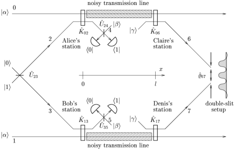
Figure 1: Preparation, transmission and detection of entangled mesoscopic coherent states. The entanglement remaining after having been subjected to scattering loss during transmission is measured as the contrast of interference fringes seen in a double-slit setup.

The source of the entangled state consists of a device able to prepare a pulse in a single-photon state $|1\rangle$, which is fed into one of the input ports of a balanced beam splitter $\hat{U}_{23}(T=-R=1/\sqrt{2})$ whose second input port remains in the vacuum state $|0\rangle$. The pulse leaving this beam splitter is therefore prepared in an entangled two-mode state

$$\hat{U}_{23}|1\rangle_{2}|0\rangle_{3}=\frac{|0\rangle_{2}|1\rangle_{3}+|1\rangle_{2}|0\rangle_{3}}{\sqrt{2}},$$ (2)

with a mode 2 traveling to Alice’s and a mode 3 traveling to Bob’s station. Alice and Bob use cross-Kerr couplers $\hat{K}_{02}$ and $\hat{K}_{13}$ to mix the received pulse with an incoming signal pulse corresponding to their signal mode 0 and 1, respectively. After that, each of them mixes the pulse from $\hat{U}_{23}$ with one prepared in a coherent state $|\beta\rangle$ $\!=$ $\!\exp(-|\beta|^{2}/2)\sum_{k}\beta^{k}/\sqrt{k!}|k\rangle$ (mode 4 and 5) using identical beam splitters $\hat{U}_{24}(T,R)$ and $\hat{U}_{35}(T,R)$, respectively, and performs photon number measurements.

If Alice and Bob detect with their photodetectors 0 and 1 photons as depicted in Fig. 1, their combined action on the signal state can be described by a (“conditional” ) two-mode operator

$$\hat{Y} = \,{}_{2}\langle 1|\,_{3}\langle 1|\,_{4}\langle 0|\,_{5}\langle 0|\hat{U}_{35}\hat{U}_{24}\hat{K}_{13}\hat{K}_{02}|\beta\rangle_{4}|\beta\rangle_{5}\hat{U}_{23}|1\rangle_{2}|0\rangle_{3}$$ (3)

$$= \frac{TR\langle 0|\beta\rangle\langle 1|\beta\rangle}{\sqrt{2}}[(-1)^{\hat{n}_{0}}+(-1)^{\hat{n}_{1}}].$$

Note that with regard to the detection result as shown in Fig. 1, Alice’s photodetectors together with the beam splitter $\hat{U}_{24}$ and the coherent state input may be regarded as a unit performing a detection

$$\,{}_{2}\langle 1|\,_{4}\langle 0|\hat{U}_{24}|\beta\rangle_{4}=\mathrm{e}^{-\frac{|\beta|^{2}}{2}}\Bigl{(}\,_{2}\langle 1|\,T+\,_{2}\langle 0|\,R\beta\Bigr{)}$$ (4)

in mode 2 (the same holds for the corresponding unit on Bob’s side). When Alice’s and Bob’s signal pulses are initially prepared in coherent states $|\alpha\rangle$, the two-mode state of the signal pulses leaving $\hat{K}_{02}$ and $\hat{K}_{13}$ becomes

$$|\Psi\rangle_{01} = \frac{1}{\sqrt{p}}\hat{Y}|\alpha\rangle_{0}|\alpha\rangle_{1}$$ (5)

$$= \frac{|\alpha\rangle_{0}|\!-\!\alpha\rangle_{1}+|\!-\!\alpha\rangle_{0}|\alpha\rangle_{1}}{\sqrt{2(1+\mathrm{e}^{-4|\alpha|^{2}})}}.$$

The probability

$$p = \,{}_{0}\langle\alpha|\,_{1}\langle\alpha|\hat{Y}^{\dagger}\hat{Y}|\alpha\rangle_{0}|\alpha\rangle_{1}$$ (6)

$$= |TR\langle 0|\beta\rangle\langle 1|\beta\rangle|^{2}(1+\mathrm{e}^{-4|\alpha|^{2}})$$

takes for $|T|^{2}$ $\!=$ $\!|\beta|^{2}$ $\!=$ $\!1/2$ the maximal value

$$p_{\mathrm{max}}=\frac{1+\mathrm{e}^{-4|\alpha|^{2}}}{8\mathrm{e}}\approx(8\mathrm{e})^{-1}\approx 5\%,$$ (7)

which becomes for sufficiently large $|\alpha|$ independent of $\alpha$. Finally, the classical trigger signal confirming the desired photodetection result is sent to an (observing) third party.

We see that Eq. (5) is a superposition of macroscopically distinguishable states $|\alpha\rangle_{0}|\!-\!\alpha\rangle_{1}$ and $|\!-\!\alpha\rangle_{0}|\alpha\rangle_{1}$. This means that the two-mode entanglement of a single photon triggers the preparation of entangled coherent states with arbitrarily large amplitude $|\alpha|$. With regard to entanglement, the case $|\alpha|$ $\!\gg$ $\!1$ describes the situation of two Schrödinger’s cats Schrödinger (1935): The entangled single-photon state Eq. (2) represents the (microscopic) radioactive atom, the devices at Alice’s and Bob’s station represent the (amplifying) mechanisms releasing the poison, and the signal pulse whose state changes from the initial product state $|\alpha\rangle_{0}|\alpha\rangle_{1}$ to Eq. (5) represents two (macroscopic) cats, one of which is killed but it is uncertain which one.

• Alternative:

The state Eq. (5) can also be generated if Alice and Bob prepare the second input modes of $\hat{K}_{02}$ and $\hat{K}_{13}$ in coherent states $|\beta\rangle$ and send the respective output pulses to a third location where they are mixed using a beam splitter $\hat{U}_{23}^{\dagger}$. If behind this beam splitter 1 and 0 photons are detected in mode 2 and 3, respectively, their action can again be described by a conditional operator

$$\hat{\tilde{Y}} = \,{}_{2}\langle 1|\,_{3}\langle 0|\hat{U}_{23}^{\dagger}\hat{K}_{13}\hat{K}_{02}|\beta\rangle_{2}|\beta\rangle_{3}$$ (8)

$$= \frac{\langle 0|\beta\rangle\langle 1|\beta\rangle}{\sqrt{2}}[(-1)^{\hat{n}_{0}}+(-1)^{\hat{n}_{1}}],$$

and the signal state reads

$$\frac{1}{\sqrt{\tilde{p}}}\hat{\tilde{Y}}|\alpha\rangle_{0}|\alpha\rangle_{1}=|\Psi\rangle_{01}.$$ (9)

For $\beta$ $\!=$ $\!1/\sqrt{2}$ the success probability becomes $\tilde{p}$ $\!=$ $\!4p_{\mathrm{max}}$, compare Eq. (5) and Eq. (7). The result of this measurement does of course not affect the reduced signal state

$$\mathrm{Tr}_{2}\Bigl{(}\hat{K}_{02}|\alpha\rangle_{0}|\beta\rangle_{2}\,{}_{0}\langle\alpha|\,_{2}\langle\beta|\hat{K}_{02}^{\dagger}\Bigr{)}$$

$$=C(|\beta|^{2})|\alpha\rangle_{0}\langle\alpha|+S(|\beta|^{2})|\!-\!\alpha\rangle_{0}\langle-\alpha|$$ (10)

as observed by Alice (analogously Bob) locally. It only changes the information available at the third location. In Eq. (10) we have used the functions

$$C(x) = \mathrm{e}^{-x}\cosh x,$$ (11a)

$$S(x) = \mathrm{e}^{-x}\sinh x.$$ (11b)

Let us now consider the transmission of a signal in a two-mode state $\hat{\varrho}(x)$ along a lossy transmission line ranging from $x$ $\!=$ $\!0$ to $x$ $\!=$ $\!l$ (cf. Fig. 1). In order to model the scattering loss occuring during transmission, we insert at locations $x_{k}$ $\!=$ $\!kL/n$, $k$ $\!=$ $\!0,1,\ldots$ beam splitters $\hat{U}_{0k}$ with transmittances $\!T_{0}^{1/n}$ in Alice’s signal mode and beam splitters $\hat{U}_{1k}$ with transmittances $\!T_{1}^{1/n}$ in Bob’s signal mode Schubert and Weber (1993). Here, $T_{0/1}$ $\!\in$ $\![0,1]$ define the scattering losses per given length $L$. If all the second input modes of these beam splitters are in the vacuum state, we obtain the relation

$$\hat{\varrho}(x+L/n) = \mathrm{Tr}_{kk^{\prime}}\left[\hat{U}_{1k^{\prime}}\hat{U}_{0k}|0\rangle_{kk^{\prime}}\hat{\varrho}(x)\,_{kk^{\prime}}\langle 0|\hat{U}_{0k}^{\dagger}\hat{U}_{1k^{\prime}}^{\dagger}\right]$$ (12)

$$= \sum_{l,l^{\prime}=0}^{\infty}\frac{(T_{0}^{-2/n}-1)^{l}(T_{1}^{-2/n}-1)^{l^{\prime}}}{l!l^{\prime}!}$$

$$\times\hat{a}_{1}^{l^{\prime}}\hat{a}_{0}^{l}T_{1}^{\frac{\hat{n}_{1}}{n}}T_{0}^{\frac{\hat{n}_{0}}{n}}\hat{\varrho}(x)T_{0}^{\frac{\hat{n}_{0}}{n}}T_{1}^{\frac{\hat{n}_{1}}{n}}\hat{a}_{0}^{\dagger\,l}\hat{a}_{1}^{\dagger\,l^{\prime}}.$$

By expanding the exponentials and replacing differences with differentials one may verify that in the limit $n$ $\!\rightarrow$ $\!\infty$, Eq. (12) yields the well-known master equation of two damped harmonic oscillators Walls and Milburn (1994)

$$L\frac{\mathrm{d}\hat{\varrho}(x)}{\mathrm{d}x}=\ln T_{0}\mathcal{L}_{0}\hat{\varrho}(x)+\ln T_{1}\mathcal{L}_{1}\hat{\varrho}(x),$$ (13)

where

$$\mathcal{L}_{j}\hat{\varrho}=\hat{n}_{j}\hat{\varrho}-2\hat{a}_{j}\hat{\varrho}\hat{a}_{j}^{\dagger}+\hat{\varrho}\hat{n}_{j}.$$ (14)

(Note that the unitary state evolution describing the pulse propagation in free space is taken into account in the interaction picture, which may be envisaged as changing to a co-rotating frame in phase space.) It is sufficient to limit attention to states of the form

$$\hat{\varrho}(x)=\frac{\hat{\rho}_{\mathrm{inc}}+r\hat{\rho}_{\mathrm{coh}}}{2[1+r\mathrm{e}^{-2(|\alpha_{0}|^{2}+|\alpha_{1}|^{2})}]},$$ (15)

where

$$\hat{\rho}_{\mathrm{inc}} = |\alpha_{0},-\alpha_{1}\rangle\langle\alpha_{0},-\alpha_{1}|+|\!-\!\alpha_{0},\alpha_{1}\rangle\langle-\alpha_{0},\alpha_{1}|,$$

$$\hat{\rho}_{\mathrm{coh}} = |\alpha_{0},-\alpha_{1}\rangle\langle-\alpha_{0},\alpha_{1}|+|\!-\!\alpha_{0},\alpha_{1}\rangle\langle\alpha_{0},-\alpha_{1}|$$

($|\alpha,\beta\rangle$ $\!\equiv$ $\!|\alpha\rangle_{0}|\beta\rangle_{1}$), with $\alpha_{j}$ $\!=$ $\!\alpha_{j}(x)$ being the complex amplitude and $r$ $\!=$ $\!r(x)$ being the purity parameter. To see this, consider Alice’s and Bob’s signal pulses which, after leaving $\hat{K}_{02}$ and $\hat{K}_{13}$, enter the transmission line at $x$ $\!=$ $\!0$. Their state $\hat{\varrho}(0)$ $\!=$ $\!|\Psi\rangle_{01}\langle\Psi|$, with $|\Psi\rangle_{01}$ given Eq. (5), can be written in the form of Eq. (15) with

$$r(0) = 1,$$ (16a)

$$\alpha_{j}(0) = \alpha.$$ (16b)

A solution of Eq. (13) obeying the initial condition Eqs. (16) is again given by a state of the form Eq. (15) with

$$r(x) = \mathrm{e}^{-2\left(2|\alpha|^{2}-|\alpha_{0}|^{2}-|\alpha_{1}|^{2}\right)},$$ (17a)

$$\alpha_{j}(x) = T_{j}^{\frac{x}{L}}\alpha.$$ (17b)

By inserting Eq. (17b) into Eq. (17a) we see that for large $|\alpha|$, the purity parameter $r$ decreases much faster then the amplitude $|\alpha|$. If the length of the transmission line $l$ is small compared to the characteristic length $L$ of transparency, we may therefore neglect the damping of the amplitude and the parameters of the state at the end of the transmission line can be approximated by

$$r(l) \stackrel{{\scriptstyle l\ll L}}{{\approx}} \exp\left[4|\alpha|^{2}\left(\ln T_{0}+\ln T_{1}\right)l/L\right],$$ (18a)

$$\alpha_{j}(l) \stackrel{{\scriptstyle l\ll L}}{{\approx}} \alpha.$$ (18b)

Note that the sensitivity to decoherence is due to the fact that the entangled states are amplified to macroscopic level. The amplitude plays here the role of the separating parameter as does the spatial separation in case of two particles. The information contained in the entanglement itself (see below) is not inreased by Alice’s and Bob’s local operations and does not exceed one ebit van Enk and Hirota (2001) as originally prepared in Eq. (2). While the limit $|\alpha|$ $\!\rightarrow$ $\!\infty$ represents an unstable state, comparable to a bowl sitting on a sphere, that cannot be perpetuated, the type invariance of the state Eq. (15) under the influence of transmission loss makes it a candidate for a carrier of quantum information in the mesoscopic regime.

III State purification

III.1 Principle

At the receiving end of the transmission line, there is another pair of stations run by, say, Claire and Denis, who receive a state $\hat{\varrho}(l)$ given by Eq. (15) together with Eqs. (18). Their task is to rebuild the original pure Schrödinger cat-like entangled state $\hat{\varrho}(0)$ as given in Eq. (5). If Claire and Denis can communicate with a third party by means of classical signals only, they must distill $\hat{\varrho}(0)$ from a number of preparations $\hat{\varrho}(l)$.

Since we have assumed that the change of the complex amplitude due to scattering loss during transmission can be neglected, compare Eqs. (18), the only complex amplitudes occuring in the signal state are $\pm\alpha$. On the other hand, for sufficiently small $\exp(-|\alpha|^{2})$, the coherent states $|+\alpha\rangle$ and $|\!-\!\alpha\rangle$ become orthogonal, and therefore form an orthonormal basis, which we denote by $\uparrow$ corresponding to $\alpha$ and $\downarrow$ corresponding to $-\alpha$. In this way, the signal pulses can be regarded as a bipartite quantum system. The signal state $\hat{\varrho}(l)$ at the exit of the transmission line can then be rewritten as a mixture

$$\hat{\varrho}(l) = \frac{|\uparrow\downarrow\rangle\langle\uparrow\downarrow|+|\downarrow\uparrow\rangle\langle\downarrow\uparrow|}{2}+r\frac{|\uparrow\downarrow\rangle\langle\downarrow\uparrow|+|\downarrow\uparrow\rangle\langle\uparrow\downarrow|}{2}$$ (19)

$$= \frac{1+r}{2}|\Psi^{+}\rangle\langle\Psi^{+}|+\frac{1-r}{2}|\Psi^{-}\rangle\langle\Psi^{-}|$$

of the Bell states

$$|\Psi^{\pm}\rangle=\frac{|\uparrow\downarrow\rangle\pm|\downarrow\uparrow\rangle}{\sqrt{2}}.$$ (20)

In Bennett et al. (1996), the entanglement of formation $E$ of a state $\hat{\varrho}$ of a bipartite quantum system is defined and discussed. For a general mixture of Bell states, the expression

$$E=-x_{+}\log_{2}x_{+}-x_{-}\log_{2}x_{-}$$ (21)

is obtained, where $x_{\pm}$ $\!=$ $\!1/2\pm\sqrt{p(1-p)}$, with $p$ being the maximum of $1/2$ and the eigenvalues of $\hat{\varrho}$. For the mixture Eq. (19), this is $p$ $\!=$ $\!(1+|r|)/2$. A plot of the entanglement Eq. (21) as a function of $|r|$ of the state Eq. (19) in Fig. 5 (solid line) reveals that in the case considered here, entanglement and purity can be regarded as synonyms. In this sense, the state purification and detection represent an entanglement purification and detection.

Let us explain the method of purification we are going to apply before considering its physical implementation. Detailed work on general properties of purification protocols is done in Bennett et al. (1996). Fig. 2 shows the principle.

Figure 2: Principle of random purification of a mixture Eq. (19). Depending on the occurrence of $\uparrow$ and $\downarrow$ detections, the output state $\hat{\varrho}^{(n)}$ becomes $|\Psi^{\pm}\rangle$ with probability $(1\pm r)/2$ for sufficiently large (even) $n$.

Each unit $\hat{U}$ describes a two-qubit quantum gate whose action is defined by

$$\hat{U}\left(\begin{array}[]{rrrr}|\downarrow\downarrow\rangle\\ |\downarrow\uparrow\rangle\\ |\uparrow\downarrow\rangle\\ |\uparrow\uparrow\rangle\end{array}\right)=\frac{1}{\sqrt{2}}\left(\begin{array}[]{rrrr}1&1&0&0\\ 0&0&1&-1\\ 0&0&1&1\\ 1&-1&0&0\end{array}\right)\left(\begin{array}[]{rrrr}|\downarrow\downarrow\rangle\\ |\downarrow\uparrow\rangle\\ |\uparrow\downarrow\rangle\\ |\uparrow\uparrow\rangle\end{array}\right).$$ (22)

The detection devices D at the output modes 2 and 3 of these gates detect either a state $|\downarrow\rangle$ or $|\uparrow\rangle$. Initially, the two signal modes 0 and 1 are prepared in a state Eq. (19). The same holds for the input modes 2 and 3 of all gates. The output state $\hat{\varrho}^{(n)}$ of the signal modes 0 and 1 after the $n$th step can be obtained by applying Eq. (22) to Eq. (19) after straightforward algebra. It is given by

$$\hat{\varrho}^{(n=2k)}=\frac{1+R_{n}}{2}|\Psi^{+}\rangle\langle\Psi^{+}|+\frac{1-R_{n}}{2}|\Psi^{-}\rangle\langle\Psi^{-}|,\quad$$ (23a)

$$\hat{\varrho}^{(n=2k+1)}=\frac{1+R_{n}}{2}|\Phi^{+}\rangle\langle\Phi^{+}|+\frac{1-R_{n}}{2}|\Phi^{-}\rangle\langle\Phi^{-}|.\quad$$ (23b)

The switch from $|\Psi^{\pm}\rangle$ to the Bell states

$$|\Phi^{\pm}\rangle=\frac{|\uparrow\uparrow\rangle\pm|\downarrow\downarrow\rangle}{\sqrt{2}}.$$ (24)

in case of odd $n$ is not relevant for our considerations since the $|\Psi^{\pm}\rangle$ may be reobtained by applying a single-qubit gate in mode 0 or 1. The purity parameter follows from the recursion

$$R_{n} = \frac{R_{n-1}\pm r}{1\pm rR_{n-1}},$$ (25a)

$$R_{0} = r.$$ (25b)

A plus sign has to be used if the same state is detected in mode 2 and 3 during the $n$th step, and a minus sign if different states are detected. The respective probabilities are

$$p_{\pm}=\frac{1\pm rR_{n-1}}{2}.$$ (26)

We see that if $R_{n-1}$ $\!=$ $\!\pm 1$ then $R_{n}$ $\!=$ $\!\pm 1$. That is, a pure signal state remains unchanged, independently of $r$. On the other hand, if $r$ $\!=$ $\!0$ then $R_{n}$ $\!=$ $\!R_{n-1}$, i.e., the setup cannot alter the signal state without “resources” . Furthermore, if $|R_{n-1}|$ $\!<$ $\!1$ and assuming that $|r|$ $\!<$ $\!1$, we obtain $|R_{n}|$ $\!<$ $\!1$, i.e., a mixed signal state cannot be purified in a finite number of steps. Assume now that we don’t know the measurement results. The identity

$$p_{+}\left(\frac{R_{n-1}+r}{1+rR_{n-1}}\right)+p_{-}\left(\frac{R_{n-1}-r}{1-rR_{n-1}}\right)=R_{n-1}$$ (27)

reveals that the expectation value of the purity parameter is not altered from step to step and therefore given by the initial value r. The change of variance during the $n$th step is the average of the term

$$p_{+}\left(\frac{R_{n-1}+r}{1+rR_{n-1}}-r\right)^{2}+p_{-}\left(\frac{R_{n-1}-r}{1-rR_{n-1}}-r\right)^{2}$$ (28)

$$-(R_{n-1}-r)^{2}$$

$$= \frac{r^{2}(1-R_{n-1}^{2})^{2}}{1-r^{2}R_{n-1}^{2}}$$

over the distribution of $R_{n-1}$. We see that this change is positive unless the distribution of $R_{n-1}^{2}$ is sharp with $R_{n-1}^{2}$ $\!=$ $\!1$. The probability distribution of a random variable $R_{\infty}$ $\!\in$ $\![-1,1]$ with a given expectation value $r$ $\!\in$ $\![-1,1]$ that maximises variance however is $R_{\infty}$ $\!=$ $\!\pm 1$ with probability $(1\pm r)/2$. This is just the asymptotic probability distribution of the purity parameter $R_{n}$ for $n$ $\!\rightarrow$ $\!\infty$ obtained by running the scheme Fig. 2 without knowing or performing detections. If the detection results are known, the progression of the $R_{n}$ [and with it the signal state $\hat{\varrho}^{(n)}$] can be computed from Eqs. (25). The random walk of the purity parameter resulting from a monitored free run of the scheme Fig. 2 is simulated in Fig. 3.

Figure 3: Random walk of the purity parameter $R_{n}$ according to Eqs. (25) seen on different scales appropriate for the respective $r$. This behavior is obtained if the scheme shown in Fig. 2 is run without intervening manually.

As Fig. 3 illustrates, $R_{\infty}$ $\!=$ $\!\pm 1$ with probability $(1\pm r)/2$. If the initial value $r$ is unknown, the output state will be unknown, but the progress of the purification can still be monitored on the basis of the joint probabilities Eq. (26). The purification is completed as soon as they no longer fluctuate. A successful purification is identified by the inequality $p_{+}$ $\!>$ $\!p_{-}$.

By repeatedly running the simulation Fig. 3 one may estimate the average number $\bar{n}$ of steps until $1-|R_{n}|$ has fallen below a given $\varepsilon$ $\!\ll$ $\!1$. For instance, $\varepsilon$ $\!=$ $\!10^{-5}$ gives

$$\begin{array}[]{r}r\\ \bar{n}\end{array}\qquad\begin{array}[]{rrrrrrrrr}0.9&\;0.8&\;0.7&\;0.6&\;0.5&\;0.4&\;0.3&\;0.2&\;0.1\\ 5&\;7&\;10&\;14&\;23&\;37&\;66&\;154&\;609\end{array}$$

depending on $r$, which tells the average number of steps needed until the variance of the $R_{n}$-distribution remains constant and purification is completed.

An observer unaware of the measurement outcome of the $n$th step observes the average

$$p_{+}\hat{\varrho}^{(n)}_{|+}+p_{-}\hat{\varrho}^{(n)}_{|-}=\hat{\varrho}^{(n-1)}_{(\Psi\leftrightarrow\Phi)}$$ (29)

of the states $\hat{\varrho}^{(n)}_{|\pm}$ resulting from events $\pm$ with probabilities $p_{\pm}$, compare Eqs. (25) and Eq. (26), which is, apart from the Bell state flip, just the state before this step. As a consequence, such an observer perceives states according to Eqs. (23) but with Eqs. (25) replaced with $R_{n}$ $\!=$ $\!R_{0}$. In this sense, the scheme in Fig. 2 represents a “quantum state guide”  for an arbitrary mixture of either $|\Psi^{\pm}\rangle$ or $|\Phi^{\pm}\rangle$.

III.2 Implementation

Let us consider, e.g., Claire’s equipment. In order to implement the operation Eq. (22) on coherent states, she may be equipped with a device shown in Fig. 4.

Figure 4: Purification of entangled mesoscopic coherent states. The pulse whose state is to be purified is allowed to enter the loop by lifting mirror M1 where it is mixed periodically with subsequent signal pulses from which the pure components are to be distilled. If the desired purity is reached, the pulse is released by lifting mirror M2.

The scheme consists of mirrors M1 and M2 removable on demand and two cross-Kerr couplers $\hat{K}_{06}$ and $\hat{K}_{24}$, themselves coupled to each other by a Mach-Zehnder interferometer. The latter consists of balanced beam splitters $\hat{U}_{46}(T=-R=1/\sqrt{2})$ and $\hat{U}_{64}(T=R=1/\sqrt{2})$ and is fed with a pulse in a single-photon state $|1\rangle$. (Alternatively, a coherent state may be used instead.) After passing the cross-Kerr couplers, this photon is detected either in mode 4 or mode 6, depending on whether the ON/OFF-detector gives a signal or not. (An ON/OFF-detector is a photodetector able to discriminate between absence and presence of photons. In Fig. 4 this is denoted by $j,k$ $\!=$ 0 and 1 “clicks” , respectively.) The purpose of the detection device drawn in dashed lines is to discriminate between coherent states $|\!\pm\!\alpha\rangle$. In our application, the reduced state at its input port will be a mixture of coherent states $|\!\pm\!\alpha\rangle$, therefore this discrimation can be achieved by mixing the input with a pulse in a coherent state $|\alpha\rangle$ using beam splitter $\hat{U}_{28}(T=R=1/\sqrt{2})$ and detecting photon presence with an ON/OFF-detector in mode 8. The detector can only give a signal if the sign of the coherent state at the input is negative.

To see how the scheme works, we remove mirrors M1 and M2, and assume that the input mode 2 is prepared in a coherent state $|\!\pm\!\alpha\rangle$. If the ON/OFF-detectors give $j$ and $k$ clicks ($j,k$ $\!=$ $\!0,1$) as shown in the figure, the action of the whole setup on the signal mode 0 can be described by a conditional single-mode operator

$$\hat{Y}_{0}(\pm\alpha|j,k)$$

$$=\,_{2}\langle(-1)^{k}\alpha|\,_{4}\langle j|\,_{6}\langle 1\!-\!j|\hat{U}|1\rangle_{4}|0\rangle_{6}|\!\pm\!\alpha\rangle_{2}$$

$$=\frac{1}{2}(-1)^{k(\hat{n}_{0}+j)}\mathrm{e}^{-|\alpha|^{2}}\Bigl{[}\mathrm{e}^{\pm|\alpha|^{2}}(-1)^{\hat{n}_{0}+j}+\mathrm{e}^{\mp|\alpha|^{2}}\Bigr{]}$$

$$\approx\frac{1}{2}(-1)^{k(\hat{n}_{0}+j)}(\mp 1)^{\hat{n}_{0}+j}\quad(\mathrm{e}^{-|\alpha|^{2}}\ll 1),$$ (30)

where $\hat{U}$ $\!=$ $\!\hat{U}_{64}\hat{K}_{24}\hat{K}_{06}\hat{U}_{46}$. Assume now that Claire receives two consecutive pulses from Alice, each corresponding to a state of the form $\hat{\varrho}(l)$ given by Eq. (15) together with Eqs. (18). Let us further assume that the purity parameter of the first is $R$ [we denote this state by $\hat{\varrho}_{01}(R)$] and the second $r$. Claire feeds the first pulse into $\hat{K}_{06}$ (i.e., M1 removed) and the second into $\hat{K}_{24}$ (i.e., M1 inserted). Denis, who is equipped with an equivalent device described by an analogous operator $\hat{Y}_{1}$, does the same with the two pulses he receives from Bob. The state of the pulses leaving the signal outputs (M2 removed) can then be written as

$$\hat{\varrho}^{\prime} = \frac{1}{p}\frac{1}{2(1+r\mathrm{e}^{-4|\alpha|^{2}})}$$ (31)

$$\times\Bigl{[}\hat{Y}_{0}(\alpha)\hat{Y}_{1}(-\alpha)\hat{\varrho}_{01}(R)\hat{Y}_{0}^{\dagger}(\alpha)\hat{Y}_{1}^{\dagger}(-\alpha)$$

$$\quad+\hat{Y}_{0}(-\alpha)\hat{Y}_{1}(\alpha)\hat{\varrho}_{01}(R)\hat{Y}_{0}^{\dagger}(-\alpha)\hat{Y}_{1}^{\dagger}(\alpha)$$

$$\quad+r\hat{Y}_{0}(\alpha)\hat{Y}_{1}(-\alpha)\hat{\varrho}_{01}(R)\hat{Y}_{0}^{\dagger}(-\alpha)\hat{Y}_{1}^{\dagger}(\alpha)$$

$$\quad+r\hat{Y}_{0}(-\alpha)\hat{Y}_{1}(\alpha)\hat{\varrho}_{01}(R)\hat{Y}_{0}^{\dagger}(\alpha)\hat{Y}_{1}^{\dagger}(-\alpha)\Bigr{]},$$

where $\hat{Y}_{l}(\pm\alpha)$ $\!=$ $\!\hat{Y}_{l}(\pm\alpha|j_{l},k_{l})$. By inserting the approximated expression of Eq. (30) into Eq. (31), we obtain

$$\hat{\varrho}^{\prime} = \frac{1}{2^{4}p}\frac{(1+R^{\prime}\mathrm{e}^{-4|\alpha|^{2}})}{(1+r\mathrm{e}^{-4|\alpha|^{2}})}\frac{[1+(-1)^{j_{0}+j_{1}}rR]}{(1+R\mathrm{e}^{-4|\alpha|^{2}})}$$ (32)

$$\times\hat{P}\hat{\varrho}_{01}(R^{\prime})\hat{P}^{\dagger}.$$

Here,

$$\hat{P}=(-1)^{k_{0}\hat{n}_{0}+(1-k_{1})\hat{n}_{1}}$$ (33)

is a product of phase shifts which Claire and Denis may compensate by inserting appropriate phase plates into their signal modes. In this way, a signal output state $\hat{\varrho}_{01}(R^{\prime})$ can be prepared that has the same form as the input state $\hat{\varrho}_{01}(R)$ except for the purity parameter which has changed to

$$R^{\prime}=\frac{R+(-1)^{j_{0}+j_{1}}r}{1+(-1)^{j_{0}+j_{1}}rR}.$$ (34)

From Eq. (32) we obtain the probability

$$p(j_{0},k_{0},j_{1},k_{1})\approx\frac{1+(-1)^{j_{0}+j_{1}}rR}{2^{4}}\quad(\mathrm{e}^{-|\alpha|^{2}}\ll 1).$$ (35)

Claire and Denis may now insert a mirror M2 after the first run to feed the output pulse with purity parameter $R^{\prime}$ back into the input port while at the same time a new signal pulse from the transmission line with purity parameter $r$ enters the other input port via M1. In this way, the purity parameter of the signal pulse circulating in the feedback loop changes stepwise, e.g., after having completed its $n$th round trip according to Eqs. (25) with probability Eq. (26). A positive (negative) sign is realized if $j_{0}$ $\!+$ $\!j_{1}$ is even (odd). Claire’s and Denis’s only remaining task is to transmit the measurement results $j$ and $k$ to a third party where they are collected. In those cases when $R$ $\!\rightarrow$ $\!1$, the third party answers them with the instruction to open their mirrors M2.

• Alternative:

If Claire and Denis have the option to send a light pulse to a third party, they may proceed as in the alternative explained in Sec. II. The action of the conditional operator Eq. (8) on the signal state $\hat{\varrho}(l)$ then yields

$$\frac{1}{p}\hat{\tilde{Y}}\hat{\varrho}(l)\hat{\tilde{Y}}^{\dagger}=(-1)^{\hat{n}_{1}}\hat{\varrho}(0)(-1)^{\hat{n}_{1}},$$ (36)

i.e., after an additional phase shift $(-1)^{\hat{n}_{1}}$, the original pure state is reobtained in an instant without need for additional signal pulses. The success probability becomes

$$p = \frac{|\langle 0|\beta\rangle\langle 1|\beta\rangle|^{2}(1+r)(1+\mathrm{e}^{-4|\alpha|^{2}})}{1+r\mathrm{e}^{-4|\alpha|^{2}}}$$ (37)

$$= 4p_{\mathrm{max}}\frac{1+r}{1+r\mathrm{e}^{-4|\alpha|^{2}}}\quad(|\beta|^{2}=1/2),$$

compare Eq. (7).

IV State detection

We return to Fig. 1. Assume that Claire and Denis receive a sequence of signal pulses sent by Alice and Bob via the lossy transmission line, each in a state $\hat{\varrho}(l)$ given by Eq. (15) together with Eqs. (18). Their task is now to measure the purity parameter $r$ which is assumed to be completely unknown. Neither Claire nor Denis is able to perform this measurement alone, since their reduced signal state becomes according to

$$\mathrm{Tr}_{0/1}\hat{\varrho}(l) = \frac{1}{2(1+r\mathrm{e}^{-4|\alpha|^{2}})}\Bigl{[}(|\alpha\rangle\langle\alpha|+|\!-\!\alpha\rangle\langle-\alpha|)$$ (38)

$$+r\mathrm{e}^{-2|\alpha|^{2}}(|\alpha\rangle\langle-\alpha|+|\!-\!\alpha\rangle\langle\alpha|)\Bigr{]}$$

a mixture of $|\alpha\rangle$ and $|\!-\!\alpha\rangle$ for small $\exp(-|\alpha|^{2})$. Claire and Denis can however insert a photodetector into their signal mode and send a classical bit to a third party depending on whether they have detected an even (event $e$) or odd (event $u$) number of photons. After a certain number of trials, the third party estimates the coincidence rate

$$M=p(e,e)+p(u,u)-p(e,u)-p(u,e)$$ (39)

of even and odd events in Claire’s and Denis’s measurement. Inserting the joint probability

$$p(m,n) = \,{}_{0}\langle m|\,_{1}\langle n|\hat{\varrho}(l)|m\rangle_{0}|n\rangle_{1}$$ (40)

$$= \frac{|\langle m|\alpha\rangle\langle n|\alpha\rangle|^{2}[1+r(-1)^{m+n}]}{1+r\mathrm{e}^{-4|\alpha|^{2}}}$$

of detecting $m$ photons in mode 0 and $n$ photons in mode 1 gives

$$M = \sum_{m,n=0}^{\infty}\Bigl{[}p(2m,2n)+p(2m+1,2n+1)$$ (41)

$$\qquad-p(2m,2n+1)-p(2m+1,2n)\Bigr{]}$$

$$= \frac{r+\mathrm{e}^{-4|\alpha|^{2}}}{1+r\mathrm{e}^{-4|\alpha|^{2}}}\;\approx\;r\quad(\mathrm{e}^{-|\alpha|^{2}}\ll 1).$$

In this way, the purity parameter can be measured as coincidence rate. This possibility is however cumbersome and difficult to implement since a discrimination between even and odd photon numbers requires single-photon resolution of the photodetectors for $|\alpha|\gg 1$.

• Alternative:

It is however possible to measure $r$ nondestructively at a separate location. To achieve this, Claire and Denis prepare modes 6 and 7 in coherent states $|\gamma\rangle$. After coupling them to the signal modes by cross-Kerr couplers $\hat{K}_{06}$ and $\hat{K}_{17}$, these auxiliary modes are recombined in a double-slit setup as shown in Fig. 1. The purity parameter $r$ can there be observed directly as the contrast of the interference fringes emerging on the screen. To see this, we first define the operator

$$\hat{I}=\hat{U}^{\dagger}(\hat{a}_{6}+\hat{a}_{7})^{\dagger}(\hat{a}_{6}+\hat{a}_{7})\hat{U},$$ (42)

where

$$\hat{U}=\mathrm{e}^{-\mathrm{i}(\varphi_{6}\hat{n}_{6}+\varphi_{7}\hat{n}_{7})}$$ (43)

depends on the phases $\varphi_{6}$ and $\varphi_{7}$ corresponding to the optical distances between the given point on the screen and aperture 6 or 7. The observed light intensity at some given point on the screen is then approximately given by the expectation value

$$I\sim\langle\hat{I}\rangle=\mathrm{Tr}_{67}(\hat{\varrho}_{67}\hat{I}),$$ (44)

compare Schubert and Weber (1993). Here, $\hat{\varrho}_{67}$ is the state of the two modes corresponding to the two input ports (slits or pinholes). While the spatial distribution of the interference pattern is determined by the geometry of the setup [and the response of the photographic medium or eye which is assumed to be linear in Eq. (42)], its contrast is determined by the input state. Inserting

$$\hat{\varrho}_{67}=\mathrm{Tr}_{01}\left(\hat{K}_{17}\hat{K}_{06}|\gamma\rangle_{6}|\gamma\rangle_{7}\,\hat{\varrho}(l)\,\,_{6}\langle\gamma|\,_{7}\langle\gamma|\hat{K}_{06}^{\dagger}\hat{K}_{17}^{\dagger}\right)$$ (45)

yields

$$\langle\hat{I}\rangle=2|\gamma|^{2}\left(1+\frac{r+\mathrm{e}^{-4|\alpha|^{2}}}{1+r\mathrm{e}^{-4|\alpha|^{2}}}\cos\Delta\varphi\right),$$ (46)

whose maxima and minima

$$I_{{}^{\mathrm{max}}_{\mathrm{min}}}\sim 2|\gamma|^{2}(1\pm|M|),$$ (47)

compare Eq. (41), are located at those of the phase difference $\Delta\varphi=\varphi_{7}-\varphi_{6}$. The contrast (visibility) is defined by

$$\frac{I_{\mathrm{max}}-I_{\mathrm{min}}}{I_{\mathrm{max}}+I_{\mathrm{min}}}=|M|\approx|r|\quad(\mathrm{e}^{-|\alpha|^{2}}\ll 1).$$ (48)

The sign of $r$ follows from the intensity at the symmetry center of the setup for which $\Delta\varphi$ $\!=$ $\!0$. If $r$ $\!>$ $\!0$, $I_{\mathrm{max}}$ is observed, otherwise $I_{\mathrm{min}}$. In this way, the contrast of the interference seen on the screen provides a direct “naked-eye”  estimation of the purity and entanglement. Note that since $r$ is the only unknown parameter, its determination here amounts to a complete knowledge of the state $\hat{\varrho}(l)$.

To estimate the measurement accuracy of the interference contrast, we consider the variance of $\hat{I}$. By applying Eq. (45) we obtain

$$\sigma^{2}I \sim \langle\hat{I}^{2}\rangle-\langle\hat{I}\rangle^{2}$$

$$=4|\gamma|^{4}(\cos^{2}\Delta\varphi-1)+2(1+2|\gamma|^{2})\langle\hat{I}\rangle-\langle\hat{I}\rangle^{2},$$

and inserting Eq. (47) gives the relative uncertainties

$$\frac{\sigma^{2}I_{{}^{\mathrm{max}}_{\mathrm{min}}}}{I_{{}^{\mathrm{max}}_{\mathrm{min}}}^{2}}=\frac{1+2|\gamma|^{2}}{|\gamma|^{2}(1\pm|M|)}-1$$ (50)

of the intensity extremals. We now use these to estimate the relative uncertainty

$$\frac{\sigma^{2}|M|}{|M|^{2}} = \frac{\left(\frac{\partial|M|}{\partial I_{\mathrm{max}}}\right)^{2}\sigma^{2}I_{\mathrm{max}}+\left(\frac{\partial|M|}{\partial I_{\mathrm{min}}}\right)^{2}\sigma^{2}I_{\mathrm{min}}}{|M|^{2}}$$ (51)

$$= \left(\frac{2I_{\mathrm{max}}I_{\mathrm{min}}}{I_{\mathrm{max}}^{2}-I_{\mathrm{min}}^{2}}\right)^{2}\left(\frac{\sigma^{2}I_{\mathrm{max}}}{I_{\mathrm{max}}^{2}}+\frac{\sigma^{2}I_{\mathrm{min}}}{I_{\mathrm{min}}^{2}}\right)$$

of the contrast. After inserting Eq. (50) together with Eq. (47), Eq. (51) becomes

$$\frac{\sigma^{2}|M|}{|M|^{2}} = \frac{|M|^{-2}-1}{2}\left(|\gamma|^{-2}+1+|M|^{2}\right).$$ (52)

For $|\gamma|$ $\!\rightarrow$ $\!0$ it diverges according to $(|M|^{-2}\sigma^{2}|M|)$ $\!\propto$ $\!|\gamma|^{-2}$ as in the case of a classical interference experiment with coherent states. As a consequence, a long series of repetitions is required to obtain reliable data.

The question arises, how this nondemolition measurement affects the state of the signal pulses. The reduced signal state at the output ports of $\hat{K}_{06}$ and $\hat{K}_{17}$ can be written as

$$\mathrm{Tr}_{67}\left(\hat{K}_{17}\hat{K}_{06}|\gamma\rangle_{6}|\gamma\rangle_{7}\,\hat{\varrho}(l)\,\,_{6}\langle\gamma|\,_{7}\langle\gamma|\hat{K}_{06}^{\dagger}\hat{K}_{17}^{\dagger}\right)$$

$$=C\hat{\varrho}(l)+S\Bigl{[}(-1)^{\hat{n}_{1}}\hat{\varrho}(l)(-1)^{\hat{n}_{1}}\Bigr{]}$$

$$\equiv\hat{\varrho}(x>l),$$ (53)

where $C$ $\!=$ $\!C(2|\gamma|^{2})$ and $S$ $\!=$ $\!S(2|\gamma|^{2})$, compare Eqs. (11). Eq. (53) reveals that the effect of the measurement on the signal state $\hat{\varrho}(l)$ can be neglected if $|\gamma|^{2}$ $\!\ll$ $\!1$, independently of $|\alpha|$, i.e., the separation of the coherent states. To analyse the remaining entanglement, we write Eq. (53) in a form analogous to Eq. (19),

$$\hat{\varrho}(x>l)=$$

$$C\frac{(|\uparrow\downarrow\rangle\langle\uparrow\downarrow|+|\downarrow\uparrow\rangle\langle\downarrow\uparrow|)+r(|\uparrow\downarrow\rangle\langle\downarrow\uparrow|+|\downarrow\uparrow\rangle\langle\uparrow\downarrow|)}{2}$$

$$+S\frac{(|\uparrow\uparrow\rangle\langle\uparrow\uparrow|+|\downarrow\downarrow\rangle\langle\downarrow\downarrow|)+r(|\uparrow\uparrow\rangle\langle\downarrow\downarrow|+|\downarrow\downarrow\rangle\langle\uparrow\uparrow|)}{2}$$

$$=C\frac{1+r}{2}|\Psi^{+}\rangle\langle\Psi^{+}|+C\frac{1-r}{2}|\Psi^{-}\rangle\langle\Psi^{-}|$$

$$\quad+S\frac{1+r}{2}|\Phi^{+}\rangle\langle\Phi^{+}|+S\frac{1-r}{2}|\Phi^{-}\rangle\langle\Phi^{-}|.$$ (54)

Eq. (54) reveals that $\hat{\varrho}(x>l)$ is now a mixture of all four Bell states. Inserting $p$ $\!=$ $\!C(1+|r|)/2$ into Eq. (21) gives the entanglement of formation remaining after the nondemolition measurement. Fig. 5 (dashed line) shows a plot of $E(|\gamma|)$ if the signal was in a pure state prior to entering the cross-Kerr elements, $r$ $\!=$ $\!1$. The plot demonstrates that, as a consequence of the high nonlinearity applied, an amplitude of the order $|\gamma|$ $\!\approx$ $\!1$ suffices to destroy the entanglement.

Figure 5: Entanglement of formation $E(|r|)$ of the signal state at the input ports of $\hat{K}_{06}$ and $\hat{K}_{17}$ in Fig. 1 as a function of the purity $|r|$ (solid line). Entanglement of formation $E(|\gamma|)$ of the signal state at the output ports of $\hat{K}_{06}$ and $\hat{K}_{17}$ as a function of the amplitude $|\gamma|$ for an initially pure state, $r$ $\!=$ $\!1$ (dashed line).

On the other hand, a comparison of Eq. (54) with Eq. (52) shows that the prize to pay for a gentle measurement on $\hat{\varrho}(l)$, i.e., keeping $|\gamma|^{2}$ $\!\ll$ $\!1$, is a poor accuracy of the obtained data which has to be compensated by a large number of repetitions. We may define a relative deviation

$$\frac{\left\langle\left[\hat{\varrho}(x>l)-\hat{\varrho}(l)\right]^{2}\right\rangle}{\left\langle\hat{\varrho}^{2}(l)\right\rangle} = (1-C)^{2}$$ (55)

$$\approx 4|\gamma|^{4}\quad(|\gamma|\ll 1),$$

where the expectation values are evaluated using $\hat{\varrho}(l)$. The product of Eq. (52) and Eq. (55) vanishes with $|\gamma|^{2}$ proportional to $|\gamma|^{2}$.

It may be interesting to note that the complementary behavior of the two types of interaction between signal modes and environment are reflected in their effect on entanglement. The lossy transmission channel is assumed to act on the photon number, leaving the phase unchanged while the nondemolition measurement acts on the phase, leaving the photon number unchanged. As Fig. 6 illustrates, each of them alone degrades the correlation from a quantum to classical level, while their combination is necessary to produce a fully uncorrelated state.

Figure 6: Complementary behavior of the two loss mechanisms. The scattering along the transmission line destroys the quantum entanglement by altering the amplitude and the cross-Kerr elements required for the interference device by altering the phase. Only their combination leads to an erasure of the remaining classical correlation.

V Conclusion and outlook

We have considered a superposition of two-mode coherent states with equal amplitudes but opposite phases under the aspect of preparation, transmission, purification, and detection. The states can be prepared in conditional measurement from an entangled two-mode single-photon state and single-mode coherent states by applying cross-Kerr elements. The master equation describing state evolution in a lossy transmission line can be solved analytically. Its solution shows the well-known transition from a superposition state to a corresponding mixture. The original pure state can be extracted from a number of transmitted copies by local setups which also apply cross-Kerr elements. A monitored run of these setups leads to a semi-probabilistic self-purifcation of the signal state. Purity and entanglement of the transmitted state can be regarded as synonyms and are observable directly as contrast of the interference seen behind a double-slit setup. To achieve this, the double-slit setup is fed with auxilliary modes which were previously coupled to the signal modes by cross-Kerr elements. A decrease of the signal state perturbation caused by this nondemolition measurement is connected with an increase of the measurement uncertainty.

The question arises whether the manipulations discussed in this work can also be applied to two-mode squeezed vacuum states, which represent according to

$$|z\rangle_{01} = \sqrt{1-|z|^{2}}\,\mathrm{e}^{z\hat{a}_{0}^{\dagger}\hat{a}_{1}^{\dagger}}|0,0\rangle\quad(|z|<1)$$

$$= \,\frac{\sqrt{|z|^{-2}-1}}{\pi}\int\mathrm{d}^{2}\alpha\,\mathrm{e}^{-(|z|^{-1}-1)|\alpha|^{2}}|\alpha,\mathrm{e}^{\mathrm{i}\varphi_{z}}\alpha^{*}\rangle$$

continuous superpositions of two-mode coherent states. Analogously to the limit $|\alpha|$ $\!\rightarrow$ $\!\infty$ in Eq. (5), the transition $|z|$ $\!\rightarrow$ $\!1$ can be made in Eq. (V) resulting in an EPR-like state Einstein et al. (1935); Walls and Milburn (1994); Banaszek and Wódkiewicz (1999), which, in contrast to Eq. (5), represents a highly entangled state.