Motion-light parametric amplifier and entanglement distributor

Abstract

We propose a scheme for entangling the motional mode of a trapped atom with a propagating light field via a cavity-mediated parametric interaction. We then show that if this light field is subsequently coupled to a second distant atom via a cavity-mediated linear-mixing interaction, it is possible to transfer the entanglement from the light beam to the motional mode of the second atom to create an EPR-type entangled state of the positions and momenta of two distantly-separated atoms.

I Introduction

The generation, distribution, and application of continuous variable quantum entanglement are topics of considerable interest at present, spurred on in large part by the burgeoning fields of quantum communication and quantum computation. In this context, a variety of protocols for continuous quantum variables have been proposed and in some cases already demonstrated, including quantum teleportation Vaidman94 ; Braunstein98 ; Furusawa98 , quantum cryptography Ralph00 ; Hillery00 ; Pereira00 ; Reid00 , quantum dense coding Ban99 ; Braunstein00 ; Li02 , and quantum computation Lloyd99 .

These protocols have in large part focussed on implementations involving nonlinear optics and propagating light fields, which has obvious advantages in terms of long-distance communication and existing quantum-optical technology. However, for purposes of storage (i.e., memory) and local manipulation, a number of alternative physical systems are being actively investigated and appear very promising; notably, collective atomic spin systems Lukin00 ; Mair02 ; Turukhin02 ; Zibrov02 ; Kozhekin00 ; Duan00 ; Julsgaard01 and quantized vibrational states of trapped atoms Parkins99 ; Parkins00a ; Parkins00b ; Parkins01 ; Mancini01 . Of particular interest is the capability of establishing long-lived entanglement of the Einstein-Podolsky-Rosen (EPR) type Einstein35 between actual or effective position and momentum variables of two separated atomic systems. This capability has in fact been demonstrated recently in an experiment involving collective spins of a pair of atomic ensembles and nonlocal Bell measurements using off-resonant light pulses Julsgaard01 .

A scheme for preparing an EPR-type state of the actual positions and momenta of a pair of atoms has been put forward in Parkins00a , making use of interactions in cavity quantum electrodynamics (cavity QED) to facilitate the transfer of quantum correlations from light fields to motional modes of tightly trapped atoms. The source of the quantum-correlated light fields was taken to be an optical nondegenerate parametric amplifier (see, e.g., Ou92a ; Ou92b ).

Here, we present an alternative approach to preparing such a motional state which, in contrast to the scheme of Parkins00a , does not require a separate source of quantum-correlated light beams. Furthermore, unlike a number of other proposals, it does not require entangling measurements to be made, or a carefully timed sequence of suitably shaped light pulses. Through an atom-cavity coupling similar to, but modified from that of Parkins00a , an effective parametric interaction between cavity and motional modes generates continuous variable entanglement between the motion of the trapped atom and the light field exiting the cavity. The entanglement “carried” by this light field can subsequently be distributed to a distant location and thence to another atom (or atoms).

II The Model

The essential details of the scheme to be described in this work are illustrated in Fig. 1. A pair of atoms are harmonically confined inside separate optical cavities, with the light exiting one of the cavities coupled into the second cavity (but not vice-versa). Auxiliary lasers, incident through the sides of the cavities, combine with the cavity fields to drive Raman transitions between neighbouring vibrational levels of the motion of each atom. Note that only a single internal atomic state (i.e., a stable ground electronic state) is assumed to be involved, as will be discussed below.

\psfrag{mu 1x}{$\nu_{1x}$}\psfrag{mu 2x}{$\nu_{2x}$}\psfrag{n 1x}{$n_{1x}$}\psfrag{n 2x}{$n_{2x}$}\includegraphics[width=227.62204pt]{fig1.eps}

Figure 1: Schematic diagram of the system. Atoms inside the cavities are tightly confined in harmonic traps. The cavity and laser frequencies are chosen to drive Raman transitions between neighbouring vibrational levels of the motion.

II.1 Motion-Light Coupling

The laser-atom-cavity interactions responsible for the coupling between motional and light modes have been discussed in detail previously (see, e.g., Parkins99 ; Parkins01 ), but for completeness we include a brief description. Considering just a single-atom configuration, our system is modeled, in a frame rotating at the laser frequency $\omega_{\rm L}$, by the Hamiltonian

$$H_{0} = \sum_{j=x,y,z}\hbar\nu_{j}(b_{j}^{\dagger}b_{j}+\frac{1}{2})$$ (1)

$$+ \hbar\delta a^{\dagger}a+\hbar\Delta\sigma_{+}\sigma_{-}$$

$$+ \hbar[{\cal E}_{\rm L}(y,z,t)\sigma_{+}+{\cal E}_{\rm L}^{\ast}(y,z,t)\sigma_{-}]$$

$$+ \hbar g_{0}\sin(kx)(a^{\dagger}\sigma_{-}+a\sigma_{+}).$$

The first line describes the quantized harmonic motion of the trapped atom, with $b_{j}$ the annihilation operator and $\nu_{j}$ the vibrational frequency for motion along the $j$-axis. The quantized cavity mode, with annihilation operator $a$ and frequency $\omega_{\rm cav}$, is detuned from the laser frequency by $\delta=\omega_{\rm cav}-\omega_{\rm L}$. The ground and excited electronic states of the atom that are coupled by the light fields, $|g\rangle$ and $|e\rangle$, are separated in energy by $\hbar\omega_{0}$, and the detuning of the atomic transition from the laser frequency is given by $\Delta=\omega_{0}-\omega_{\rm L}$; $\sigma_{+}=|e\rangle\langle g|$ and $\sigma_{-}=|g\rangle\langle e|$ are the atomic raising and lowering operators, respectively.

The laser field is treated as a classical field of (complex) amplitude ${\cal E}_{\rm L}(y,z,t)$ and is assumed to propagate in the $yz$-plane. The cavity mode is aligned along the $x$-axis and its coupling to the atomic transition is described by the last line in (1), where $g_{0}$ is the single-photon coupling strength and $k$ is the wavenumber of the cavity field. The choice of a sine function, with $x=(\hbar/2m\nu_{x})^{1/2}(b_{x}+b_{x}^{\dagger})$ the position operator of the atom, denotes that the trap is assumed to be centered at a node of the cavity standing-wave field.

By taking the laser-atom detuning $\Delta$ to be large (i.e., $\Delta\gg\{\nu_{x},\delta,|{\cal E}_{\rm L}|,g_{0},\gamma\}$, where $\gamma$ is the spontaneous emission linewidth of the state $|e\rangle$), population of the excited internal state $|e\rangle$, and hence spontaneous emission, can be made negligible. From the Heisenberg equation of motion for the atomic lowering operator,

$$\dot{\sigma}_{-}=-i\Delta\sigma_{-}+i{\cal E}_{\rm L}(y,z,t)\sigma_{z}+ig_{0}\sin(kx)a\sigma_{z},$$ (2)

one can then take

$$\sigma_{-}\simeq\frac{-{\cal E}_{\rm L}(y,z,t)}{\Delta}-\frac{g_{0}\sin(kx)a}{\Delta},$$ (3)

noting that $\dot{\sigma}_{z}\simeq 0$ and $\sigma_{z}|g\rangle=-|g\rangle$ (i.e., setting $\sigma_{z}\simeq-1$ in the equation of motion for $\sigma_{-}$).

Now, if the size of the harmonic trap is small compared to the optical wavelength (Lamb-Dicke regime), then we can make the approximation

$$\sin(kx)\simeq\eta_{x}(b_{x}+b_{x}^{\dagger}),$$ (4)

where $\eta_{x}\ll 1$ is the Lamb-Dicke parameter. In this case, one can also assume a configuration such that the position dependence of the laser amplitude over the extent of the trap can be ignored, i.e.,

$${\cal E}_{\rm L}(y,z,t)\simeq{\cal E}_{\rm L}(t)e^{-i\phi_{\rm L}},\;\;\;\;{\cal E}_{\rm L}(t)\in\Re\,,$$ (5)

and hence only motion along the $x$-axis is of relevance.

Finally, for the regimes we are most interested in, the cavity mode is only ever weakly excited. This fact, combined with the smallness of the Lamb-Dicke parameter, enables us to neglect the second term in (3) in comparison to the first term, reducing our approximate solution for $\sigma_{-}$ to the simple form

$$\sigma_{-}\simeq-\frac{{\cal E}_{\rm L}(t)e^{-i\phi_{\rm L}}}{\Delta}.$$ (6)

Using this form, and shifting the zero of energy to remove scalar terms, the Hamiltonian describing the cavity mode and motion along the $x$-axis reduces to Zeng94

$$H_{0} \simeq \hbar\nu_{x}b_{x}^{\dagger}b_{x}+\hbar\delta a^{\dagger}a$$ (7)

$$-\frac{\hbar\eta_{x}g_{0}{\cal E}_{\rm L}(t)}{\Delta}(b_{x}+b_{x}^{\dagger})(a^{\dagger}e^{-i\phi_{\rm L}}+ae^{i\phi_{\rm L}}).$$

Under suitable conditions and with appropriate choices of the cavity-laser detuning, $\delta=\omega_{\rm cav}-\omega_{\rm L}$, we are able to choose between a parametric or linear mixing interaction between the cavity and motional modes, as we now show.

II.2 Cavity 1: Parametric Amplification

For convenience, we now drop the subscripts $x$ and ${\rm L}$ and use the subscript $1$(2) to denote system 1(2). For cavity 1 we choose $\delta_{1}=-\nu_{1}$. Moving to an interaction picture to remove the systematic motion associated with the first two terms of (7), we obtain

$$H_{1} = \Omega_{1}(t)\left(a_{1}b_{1}e^{i\phi_{1}}+a_{1}^{\dagger}b_{1}^{\dagger}e^{-i\phi_{1}}\right.$$ (8)

$$\left.\;\;\;\;\;\;+\,a_{1}^{\dagger}b_{1}e^{-2i\nu_{1}t-i\phi_{1}}+a_{1}b_{1}^{\dagger}e^{2i\nu_{1}t+i\phi_{1}}\right),$$

where

$$\Omega_{1}(t)=-\frac{\hbar\eta_{1}g_{1}{\cal E}_{1}(t)}{\Delta_{1}}.$$ (9)

If we now assume that the trap frequency $\nu_{1}$ is large, such that $\nu_{1}\gg|\Omega_{1}(t)|$, and also $\nu_{1}\gg\kappa_{1}$, where $\kappa_{1}$ is the amplitude decay rate of the cavity field, then the rapidly oscillating terms in (8) can be neglected in a rotating-wave approximation to give

$$H_{1}=\Omega_{1}(t)\left(a_{1}b_{1}e^{i\phi_{1}}+a_{1}^{\dagger}b_{1}^{\dagger}e^{-i\phi_{1}}\right).$$ (10)

This is the Hamiltonian for a nondegenerate parametric amplification process and via this process continuous variable entanglement can be generated between the motional and cavity modes in system 1.

II.3 Cavity 2: Linear Mixing

For cavity 2 we choose $\delta_{2}=\nu_{2}$. Moving to the appropriate interaction picture and employing the rotating-wave approximation once again under the condition that $\nu_{2}\gg|\Omega_{2}(t)|$ and $\nu_{2}\gg\kappa_{2}$, we derive for system 2 the effective Hamiltonian

$$H_{2}=\Omega_{2}(t)\left(a_{2}^{\dagger}b_{2}e^{-i\phi_{2}}+b_{2}^{\dagger}a_{2}e^{i\phi_{2}}\right),$$ (11)

where

$$\Omega_{2}(t)=-\frac{\hbar\eta_{2}g_{2}{\cal E}_{2}(t)}{\Delta_{2}}.$$ (12)

This describes a linear mixing interaction which, as we shall see, can lead to an exchange of properties between the cavity and motional modes.

II.4 Cascaded System

Having specified the effective interactions occurring in each atom-cavity system, it should now be quite clear what our aim is. Via the parametric interaction, light in cavity mode 1 is entangled with motional mode 1. This light ultimately exits cavity 1 due to cavity decay at the rate $\kappa_{1}$ and it may then be coupled into cavity 2, where, through the linear mixing process, entanglement of the light field with motional mode 1 may be transferred to motional mode 2, thereby entangling the two motional modes.

To examine this transfer process in detail, we turn naturally to a cascaded systems model Gardiner93 ; Carmichael93 ; Kochan94 ; Gardiner94 ; Gardiner00 , which enables us to describe a unidirectional driving of cavity 2 with the output light from cavity 1. If we assume that the dominant input and output channel to and from each cavity is through just one of the two mirrors forming each cavity (as depicted in Fig. 1), then the master equation for our cascaded system is

$$\dot{\rho}= - \frac{i}{\hbar}[H,\rho]$$ (13)

$$+ \kappa_{1}(2a_{1}\rho a_{1}^{\dagger}-a_{1}^{\dagger}a_{1}\rho-\rho a_{1}^{\dagger}a_{1})$$

$$+ \kappa_{2}(2a_{2}\rho a_{2}^{\dagger}-a_{2}^{\dagger}a_{2}\rho-\rho a_{2}^{\dagger}a_{2})$$

$$- 2\sqrt{\epsilon\kappa_{1}\kappa_{2}}([a_{2}^{\dagger},a_{1}\rho]+[\rho a_{1}^{\dagger},a_{2}]),$$

where

$$H=H_{1}+H_{2},$$ (14)

and the parameter $\epsilon$, satisfying $0\leq\epsilon\leq 1$, accounts for losses in transmission and for coupling inefficiency. Ideal transmission and coupling corresponds to $\epsilon=1$. Note that implicit in the form (13) is the assumption that the two cavity frequencies are equal, and hence that the difference in laser frequencies is set to

$$\omega_{\rm L1}-\omega_{\rm L2}=\nu_{1}+\nu_{2}.$$ (15)

III Adiabatic Approximation

In the (overdamped) regime where both $\kappa_{1}$ and $\kappa_{2}$ are much larger than the coupling rates $\Omega_{1}$ and $\Omega_{2}$, our model can be simplified further by adiabatically eliminating the cavity modes from the dynamics. In particular, the master equation (4) can be written in the form

$$\dot{\rho}=(\mathcal{L}_{0}+\mathcal{L}_{\rm c})\rho\,,$$ (16)

where

$$\mathcal{L}_{0}\rho = \frac{-i}{\hbar}[H,\rho],$$ (17)

$$\mathcal{L}_{\rm c}\rho = \kappa_{1}(2a_{1}\rho a_{1}^{\dagger}-a_{1}^{\dagger}a_{1}\rho-\rho a_{1}^{\dagger}a_{1})$$ (18)

$$+ \kappa_{2}(2a_{2}\rho a_{2}^{\dagger}-a_{2}^{\dagger}a_{2}\rho-\rho a_{2}^{\dagger}a_{2})$$

$$- 2\sqrt{\epsilon\kappa_{1}\kappa_{2}}([a_{2}^{\dagger},a_{1}\rho]+[\rho a_{1}^{\dagger},a_{2}]).$$

In the adiabatic limit, a master equation for the reduced density operator, $\rho_{b}$, of the motional modes alone can be derived as (see, e.g., Gardiner00 )

$$\dot{\rho_{b}}={\rm Tr}_{\rm c}\left\{\mathcal{L}_{0}\int_{0}^{\infty}d\tau\,e^{-\mathcal{L}_{\rm c}\tau}\mathcal{L}_{0}\rho_{\rm c}^{\rm s}\right\}\rho_{b}\,,$$ (19)

where the trace is taken over the cavity modes and $\rho_{\rm c}^{\rm s}$ is the steady state density operator of the cavity modes satisfying ${\cal L}_{\rm c}\rho_{\rm c}^{\rm s}=0$.

Evaluation of (19) requires calculation of steady-state two-time correlation functions of the cavity operators. From the master equation $\dot{\rho}_{\rm c}=\mathcal{L}_{\rm c}\rho_{\rm c}$ one obtains the following solutions for the mean cavity amplitudes (for $t\geq 0$)

$$\langle a_{1}(t)\rangle_{\rm c} = e^{-\kappa_{1}t}\langle a_{1}(0)\rangle_{\rm c},$$ (20)

$$\langle a_{2}(t)\rangle_{\rm c} = e^{-\kappa_{1}t}\langle a_{2}(0)\rangle_{\rm c}$$ (21)

$$\;+\frac{2\sqrt{\kappa_{1}\kappa_{2}\epsilon}}{\kappa_{2}-\kappa_{1}}(e^{-\kappa_{2}t}-e^{-\kappa_{1}t})\langle a_{1}(0)\rangle_{\rm c}.$$

With $\langle a_{1}a_{1}^{\dagger}\rangle_{\rm c}^{\rm s}=\langle a_{2}a_{2}^{\dagger}\rangle_{\rm c}^{\rm s}=1$ being the only nonzero steady-state equal-time correlations, the quantum regression theorem gives

$$\langle a_{1}(\tau)a_{1}^{\dagger}(0)\rangle_{\rm c}^{\rm s} = \langle a_{1}(0)a_{1}^{\dagger}(\tau)\rangle_{\rm c}^{\rm s}=e^{-\kappa_{1}\tau},$$ (22)

$$\langle a_{2}(\tau)a_{2}^{\dagger}(0)\rangle_{\rm c}^{\rm s} = \langle a_{2}(0)a_{2}^{\dagger}(\tau)\rangle_{\rm c}^{\rm s}=e^{-\kappa_{2}\tau},$$ (23)

$$\langle a_{2}(\tau)a_{1}^{\dagger}(0)\rangle_{\rm c}^{\rm s} = \langle a_{1}(0)a_{2}^{\dagger}(\tau)\rangle_{\rm c}^{\rm s}$$ (24)

$$= \frac{2\sqrt{\kappa_{1}\kappa_{2}\epsilon}}{\kappa_{2}-\kappa_{1}}(e^{-\kappa_{2}\tau}-e^{-\kappa_{1}\tau}),$$

as the only non-zero two-time correlation functions (resulting from the master equation $\dot{\rho}_{\rm c}=\mathcal{L}_{\rm c}\rho_{\rm c}$).

Using these correlation functions in (19), the master equation for the reduced density operator of the motional modes is

$$\dot{\rho_{b}} = \Gamma_{1}(2b_{1}^{\dagger}\rho_{b}b_{1}-b_{1}b_{1}^{\dagger}\rho_{b}-\rho_{b}b_{1}b_{1}^{\dagger})$$ (25)

$$+ \Gamma_{2}(2b_{2}\rho_{b}b_{2}^{\dagger}-b_{2}^{\dagger}b_{2}\rho_{b}-\rho_{b}b_{2}^{\dagger}b_{2})$$

$$+ 2\sqrt{\epsilon\Gamma_{1}\Gamma_{2}}\left([b_{2}^{\dagger},b_{1}^{\dagger}\rho_{b}]e^{-i(\phi_{1}-\phi_{2})}\right.$$

$$\;\;\;\;\;\;\;\;\;\;\;\;\;\;\;\;\;+\left.[\rho_{b}b_{1},b_{2}]e^{i(\phi_{1}-\phi_{2})}\right),$$

where

$$\Gamma_{1}=\frac{\Omega_{1}^{2}}{\kappa_{1}}\;\;\textrm{and}\;\;\Gamma_{2}=\frac{\Omega_{2}^{2}}{\kappa_{2}}$$ (26)

are the effective growth and decay rates, respectively, for motional modes 1 and 2. In this reduced model a direct coupling between these modes now appears in the form of the last term in (25).

IV Motional State Entanglement

IV.1 Motional Mode Correlations

From the master equation (25), a closed set of (inhomogeneous) differential equations can be obtained for the correlation functions $\langle b_{1}^{\dagger}b_{1}\rangle$, $\langle b_{2}^{\dagger}b_{2}\rangle$ and $\langle b_{1}b_{2}\rangle$. These are (setting $\phi_{1}=\phi_{2}$ for simplicity)

$$\dot{\langle b_{1}b_{2}\rangle} = (\Gamma_{1}-\Gamma_{2})\langle b_{1}b_{2}\rangle$$ (27)

$$\;\;+2\sqrt{\epsilon\Gamma_{1}\Gamma_{2}}\,(\langle b_{1}^{\dagger}b_{1}\rangle+1),$$

$$\dot{\langle b_{1}^{\dagger}b_{1}\rangle} = 2\Gamma_{1}(1+\langle b_{1}^{\dagger}b_{1}\rangle),$$ (28)

$$\dot{\langle b_{2}^{\dagger}b_{2}\rangle} = -2\Gamma_{2}\langle b_{2}^{\dagger}b_{2}\rangle$$ (29)

$$\;\;+2\sqrt{\epsilon\Gamma_{1}\Gamma_{2}}(\langle b_{1}^{\dagger}b_{2}^{\dagger}\rangle+\langle b_{1}b_{2}\rangle),$$

with solutions

$$\langle b_{1}^{\dagger}(t)b_{1}(t)\rangle = e^{2\Gamma_{1}t}-1,$$ (30)

$$\langle b_{1}(t)b_{2}(t)\rangle = \frac{2\sqrt{\epsilon\Gamma_{1}\Gamma_{2}}}{\Gamma_{1}+\Gamma_{2}}e^{\Gamma_{1}t}(e^{\Gamma_{1}t}-e^{-\Gamma_{2}t}),$$ (31)

$$\langle b_{2}^{\dagger}(t)b_{2}(t)\rangle = \frac{4\epsilon\Gamma_{1}\Gamma_{2}}{(\Gamma_{1}+\Gamma_{2})^{2}}(e^{\Gamma_{1}t}-e^{-\Gamma_{2}t})^{2},$$ (32)

where both oscillators are assumed to have initially been in their ground states. Note that, under these conditions, $\langle b_{1}(t)b_{1}(t)\rangle=\langle b_{2}(t)b_{2}(t)\rangle=\langle b_{1}^{\dagger}(t)b_{2}(t)\rangle=0$ for all $t$.

The growing value of $\langle b_{1}(t)b_{2}(t)\rangle$ demonstrates that our cascaded system enables correlations to develop between the two motional modes. The nature of the correlations is, not surprisingly, reminiscent of a two-mode squeezed state and leads us to examine correlations between the positions and momenta of the trapped atoms.

Before proceeding, however, we note that the exponential growth exhibited by the mean excitation numbers must eventually become problematical for our model, since the Lamb-Dicke assumption breaks down once the excitation numbers become large enough that the physical extent of the atomic wavepacket is no longer much smaller than the wavelength of the light. We shall return to this point when we consider practical aspects of the scheme.

IV.2 Position and Momentum Variances

Defining position and momentum operators for the motional modes as

$$X_{j}=b_{j}+b_{j}^{\dagger},\;\;\;P_{j}=-i(b_{j}-b_{j}^{\dagger}),\;\;\;\;(j=1,2),$$ (33)

variances in the sum and difference operators are calculated to be

$$\langle(X_{1}\pm X_{2})^{2}\rangle=\langle(P_{1}\mp P_{2})^{2}\rangle$$

$$\;\;\;\;\;\;=2\left[e^{\Gamma_{1}t}\pm\frac{2\sqrt{\epsilon\Gamma_{1}\Gamma_{2}}}{\Gamma_{1}+\Gamma_{2}}(e^{\Gamma_{1}t}-e^{-\Gamma_{2}t})\right]^{2},$$ (34)

where the “vacuum” level (i.e., where the atoms are both in their ground motional states) is $2$. We note first that, since $(e^{\Gamma_{1}t}-e^{-\Gamma_{2}t})\geq 0$, $\langle(X_{1}+X_{2})^{2}\rangle=\langle(P_{1}-P_{2})^{2}\rangle\geq 2$ at all times, i.e., these variances are only ever increased compared to the vacuum level.

However, the variances $\langle(X_{1}-X_{2})^{2}\rangle$ and $\langle(P_{1}+P_{2})^{2}\rangle$ can be reduced below the value of 2, as illustrated in Fig. 2, where $\langle(X_{1}-X_{2})^{2}\rangle$ is plotted as a function of time for various values of the ratio $\Gamma_{2}/\Gamma_{1}$, and with $\epsilon=1$. The case $\Gamma_{2}/\Gamma_{1}=1$, where the effective damping rates of the two motional modes are equal, is particularly interesting and leads to the simplified result

$$\langle(X_{1}-X_{2})^{2}\rangle = \langle(P_{1}+P_{2})^{2}\rangle$$ (35)

$$= 2e^{-2\Gamma_{1}t}\rightarrow 0\;\;\;\textrm{as}\;\;\;t\rightarrow\infty.$$

So, using this scheme it is, in principle, possible to produce a state corresponding to perfectly correlated positions and perfectly anti-correlated momenta of the two atoms, i.e., to produce an EPR state. Once again, in comparing this approach to that of Parkins00a , it should be emphasized that the present scheme does not require a separate source of entangled light beams.

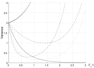
Figure 2: The variance $\langle(X_{1}-X_{2})^{2}\rangle$ as a function of time for $\Gamma_{2}/\Gamma_{1}=0.2$ (pluses), $\Gamma_{2}/\Gamma_{1}=0.5$ (dot-dashed line), $\Gamma_{2}/\Gamma_{1}=1$ (solid line), $\Gamma_{2}/\Gamma_{1}=2$ (dotted line), and $\Gamma_{2}/\Gamma_{1}=3$ (dashed line). The coupling is taken to be ideal, i.e., $\epsilon=1$.

If $\Gamma_{2}/\Gamma_{1}\neq 1$ and/or $\epsilon<1$, then the variance $\langle(X_{1}-X_{2})^{2}\rangle$ attains a finite minimum value at a particular time, after which it increases indefinitely. Defining $\lambda=\Gamma_{2}/\Gamma_{1}$, this minimum value is calculated to be

$$\langle(X_{1}-X_{2})^{2}\rangle_{\rm min}=\frac{2}{(1+\lambda)^{2}}\left[\frac{(2\sqrt{\epsilon}\lambda^{\frac{3}{2}})^{\frac{1}{1+\lambda}}}{(1+\lambda-2\sqrt{\lambda\epsilon})^{\frac{1}{1+\lambda}-1}}+2\sqrt{\lambda\epsilon}\left(\frac{2\sqrt{\epsilon}\lambda^{\frac{3}{2}}}{1+\lambda-2\sqrt{\lambda\epsilon}}\right)^{\frac{-\lambda}{1+\lambda}}\right]^{2},$$ (36)

and the time at which the minimum value occurs is given by

$$\Gamma_{1}t_{\rm min}(\lambda)=\frac{1}{1+\lambda}\ln\left[\frac{2\lambda\sqrt{\lambda\epsilon}}{1+\lambda-2\sqrt{\lambda\epsilon}}\right].$$ (37)

Plots of $\langle(X_{1}-X_{2})^{2}\rangle_{\rm min}$ and $\Gamma_{1}t_{\rm min}$ versus $\lambda$ are shown in Figs. 3 and 4 for several values of $\epsilon$. Note that $t_{\rm min}>0$ only where $\lambda>1/(4\epsilon)$. If $\lambda<1/(4\epsilon)$ then there is no reduction in the variance below the vacuum level.

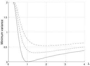
Figure 3: Minimum variance $\langle(X_{1}-X_{2})^{2}\rangle_{\rm min}$ as a function of $\lambda=\Gamma_{2}/\Gamma_{1}$ for $\epsilon=1$ (solid line), $\epsilon=0.9$ (dashed line) (minimum value of $0.30$ at $\lambda=1.46$), and $\epsilon=0.8$ (dot-dashed line) (minimum value of $0.54$ at $\lambda=1.95$).

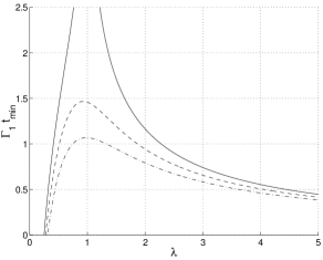
Figure 4: Time at which minimum variance occurs, $\Gamma_{1}t_{\rm min}$, as a function of $\lambda=\Gamma_{2}/\Gamma_{1}$ for $\epsilon=1$ (solid line), $\epsilon=0.9$ (dashed line), and $\epsilon=0.8$ (dot-dashed line).

From Figs. 3 and 4 (in particular, from their asymmetry about the point $\lambda=1$), it is clear that the scheme generally performs best in the regime where $\Gamma_{2}\geq\Gamma_{1}$ (i.e., $\lambda\geq 1$). In particular, significant reductions in the variances below the vacuum level occur over a broad region of $\Gamma_{2}$ values, provided $\Gamma_{2}\geq\Gamma_{1}$.

With decreasing values of the parameter $\epsilon$ (i.e., with decreasing coupling efficiency or increasing transmission losses), the minimum attainable variance increases and occurs for larger values of $\lambda$ and at somewhat earlier times. It follows that, for a realistic system with $\epsilon<1$, it would be advantageous to work in a regime with $\Gamma_{2}>\Gamma_{1}$. This is further illustrated in Fig. 5, where the variance is again plotted as a function of time, but now for several combinations of $\lambda$ and $\epsilon$. It is worth noting that a significant reduction in the variance ($\sim 73\%$) is still possible with $\epsilon=0.8$, i.e., $\langle(X_{1}-X_{2})^{2}\rangle_{\rm min}\simeq 0.54$ at $\Gamma_{1}t_{\rm min}\simeq 0.8$ for $\lambda=2$.

It should also be noted that, for the examples chosen in the regime where $\epsilon<1$ and $\lambda\geq 1$, the minimum variance generally occurs at times $\Gamma_{1}t$ of the order of 1. The mean excitation number for motional mode 1, $\langle b_{1}^{\dagger}b_{1}\rangle$, is then of the order of $e^{2}-1\simeq 6$, with a slightly smaller value for $\langle b_{2}^{\dagger}b_{2}\rangle$.

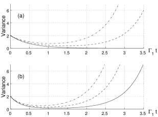
Figure 5: Variance $\langle(X_{1}-X_{2})^{2}\rangle$ as a function of time for (a) $\lambda=1$ and (b) $\lambda=2$, with $\epsilon=1$ (solid line), $\epsilon=0.9$ (dashed line), and $\epsilon=0.8$ (dot-dashed line).

V Comparison With Numerical Calculations

Starting from the master equation (13), which includes the cavity dynamics, a closed set of differential equations can be obtained for various correlation functions of the system. We have integrated these equations numerically (using a 4th-order Runge-Kutta method) and computed the variance $\langle(X_{1}-X_{2})^{2}\rangle$ for comparison with the results of the adiabatic approximation. This comparison is presented in Figs. 6 and 7 for several example sets of parameters.

On the timescales shown, the adiabatic approximation is seen to work well provided the coupling strengths $\Omega_{j}$ are, roughly, at least five to ten times smaller than the cavity decay rates $\kappa_{j}$. For larger values of $\Omega_{j}$ the maximum degree of reduction in the variance is significantly reduced and the dynamics obviously become somewhat more complicated, e.g., oscillatory behaviour starts to feature and excitation of the cavity modes increases.

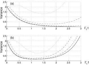
Figure 6: Comparison of numerical and adiabatic approximation results for $\langle(X_{1}-X_{2})^{2}\rangle$ versus time with $\kappa_{1}=\kappa_{2}=1$. The adiabatic approximation is shown in each plot as a solid line. (a) $\lambda=1$, with $\Omega_{1}=\Omega_{2}=0.1$ (dashed line), $\Omega_{1}=\Omega_{2}=0.2$ (dot-dashed line), $\Omega_{1}=\Omega_{2}=0.5$ (dotted line). (b) $\lambda=2$, with $\Omega_{1}=0.1$, $\Omega_{2}=\sqrt{2}\times 0.1$ (dashed line), $\Omega_{1}=0.2$, $\Omega_{2}=\sqrt{2}\times 0.2$ (dot-dashed line), $\Omega_{1}=0.5$, $\Omega_{2}=\sqrt{2}\times 0.5$ (dotted line).

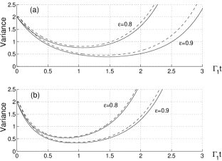
Figure 7: Comparison of numerical and adiabatic approximation results for $\langle(X_{1}-X_{2})^{2}\rangle$ versus time with $\kappa_{1}=\kappa_{2}=1$ and nonideal coupling between the cavities (i.e., $\epsilon<1$). The adiabatic approximation is shown in each plot as a solid line. (a) $\lambda=1$, with $\Omega_{1}=\Omega_{2}=0.1$ (dashed lines). (b) $\lambda=2$, with $\Omega_{1}=0.1$, $\Omega_{2}=\sqrt{2}\times 0.1$ (dashed lines).

VI Practical Considerations

We now consider in slightly more detail the conditions under which the most significant assumptions required by our model should be satisfied. Firstly though, as a more general comment, we note that exciting progress has been made recently in experimental cavity QED with single trapped atoms or ions Ye99 ; Hoo00 ; Pin00 ; Gut01 ; Mun02 . In fact, various “ingredients” of the scheme presented in this work have already been demonstrated.

VI.1 Trap Frequency

The neglect of terms in the effective motion-cavity mode interaction Hamiltonians which vary like $e^{\pm 2i\nu_{j}t}$ requires that the trap frequencies be large in comparison with the cavity decay rates $\kappa_{j}$ and the effective coupling parameters $\Omega_{j}$. To quantify this a little more precisely, previous numerical studies have shown that this rotating-wave approximation is very good provided the trap frequencies are at least an order of magnitude larger than $\kappa_{j}$ and $\Omega_{j}$ Parkins99 ; Parkins01 . We note that an experimental situation with $\nu_{j}\gg\kappa$ has been realized recently with single calcium ions trapped inside a high-finesse optical cavity Mun02 .

VI.2 Lamb-Dicke Approximation

The Lamb-Dicke approximation has been examined in some detail in Parkins01 . Taking into account the spread of the phonon number distribution associated with a general state, a condition for the validity of this approximation can be derived as

$$\frac{1}{2}\eta_{x}^{2}\left(1+\bar{n}_{x}+a\sigma_{\bar{n}_{x}}\right)\ll 1,$$ (38)

where $\bar{n}_{x}$ is the mean phonon number, $\sigma_{\bar{n}_{x}}^{2}$ is the variance of the number state distribution, and $a\sim 2-3$ (i.e., a few standard deviations from the mean). If we assume that the number state distribution of each mode is close to that of a thermal mode, then we can take $\sigma_{\bar{n}_{x}}\simeq(\bar{n}_{x}^{2}+\bar{n}_{x})^{1/2}\simeq\bar{n}_{x}+1/2$ for $\bar{n}_{x}>2$, and, with $a=3$, the condition becomes

$$\bar{n}_{x}\ll\frac{1}{2\eta_{x}^{2}}-\frac{5}{8}.$$ (39)

For $\eta_{x}=0.1$ this reduces to $\bar{n}_{x}\ll 49$. As noted earlier, at the time when minimum variances are generally achieved by our scheme (e.g., with $\epsilon<1$ and $\lambda\geq 1$), the mean phonon excitation numbers are of the order of 5–6, suggesting that Lamb-Dicke parameters of the order of 0.1 or smaller are sufficient.

Such values of the Lamb-Dicke parameter have been achieved with single atoms in cavity QED settings Ye99 ; Gut01 ; Mun02 . An ability to position the trap center very precisely at any point along the cavity standing wave field (e.g., at a node of the field, as required by the present scheme) has also been demonstrated Gut01 ; Mun02 .

Before continuing, we briefly mention the further interesting possibility of introducing a nontrivial time dependence to one or both of the coupling laser fields. One such example is illustrated in Fig. 8. Here, $\Omega_{2}=1$ (in dimensionless units) is fixed, while $\Omega_{1}(t)=\Omega_{2}\sin(t/\tau)$ ($\tau=20,25,30$), i.e., the effective parametric coupling strength is slowly increased from zero in the first atom-cavity system. If we consider the point for each case at which the variance is reduced to 0.2 (i.e., a 90% reduction below the “vacuum” level), then the corresponding mean phonon number at this time is seen to be only of the order of 2–3 for time-dependent $\Omega_{1}(t)$, whereas for the case of constant $\Omega_{1}$ and $\Omega_{2}$ (also shown in the figures) a variance of 0.2 is only attained with a mean phonon number greater than 10.

We have not explored other time dependencies in detail, but it would appear that there could be some advantage to doing so, in particular, from the point of view of minimizing the variance while maintaining mean phonon excitation numbers which comfortably satisfy the Lamb-Dicke constraint.

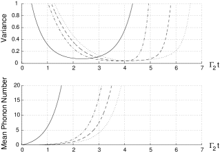
Figure 8: Variance $\langle(X_{1}-X_{2})^{2}\rangle$ and mean phonon number $\langle b_{1}^{\dagger}b_{1}\rangle$ as a function of time from numerical simulation of Eq. (13) using $\epsilon=1$, $\kappa_{1}=\kappa_{2}=10$, $\Omega_{2}=1$ ($\Gamma_{2}=\Omega_{2}^{2}/\kappa_{2}=0.1$), and $\Omega_{1}(t)=\Omega_{2}\sin(t/20)$ (dot-dashed line), $\Omega_{1}(t)=\Omega_{2}\sin(t/25)$ (dashed line), $\Omega_{1}(t)=\Omega_{2}\sin(t/30)$ (dotted line). The case $\Omega_{1}=\Omega_{2}=1$ is shown as a solid line.

VI.3 Atomic Spontaneous Emission

In practice, finite excitation of the atomic excited state will introduce the effects of spontaneous emission to the dynamics. Random momentum recoils associated with spontaneous emission events will disturb the motional states in an uncontrollable manner. However, if the rate at which such events occur is small compared with the rate at which the entangled states of interest are prepared by our scheme, then the effects of spontaneous emission can essentially be neglected.

In Parkins01 the rate of spontaneous emission events affecting the motional state is estimated for the kind of configuration we are considering here. By comparing this rate with the rates $\Gamma_{i}$, which characterize the preparation of the entangled motional states, the general condition under which the effects of spontaneous emission can be neglected is derived to be

$$\frac{10g_{0}^{2}}{\kappa\gamma}\gg 1,$$ (40)

where $\gamma$ is the linewidth (FWHM) of the internal atomic excited state. This is basically the condition of strong-coupling cavity QED, as realized, for example, in the single-atom experiments of Ye99 ; Hoo00 ; Pin00 (where values of $g_{0}^{2}/(\kappa\gamma)$ in the range 30–150 were achieved).

Finally, note that throughout this work we have neglected any forms of motional state decoherence associated with the trap itself. This seems reasonable, at least in the case of trapped ions, where typical timescales for motional decoherence and heating observed in recent experiments are of the order of milliseconds or longer Roos99 ; Turchette00 . With values of $g_{0}$ and $\kappa$ in the MHz range, we would anticipate a timescale for preparation of the motional states (i.e., $\Gamma_{i}^{-1}$) that is more than an order of magnitude shorter than such decoherence times.

VII Conclusions

In conclusion, we have described a scheme for entangling motional and light-field modes via an effective parametric (or two-mode squeezing) interaction realized in a single-atom cavity QED setting. Through decay of the cavity field through one of its mirrors, the cavity field entanglement is transferred to an external propagating field which may be coupled to the motional mode of a distant atom via a second cavity-QED-mediated interaction. This enables the preparation of an EPR-type entangled state of the position and momentum variables of separated atoms. This has a distinct advantage over a related scheme Parkins00a for preparing such a state in that a separate source of entangled light beams is not required.

We have given consideration to various practical issues associated with the scheme and pointed to a variety of recent experiments in single-atom cavity QED which collectively offer great encouragement to our proposal. Realization of the scheme would offer the exciting possibility of implementing a variety of continuous variable quantum computation and communication protocols, as well as opening the door to further investigations of fundamental aspects of entangled quantum systems, only now with distantly-separated massive particles Parkins00a .

- (1) L. Vaidman, Phys. Rev. A 49, 1473 (1994).
- (2) S. L. Braunstein and H. J. Kimble, Phys. Rev. Lett. 80, 869 (1998).
- (3) A. Furusawa et al., Science 282, 706 (1998).
- (4) T. C. Ralph, Phys. Rev. A 61, 010303(R) (2000).
- (5) M. Hillery, Phys. Rev. A 61, 022309 (2000).
- (6) S. F. Pereira, Z. Y. Ou, and H. J. Kimble, Phys. Rev. A 62, 042311 (2000).
- (7) M. D. Reid, Phys. Rev. A 62, 062308 (2000).
- (8) M. Ban, J. Opt. B: Quantum Semiclass. Opt. 1, L9 (1999).
- (9) S. L. Braunstein and H. J. Kimble, Phys. Rev. A 61, 042302 (2000).
- (10) X. Li et al., Phys. Rev. Lett. 88, 047904 (2002).
- (11) S. Lloyd and S. L. Braunstein, Phys. Rev. Lett. 82, 1784 (1999).
- (12) M. D. Lukin, S. F. Yelin, and M. Fleischhauer, Phys. Rev. Lett. 84, 4232 (2000).
- (13) A. Mair et al., Phys. Rev. A 65, 031802 (2002).
- (14) A. V. Turukhin et al., Phys. Rev. Lett. 88, 023602 (2002).
- (15) A. S. Zibrov et al., Phys. Rev. Lett. 88, 103601 (2002).
- (16) A. E. Kozhekin, K. Mølmer, and E. Polzik, Phys. Rev. A 62, 033809 (2000).
- (17) L.-M. Duan, J. I. Cirac, P. Zoller, and E. S. Polzik, Phys. Rev. Lett. 85, 5643 (2000).
- (18) B. Julsgaard, A. Kozhekin, and E. S. Polzik, Nature 413, 400 (2001).
- (19) A. S. Parkins and H. J. Kimble, J. Opt. B: Quantum Semiclass. Opt. 1, 496 (1999).
- (20) A. S. Parkins and H. J. Kimble, Phys. Rev. A 61, 052104 (2000).
- (21) A. S. Parkins and H. J. Kimble, in Frontiers of Laser Physics and Quantum Optics, Proceedings of the International Conference on Laser Physics and Quantum Optics, edited by Z. Xu, S. Xie, S.-Y. Zhu, and M. O. Scully (Springer, Berlin, 2000), p. 321. See also quant-ph/9909021.
- (22) A. S. Parkins and E. Larsabal, Phys. Rev. A 63, 012304 (2001).
- (23) S. Mancini and S. Bose, Phys. Rev. A 64, 032308 (2001).
- (24) A. Einstein, B. Podolsky, and N. Rosen, Phys. Rev. 47, 777 (1935).
- (25) Z. Y. Ou, S. F. Pereira, H. J. Kimble, and K. C. Peng, Phys. Rev. Lett. 68, 3663 (1992).
- (26) Z. Y. Ou, S. F. Pereira, and H. J. Kimble, Appl. Phys. B: Photophys. Laser Chem. 55, 265 (1992).
- (27) H. Zeng and F. Lin, Phys. Rev. A 50, R3589 (1994).
- (28) C. W. Gardiner, Phys. Rev. Lett. 70, 2269 (1993).
- (29) H. J. Carmichael, Phys. Rev. Lett. 70, 2273 (1993).
- (30) P. Kochan and H. J. Carmichael, Phys. Rev. A 50, 1700 (1994).
- (31) C. W. Gardiner and A. S. Parkins, Phys. Rev. A 50, 1792 (1994).
- (32) C. W. Gardiner and P. Zoller, Quantum Noise (Springer, Berlin, 2000).
- (33) J. Ye, D. Vernooy, and H. J. Kimble, Phys. Rev. Lett. 83, 4987 (1999).
- (34) C. J. Hood et al., Science 287, 1447 (2000).
- (35) P. W. H. Pinkse, T. Fischer, P. Maunz, and G. Rempe, Nature 404, 365 (2000).
- (36) G. R. Guthöhrlein et al., Nature 414, 49 (2001).
- (37) A. B. Mundt et al., preprint, quant-ph/0202112.
- (38) Ch. Roos et al., Phys. Rev. Lett. 83, 4713 (1999).
- (39) Q.A. Turchette et al., Phys. Rev. A 61, 063418 (2000).