Phase estimation as a quantum nondemolition measurement

Abstract

The phase estimation algorithm, which is at the heart of a variety of quantum algorithms, including Shor’s factoring algorithm, allows a quantum computer to accurately determine an eigenvalue of an unitary operator. Quantum nondemolition measurements are a quantum mechanical procedure, used to overcome the standard quantum limit when measuring an observable. We show that the phase estimation algorithm, in both the discrete and continuous variable setting, can be viewed as a quantum nondemolition measurement.

There is currently a great deal of active research aimed at developing implementation schemes for quantum computation. For an overview of this field see Nielsen and Chuang Nielsen and Chuang (2000) or Preskill notes Preskill (1998) and references therein. The goal of quantum computation is to build a computer, which, using the laws of quantum mechanics, can out perform any classical computer. Using the laws of quantum mechanics to enhance a device’s performance is not new. In quantum optics, the procedure of quantum nondemolition (QND) measurement Caves et al. (1980); Milburn and Walls (1983); LaPorta et al. (1989); Holland et al. (1990); Poizat and Grangier (1993) aims to accurately measure an observable without perturbing it. This procedure is consistent with the uncertainty principle, as, ideally, noise is induced only in the conjugate of the observable being measured.

Much of the impetus for research in quantum computation stems from Shor’s algorithm Shor (1994), which allows a quantum computer to factor integers exponentially faster than can currently be done on a classical computer. The factoring of large integers allows the decryption of many public key encryption systems. It has been shown that Shor’s, and many other quantum algorithms, can be described in terms of the phase estimation algorithm Kitaev ; Cleve et al. (1998).

It is evident that both phase estimation and QND measurement have the same goal: they both aim to accurately measure the eigenvalue of an operator (observable). In this paper we show that they are essentially the same procedure. That is, every instance of the phase estimation algorithm can be considered a QND measurement.

The original motivation for the study of QND measurements was the need to accurately measure weak classical forces Caves et al. (1980). Such measurements will be necessary, for example, in the detection of gravitational radiation. Classically, it is possible to measure both the position and momentum of a particle with complete precision. However, quantum mechanics tells us that the product of the uncertainty in the position and momentum of a particle must be greater than Planck’s constant divided by $4\pi$,

$$\Delta x\Delta p \geq \frac{\hbar}{2}.$$ (1)

The consequence of the uncertainty principle for an oscillator is the fact that any quantum mechanical state is characterized by an “error box” in the phase plane with area at least

$$\Delta x\Delta p/m\omega \geq \hbar/2m\omega,$$ (2)

where $m$ and $\omega$ are the mass and angular frequency respectively Caves et al. (1980). We can re-write Eq. (2) in terms of the quadrature variables, $\hat{X}$ and $\hat{Y}$,

$$\Delta X\Delta Y \geq \hbar/2m\omega,$$ (3)

where

$$\hat{x}+i\hat{p}/m\omega = (\hat{X}+i\hat{Y})e^{-i\omega t}.$$ (4)

If we naïvely perform an amplitude-and-phase measurement of the quadrature variables, we obtain a round error box, with

$$\Delta X=\Delta Y = \sqrt{\frac{\hbar}{2m\omega}}.$$ (5)

However, by performing a back-action-evading QND measurement of, say, $\hat{X}$, the error box becomes a long thin ellipse, with

$$\Delta X\ll\Delta Y$$ (6)

and $\Delta X$ can be made as small as one wishes, in principle.

Although a precise definition for a QND measurement is hard to pin down from the literature, there are three basic criteria which a QND measurement must satisfy. Firstly, it is required that the QND variable $\hat{A}$, which we wish to measure, commutes with the free Hamiltonian evolution of the system,

$$\begin{array}[]{lcr}&[\hat{H}_{F},\hat{A}]=0,&\hskip 56.9055pt\mbox{(QND 1)}\end{array}$$

so that if the system is measured in an eigenstate of $\hat{A}$, it remains in this eigenstate for all subsequent times, (perhaps only in the interaction picture). The most important criterion which must be satisfied, is that the Hamiltonian, $\hat{H}_{SM}$, coupling the meter variable $\hat{B}$ to the system must commute with the QND variable $\hat{A}$,

$$\begin{array}[]{lcr}&[\hat{H}_{SM},\hat{A}]=0.&\hskip 56.9055pt\mbox{(QND 2)}\end{array}$$

This is known as the back action evasion criterion. Finally, it is also necessary that the meter variable $\hat{B}$, does not commute with the interaction Hamiltonian,

$$\begin{array}[]{lcr}&[\hat{H}_{SM},\hat{B}]\neq 0.&\hskip 56.9055pt\mbox{(QND 3)}\end{array}$$

If this requirement is not fullfilled, then measuring the meter variable $\hat{B}$ will yield no information about the QND variable $\hat{A}$.

To illustrate how a QND measurement procedure works, consider the example of an ideal quadrature phase measurement of a single mode field Walls and Milburn (1995). Suppose we have two degenerate modes $a$ and $b$, of an electromagnetic field. We wish to measure $\hat{X}_{a}$ using the meter variable $\hat{X}_{b}$. Now, if we assume that the amplitude quadratures of each mode can be coupled according to the interaction Hamiltonian,

$$\hat{H}_{SM} = \hbar\chi\hat{X}_{a}\hat{Y}_{b},$$ (7)

where $\chi$ is the coupling strength, then clearly (QND 2) and (QND 3) are satisfied. (QND 1) is also satisfied by choosing a rotating frame of reference. In order to draw analogies with the phase estimation algorithm, we will divide the QND measurement into three steps. The first step involves initializing mode $b$ into the zero eigenstate of the meter variable, $|0\rangle_{b}$,

$$\hat{X}_{b}|0\rangle_{b} = 0.$$ (8)

Now, for simplicity, we will assume that mode $a$ is already in an eigenstate $|x\rangle_{a}$ of the QND variable,

$$\hat{X}_{a}|x\rangle_{a} = x|x\rangle_{a}.$$ (9)

Thus, the initial state of the quantum system is

$$|x\rangle_{a}|0\rangle_{b}.$$ (10)

Re-writing the meter system in terms of the phase variable, $\hat{Y}_{b}$, gives

$$\int\!\!dy\ |x\rangle_{a}|y\rangle_{b}.$$ (11)

Evolving according to the interaction Hamiltonian (Eq. (7)) results in the state

$$e^{i\chi\hat{X}_{a}\hat{Y}_{b}}\int\!\!dy\ |x\rangle_{a}|y\rangle_{b} = \int\!\!dy\ e^{i\chi xy}|x\rangle_{a}|y\rangle_{b}.$$ (12)

Finally re-writing mode $b$ in terms of the amplitude variable $\hat{X}_{b}$, we have

$$|x\rangle_{a}|\chi x\rangle_{b}.$$ (13)

Therefore, by performing a quadrature measurement of the amplitude of mode $b$, we obtain information about the state of mode $a$.

In the above description we have used eigenstates of the quadrature variables, however, like position and momentum eigenstates, these are physically unrealisable. However, they can be approximated to arbitrary degree by using highly squeezed states.

The goal of the phase estimation algorithm is to obtain an eigenvalue of a unitary operator $\hat{U}$. Although hybrid systems have been discussed in the literature Travaglione and Milburn (2001); Lloyd (2000), generally the phase estimation algorithm is described in terms of (discrete) qubit registers Kitaev ; Cleve et al. (1998). Discrete classical computation, is accomplished through the manipulation of binary digits (bits) using logic gates such as AND, OR, NOT and FANOUT, whereas discrete quantum computation uses arrays of two level quantum systems (qubit registers) which are manipulated via one and two qubit unitary operators. In analogy with the classical bit, it is conventional to use the symbols $|0\rangle$ and $|1\rangle$ to denote the two levels of the quantum system. Also in analogy with classical computation, we use the compact integer representation to represent the basis states of a qubit register. For example,

$$|1\rangle_{3}\otimes|1\rangle_{2}\otimes|0\rangle_{1}\otimes|1\rangle_{0} \equiv |13\rangle.$$ (14)

For an $m$ qubit register, we also introduce the Hermitian operator,

$$\hat{\Lambda} = \sum_{j=0}^{m-1}I\otimes\cdots\otimes I\otimes\underbrace{2^{j-1}(I-Z)}_{j^{\mathrm{th}}\ \mathrm{term}}\otimes I\otimes\cdots\otimes I,$$ (15)

where $I$ is the identity operator, and $Z$ is the pauli operator, with matrix representation,

$$Z = \left[\begin{array}[]{rr}1&0\\ 0&-1\end{array}\right].$$ (18)

The computational basis states are eigenstates of the operator $\hat{\Lambda}$ with an eigenvalue corresponding to their integer representation,

$$\hat{\Lambda}|x\rangle = x|x\rangle\quad\forall\ x\in[0,1,\dots,2^{m}-1].$$ (19)

Another basis which is useful in understanding the phase estimation algorithm is the Fourier transformed (FT) basis. This is the basis which arises by performing the quantum Fourier tranformCoppersmith (1994), $\hat{Q}$, on the computational basis,

$$|\bar{x}\rangle\equiv\hat{Q}|x\rangle\quad\forall\ x\in[0,1,\dots,2^{m}-1].$$ (20)

The Hermitian operator associated with this basis is

$$\hat{\Gamma} = \hat{Q}\hat{\Lambda}\hat{Q}^{-1},$$ (21)

as

$$\hat{\Gamma}|\bar{x}\rangle = x|\bar{x}\rangle\quad\forall\ x\in[0,1,\dots,2^{m}-1].$$ (22)

Suppose that we have a register of qubits, the target register, which is in an eigenstate $|\phi\rangle_{T}$, of some unitary operator $\hat{U}$. We wish to determine the eigenvalue corresponding to $|\phi\rangle_{T}$. As $\hat{U}$ is unitary, we have

$$\hat{U}|\phi\rangle_{T} = e^{i\phi}|\phi\rangle_{T},$$ (23)

where $\phi$ is some number between 0 and $2\pi$. The phase estimation algorithm utilizes an auxillary register of qubits, which we shall call the index register. Fig. 1 depicts the quantum circuit diagram for the discrete phase estimation algorithm.

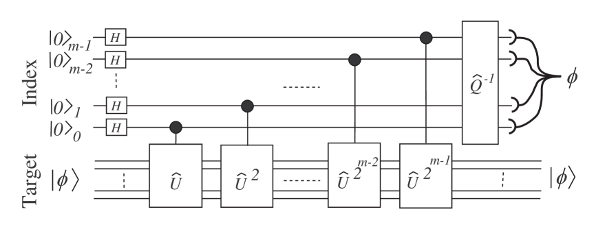
Figure 1: Quantum circuit diagram representing the discrete phase estimation algorithm.

The algorithm begins by placing the index register in the zero of the FT basis,

$$|\Phi_{0}\rangle = |\bar{0}\rangle_{I}|\phi\rangle_{T},$$ (24)

Assuming that each qubit in the index register begins the computation in the state $|0\rangle$, this step is accomplished by performing a Hadamard gate, $\hat{H}$, on each qubit. The next step is to perform a series of controlled $\hat{U}^{2^{k}}$ gates, which couple the target and index registers. For each $k\in[0,1,\dots,m-1]$, the gate $\hat{U}^{2^{k}}$ is applied conditionally upon the state of the $k$-th qubit in the index register. The cummulative effect of applying these gates is the operation, $\hat{U}^{\hat{\Lambda}}$. The state of the system after the application of $\hat{U}^{\hat{\Lambda}}$ is

$$|\Phi_{1}\rangle = \hat{U}^{\hat{\Lambda}}|\Phi_{0}\rangle$$ (25)

$$= \hat{U}^{\hat{\Lambda}}|\bar{0}\rangle_{I}|\phi\rangle_{T}$$

$$= \hat{U}^{\hat{\Lambda}}\frac{1}{\sqrt{M}}\sum_{j=0}^{M-1}|j\rangle_{I}|\phi\rangle_{T}$$

$$= \frac{1}{\sqrt{M}}\sum_{j=0}^{M-1}|j\rangle_{I}\hat{U}^{j}|\phi\rangle_{T}$$

$$= \frac{1}{\sqrt{M}}\sum_{j=0}^{M-1}|j\rangle_{I}e^{i\phi j}|\phi\rangle_{T},$$

where the last line makes use of Eq. (23). The final step in the algorithm involves measuring the index register in the FT basis, or equivalently, performing the operation $\hat{Q}^{-1}$, and measuring in the computational basis. This will, with high probability Travaglione and Milburn (2001), result in an $m$-bit approximation of $\phi$.

Having re-cast the phase estimation algorithm in terms of the FT basis, it is now not difficult to see that the phase estimation algorithm is effectively a QND measurement. We are trying to find an eigenvalue of the unitary operator, $\hat{U}$, which can of course be written as

$$\hat{U} \equiv e^{i\hat{H}_{U}},$$ (26)

for some Hermitian operator, $\hat{H}_{U}$. This operator is the QND variable that we are trying to measure, $\hat{\Gamma}$ is the meter variable, and $\hat{H}_{U}\hat{\Lambda}$ is the interaction Hamiltonian, as

$$\hat{U}^{\hat{\Lambda}} = e^{i\hat{H}_{U}\hat{\Lambda}}.$$ (27)

In the quantum circuit model, it is assumed that the qubits undergo no free evolution, so (QND 1) is automatically satisfied. It is clear from Eq. (27) that the back action evasion criterion is satisfied (QND 2), and it is not difficult to see that the interaction hamiltonian does not commute with the meter variable (QND 3) as

$$[\hat{\Lambda},\hat{\Gamma}] \neq 0.$$ (28)

To illustrate how the phase estimation algorithm acts as a QND measurement, we describe the simplest possible algorithm. Suppose we wish to determine the eigenvalue of the pauli $X$ operator, or NOT gate,

$$X = \left[\begin{array}[]{rr}0&1\\ 1&0\end{array}\right].$$ (31)

The eigenstates of this operator (ignoring a normalization factor) are $|0\rangle\pm|1\rangle$. The quantum circuit diagram for this simple phase estimation algorithm is depicted in Fig. 2.

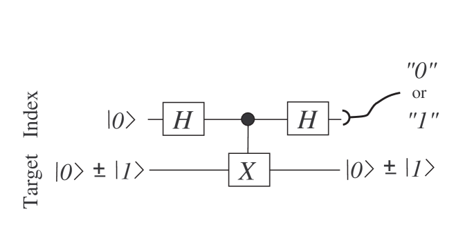
Figure 2: A simple example of the phase estimation algorithm

In this example the QND variable is

$$\hat{H}_{U} = \frac{\pi}{2}(I_{T}-X_{T}),$$ (32)

the meter variable is

$$\hat{\Gamma}=\hat{Q}\hat{\Lambda}\hat{Q}^{-1} = \frac{H_{I}(I_{I}-Z_{I})H_{I}}{2}=\frac{1}{2}\left[\begin{array}[]{rr}1&-1\\ -1&1\end{array}\right],$$ (35)

as the single qubit quantum Fourier transform is the self inverse Hadamard operator, $H_{I}$, and the interaction Hamiltonian is

$$\hat{H}_{U}\hat{\Lambda} = \frac{\pi}{4}(I_{T}-X_{T})(I_{I}-Z_{I}).$$ (36)

Obviously, all the QND criteria are satisfied, and the measurement proceeds by placing the meter system into the zero eigenstate of the meter variable, $|0\rangle+|1\rangle$, which is accomplished by the first Hadamard gate, evolving according to the interaction Hamiltonian, which is accomplished by the controlled NOT gate, and finally measuring the meter variable, by performing another Hadamard and then measuring in the computational basis.

We have just shown that the discrete phase estimation algorithm is equivalent to a QND measurement. Recently, a number of papers have been written exploring quantum computation using continuous variables Lloyd and Braunstein (1999); Gottesman et al. (2001); Ralph et al. (2001); Bartlett and Sanders (2001). We now show that continuous variable phase estimation is equivalent to continuous variable QND measurement.

As with all quantum algorithms, the phase estimation algorithm can be partitioned into three stages; the initialization stage, the entangling stage and the measurement stage. The initialization stage involves placing the index system into the zero eigenstate of the FT basis. The entangling stage involves the application of the operator

$$\hat{U}^{\hat{\Lambda}} = e^{i\hat{H}_{U}\hat{\Lambda}},$$ (37)

and the measurement stage involves measuring the index system in the conjugate of the computational basis. If we replace the discrete qubit registers with infinite level (continuous) quantum variables, and carry out each of these steps, we obtain something very similar to the ideal quadrature QND measurement discussed earlier. Suppose that the continuous variable operator, acting on the target system, whose eigenvalue we wish to determine is $e^{i\hat{A}_{T}}$, and we choose the position of the continuous index system as the computational basis. Then following the steps of the phase estimation algorithm, we prepare our index system in the zero eigenstate of the conjugate basis, that is, the zero momentum eigenstate. This step corresponds to initialising our meter variable. Then we perform the $\hat{U}$ operator, conditioned upon the computational basis, $e^{i\hat{x}_{I}\hat{A}_{T}}$, which corresponds to applying an interaction Hamiltonian which satisfies (QND 1) and (QND 2). Before finally performing a Fourier transform and measuring the position variable, which is equivalent to measuring the momentum of the index system (i.e. the meter variable). This is clearly a QND measurement of $\hat{A}$.

Of course, position eigenstates are physically unrealisable, and any continuous variable implementation of the phase estimation algorithm would need to be done using approximate position eigenstates, such as squeezed states. Just as ideal QND measurements can only be approximated experimentally, ideal continuous variable phase estimation can also only be approximated.

The study of quantum computation brings together a number of disciplines including computer science, mathematics and quantum mechanics. We have taken the phase estimation algorithm, which has its roots in computer science, and shown that it is equivalent to the quantum mechanical procedure of QND measurement. We have also described a continuous variable version of the phase estimation algorithm. It is interesting to speculate on whether other algorithms such as Grover’s algorithm might have similarities with well studied quantum phenomenon.