Theory for the optimal control of time-averaged quantities in open quantum systems

Abstract

We present variational theory for optimal control over a finite time interval in quantum systems with relaxation. The corresponding Euler-Lagrange equations determining the optimal control field are derived. In our theory the optimal control field fulfills a high order differential equation, which we solve analytically for some limiting cases. We determine quantitatively how relaxation effects limit the control of the system. The theory is applied to open two level quantum systems. An approximate analytical solution for the level occupations in terms of the applied fields is presented. Different other applications are discussed.

The manipulation of quantum mechanical systems by using ultrashort time-dependent fields represents a challenging fundamental physical problem. In the last years, a considerable amount of experimental and theoretical work was concentrated on designing laser pulses having optimal amplitude and modulation. Thus the control of the quantum dynamics in various systems like atoms and molecules[3], quantum dots[4], semiconductors[5], superconducting devices[6] and Bose-Einstein condensate[7] was achieved.

Several theoretical studies, most of them using numerical optimization techniques, have shown that it is possible to construct optimal external fields (e.g. laser pulses) to drive a certain physical quantity, like the population of a given state, to reach a desired value at a given time[8, 9, 10].

Although this kind of control might be relevant for many purposes, a more detailed manipulation of real systems may require the control of physical quantities over a finite time interval. The search for optimal fields able to perform such control is a much more challenging problem for which no theoretical description has been given so far.

In this letter we present for the first time an analytical theory for the control of simple open systems over a finite time interval. By applying a variational approach we derive a high-order differential equation from which the optimal control fields are obtained. We also determine the influence of relaxation, the limits of this control and its potential applications to the manipulation of fundamental physical quantities, like the induced current through impurities in semiconductors or the population of electronic states at metallic surfaces.

Our goal is to formulate a theory which permits to derive explicit equations to be satisfied by the optimal control field. Note that one can guess the form of such equations from general physical arguments. Since memory effects are expected to be important, one should search for a differential equation containing both the pulse area $\theta(t)=\int_{t_{0}}^{t}dt^{\prime}V(t^{\prime})$, where $V(t)$ is the external field envelope, and its time derivatives. Therefore, for the case of optimal control of dynamical quantities at a given time $t_{0}$, the differential equation satisfied by $\theta(t)$ must be of at least second order to fulfill the initial conditions $\theta(t_{0})$, $\dot{\theta}(t_{0})$. In the same way, the control of time averaged quantities over a finite time interval $[t_{0},t_{0}+T]$ with boundary conditions requires a differential equation of at least forth order for $\theta(t)$ due to the boundary conditions for $\theta(t)$ and $\dot{\theta}(t)$ at $t_{0}$ and $t_{0}+T$. We show below that for certain open systems a forth order differential equation for the control fields arises naturally using variational approach as an Euler-Lagrange (EL) equation.

We start by considering a quantum-mechanical system which is in contact with the environment and interacting with an external field $E(t)=V(t)\cos(\omega t)$. Here $V(t)$ refers to an arbitrary pulse and $\omega$ is the carrier frequency. The evolution of such system obeys the quantum Liouville equation for the density matrix $\rho(t)$ with dissipative terms. The control of a time averaged dynamical quantity of the system requires the search for the optimal shape $V(t)$ of the external field.

Thus, in order to obtain the optimal $V(t)$ on time interval $[0,T]$ we propose the following Lagrangian (throughout the paper we use atomic units $\hbar$=m=e=1)

$$L = \int_{0}^{T}{A(t)\Big{(}\frac{\partial}{\partial t}+i\hat{\cal{Z}}(t)\Big{)}\rho(t)dt}\,+\,\beta\int_{0}^{T}{{\cal{L}}_{1}dt}.$$ (1)

$\beta$ is a Lagrange multiplier and $A(t)$ is a Lagrange multiplier density. The first term in Eq. (1) ensures that the density matrix satisfies the quantum Liouville equation with the corresponding Liouville operator $\hat{\cal{Z}}(t)$[8]. While the first term describes the dynamics of the system under the external field, the functional ${\cal{L}}_{1}$ explicitly includes the description of the optimal control and is given by

$${\cal{L}}_{1}(\rho,V)={\cal{L}}_{ob}(\rho)+\lambda{V}^{2}(t)+\lambda_{1}{\left(\frac{dV(t)}{dt}\right)}^{2},$$ (2)

where $\lambda$ and $\lambda_{1}$ are Lagrange multipliers. ${\cal{L}}_{ob}(\rho)$ refers to a physical quantity to be maximized during the control time. The second term represents a constraint on the total energy of the control field

$$2\int_{0}^{T}{E}^{2}(t)dt\approx\int_{0}^{T}{V}^{2}(t)dt=E_{0}.$$ (3)

The third term represents a further constraint on the properties of the pulse envelope. The requirement

$$\int_{0}^{T}{\left(\frac{dV(t)}{dt}\right)}^{2}dt\leq R,$$ (4)

where $R$ is a positive constant, excludes infinitely narrow or sharp step-like solutions, which cannot be achieved experimentally.

Assuming that the density matrix $\rho(t)$ depends only on $\theta(t)$ and time, one obtains an explicit expression for the functional ${\cal L}_{1}={\cal L}_{1}(\theta,\dot{\theta},\ddot{\theta},t)$. The corresponding extremum condition $\delta{{\cal L}_{1}}=0$ yields the high-order EL equation

$$-\lambda_{1}\frac{d^{4}\theta}{{dt}^{4}}+\lambda\frac{d^{2}\theta}{{dt}^{2}}-\frac{1}{2}\frac{\partial{\cal L}_{ob}(\rho)}{\partial{\theta}}=0.$$ (5)

In order to solve Eq. (5) one can assume the natural boundary conditions $\theta(0)={\dot{\theta}}(0)={\dot{\theta}}(T)=0$, $\theta(T)=\theta_{T}$, which also ensure that $V(0)=V(T)=0$. The choice of the constant $\theta_{T}$ depends on the problem. In general, the constants $\theta_{T}$, $R$ and $E_{0}$ can be also object of the optimization. Note, that above formulated problem is highly nonlinear with respect to the function $\theta(t)$ and can be solved only numerically.

Eq. (5) is the central result of this letter and provides an explicit differential equation for the control field. Note that this equation is only applicable if $\rho=\rho(\theta(t),t)$.

In order to show that Eq. (5) can describe optimal control in real physical situations, we apply our theory to an open two level quantum system. This is characterized by the energy levels $\epsilon_{1}$ and $\epsilon_{2}$, a dipole matrix element $\mu$ and the longitudinal and transverse relaxation constants, $\gamma_{1}$ and $\gamma_{2}$, respectively. The carrier frequency of the control field is chosen to be the resonant frequency $\omega=\epsilon_{2}-\epsilon_{1}$. The dynamics of the density matrix $\rho(t)$ follows the equations (in the rotating wave approximation)

$$i\frac{\partial{\rho_{\ell\ell}}}{\partial{t}} = (-1)^{\ell}(\mu V(t)(\rho_{21}-\rho_{12})-i\gamma_{1}\rho_{22}),$$ (6)

$$i\frac{\partial{\rho_{12}}}{\partial{t}} = \mu V(t)(\rho_{22}-\rho_{11})-i\gamma_{2}\rho_{12},\;$$ (7)

with $\ell=1,2$. Note that $\rho_{11}+\rho_{22}=1$ and $\rho_{21}=\rho_{12}^{*}$. Eqs. (6) are used for the description of different effects, like for instance, the response of donor impurities in semiconductors to teraherz radiation[5], or the excitation of surface- into image charge states at noble metal surfaces[12]. Therefore, the initial conditions are set as $\rho_{11}=1,\rho_{22}=\rho_{12}=\rho_{21}=0$.

Eqs. (6) have the form $i\partial\rho(t)/\partial t={\hat{\tilde{\cal{Z}}}}{(t)}\rho{(t)}$ and are difficult to integrate, since $[{\hat{\tilde{\cal{Z}}}}(t),{\hat{\tilde{\cal{Z}}}}(t^{\prime})]\not=0$. However, the commutators $[{\hat{\tilde{\cal{Z}}}}(t),{\hat{\tilde{\cal{Z}}}}(t^{\prime})]$ become arbitrarily small under the condition[14]

$$\Big{|}\frac{\partial\log{V(t)}}{\partial t}\gamma_{\ell}\Big{|}\ll 1,\;$$ (8)

with $\ell=1,2$. In this case approximate solution for $\rho_{22}(t)$ is

$$\rho_{22}(t)=2\>\theta^{2}(t)F^{-1}\Big{(}1-\cosh(H)\exp(-(\gamma_{1}+\gamma_{2})t/2)$$ (9)

$$+(\gamma_{1}+\gamma_{2})t\>\sinh(H)\exp(-(\gamma_{1}+\gamma_{2})t/2)H^{-1}\Big{)},$$ (10)

where $H=\sqrt{((\gamma_{1}-\gamma_{2})^{2}t^{2}-16\;\theta^{2}(t))/2}$, and $F=\gamma_{1}\gamma_{2}t^{2}+4\;\theta^{2}(t)$. Note that this approximate solution becomes exact when $\gamma_{1}=\gamma_{2}=0$ or for a constant control field $V(t)=V_{0}$. The expression of Eq. (9) has the form $\rho=\rho(\theta(t),t)$ and therefore Eq. (5) is applicable.

Now we construct the functional ${\cal{L}}_{ob}(\rho)=\rho_{22}(t),$ so that the average occupation of the upper level $n_{2}=\int_{0}^{T}{\rho_{22}(t)dt}$ is maximized. Note, that $n_{2}$ proportional to the observed photocurrent[5] in teraherz experiments on semiconductors. The resonant tunneling current through an array of coupled quantum dots is also proportional to a such value[13].

We have calculated the optimal $V(t)$ from the numerical integration of Eq. (5) for different values of the relaxation constants $\gamma_{1}$ and $\gamma_{2}$ and of the energy $E_{0}$ and the curvature $R$ of the control fields. For simplicity we consider the control interval $[0,1]$.

In Fig. 1 we show the optimal field for an isolated ($\gamma_{1}=\gamma_{2}=0$) and for an open two level system for given values of the pulse energy and curvature. Note, that for both cases the pulse maximum occurs near the beginning of the control interval. This leads to a rapid increase of the population $\rho_{22}(t)$ and therefore to a maximization of $n_{2}$. In the case of an isolated system the pulse vanishes when the population inversion has been achieved, whereas for an open system the pulse must compensate the decay of $\rho_{22}(t)$ due to relaxation effects and remains finite over the whole control interval.

In the inset of Fig. 1 we show the corresponding dynamics of the population $\rho_{22}(t)$ for both cases. As mentioned before, Eq. (9) is exact for the isolated system. Note, that for the open system the analytical form of $\rho_{22}$ (Eq. (9)) compares well with the numerical solution of the Liouville equation. This indicates that $V(t)$ fulfills the condition(8) on the control interval.

We found that the value of $n_{2}$ increases both for the isolated and for the open system monotonously with energy of the optimal control field. In Fig. 2 we plot $n_{2}$ as a function of the energy $E_{0}$ and the curvature $R$ of the optimal fields obtained from Eq. (5). Note, that pulses of fixed shape (for instance Gaussian) would show an oscillating behavior for increasing energy due to Rabi oscillations [11]. The monotonous increase is a feature which characterizes the optimal pulses.

In order to achieve a simplified study of the physics contained in the control fields of Fig. 1, we analyze the problem in certain limiting cases. For instance, if $\gamma_{1,2}T\ll 1$ one can neglect decoherence within the control interval and Eq. (9) becomes $\rho_{22}(t)=\sin^{2}\left(\theta(t)\right)$. In order to make the problem analytically solvable, we reduce the order of the differential equation for the control fields. For that purpose we replace the constraint on the derivative of the field envelop (Eq. (4)) by a weaker one obtained from the condition

$$\int_{0}^{T}{\dot{\theta}}^{2}(t)dt-\frac{1}{T}{\left(\int_{0}^{T}\dot{\theta}(t)dt\right)}^{2}=\int_{0}^{T}{\cal{L}}_{w}(\theta)\geq S,$$ (11)

where S is a positive constant. Eq. (11) merely bounds the width of the envelope $V(t)$ in order to avoid unphysically narrow pulses. Thus, the Lagrangian density ${\cal{L}}_{1}$ for the optimal control has the form

$${\cal{L}}_{1}={\rho_{22}(t)}+\lambda\dot{\theta}^{2}(t)+\lambda_{2}{\cal{L}}_{w}(\theta),$$ (12)

while the corresponding EL equation is given by

$$2\lambda^{\prime}\ddot{\theta}(t)-\sin(2\>\theta(t))=0.$$ (13)

Note, that condition (11) only leads to a rescaling of the Lagrangian multiplier $\lambda$ to $\lambda^{\prime}=\lambda+\lambda_{2}$. The second order differential Eq. (13) requires two boundary conditions, for which we choose ${\theta}(0)=0$ and ${\theta}(T)=\pi/2$ (which ensure the population inversion). Eq. (13) resembles that for a mathematical pendulum and can be solved analytically. The resulting field envelope is given by

$$V(t)=V(0)\,dn(V(0)t,C),$$ (14)

where $dn$ is the Jacobian elliptic function, and $C=-{(\lambda^{\prime}V^{2}(0))}^{-1}$ is a constant of integration. Note, that $V(0)\not=0$. Using conditions (3) and (11) we determine coefficients $\lambda$ and $\lambda_{2}$. If we choose $C\to 1$ then we can obtain $V(T)\to 0$. In this case, Eq. (14) can be significantly simplified to $V(t)=\frac{\partial}{\partial t}{\arccos[2\exp{(V(0)t)}/(1+\exp{(2V(0)t)})]}.$

In Fig. 3 we plot the optimal control field $V(t)$ which maximizes the Lagrangian (12) for isolated and open two level systems. In both cases the field has its maximum value at $t=0$ and exhibits a monotonous decay. As in the case of the solutions of the forth-order Eq. (5) the control field is broader for the open system. In the inset of Fig. 3 we plot the population $\rho_{22}(t)$. The overall behavior of $\rho_{22}(t)$ is similar to that of the populations shown in Fig. 1.

It is important to point out, that a Lagrangian of the form of Eq. (12) always leads to a second order differential equation for the control fields as long as the condition $\rho=\rho(\theta(t),t)$ is satisfied. Therefore, one cannot demand extra boundary conditions for the fields $V(0)=V(T)=0$. Otherwise one would obtain the trivial solution $V(t)\equiv 0$, which is not consistent with either (3) or (11). Therefore, if conditions on $V(0)$ and $V(T)$ have to be imposed, a Lagrangian leading to a forth order differential equation is necessary, as we have shown before.

As it was mentioned before $n_{2}$ increases monotonously with the pulse energy for the optimal field. Since for the isolated system $n_{2}$ approaches the maximum possible value $n_{2}=T$, in the case of nonisolated systems there is a limit. In order to show that this limits is due to general physical reasons we analyze the occupation $\rho_{22}(t)$ (Eq. (9)) in more detail. For a strong control field satisfying $\gamma_{1,2}t/\theta(t)\ll 1$ the occupation $\rho_{22}(t)$ always lies under the curve $\rho_{22}^{max}(t)=(1+\exp(-(\gamma_{1}+\gamma_{2})t/2))/2$. This means that it exhibits an absolute upper bound. Therefore due to dissipative processes the following inequality holds for the controlled averaged value of $\rho_{22}$:

$$n_{2}=\int_{0}^{T}{\rho_{22}(t)dt}\leq T/2+(1-\exp(-(\gamma_{1}+\gamma_{2})T/2)/(\gamma_{1}+\gamma_{2}).$$ (15)

Eq. (15) shows the absolute limit for the optimal control of averaged occupations in open two level systems. In Fig. 4 we show the maximal possible value $\rho_{22}^{max}(t)$ and the time evolution of $\rho_{22}(t)$ induced by 40 randomly generated pulses (for some of which the condition $\gamma_{1,2}t/\theta(t)\ll 1$ is even not strictly fulfilled). From Fig. 4 we conclude that under the action of arbitrary control fields, the life time of the upper level cannot be longer than $2/(\gamma_{1}+\gamma_{2})$.

Using this result we can determine the maximal possible life-time for an image state at a Cu(111) surface which can be achieved by pulse shaping. According to Hertel et al.[12], those states are characterized by $\gamma_{1}=5\cdot 10^{13}s^{-1}$ and $\gamma_{2}=\gamma_{1}/2$. Thus, our theory predicts in that case an effective decay constant $\gamma_{eff}=(\gamma_{1}+\gamma_{2})/2=3.75\cdot 10^{13}s^{-1}$.

In summary, we presented a theory for the description of optimal control of time-averaged quantities in open quantum systems. In particular we have shown that the boundary conditions of the problem make a significant influence on the shape of the optimal fields. In contrast to other approaches our theory allows to derive an explicit differential equation for the optimal control field, which we integrated both numerically and exactly for some limiting cases. Our approximation $\rho(t)=\rho(\theta,t)$ was checked by direct integration of the Liouville equations and it seems to hold also in the case of strong relaxation. Using our theory we found the optimal fields which maximize the population of the upper levels of isolated and open two-level systems. We found an absolute upper bound for this kind of optimal control. Our approach can be used for further investigations, for instance,control of the dynamics of multi-level systems.

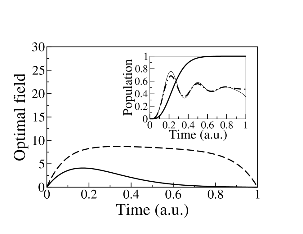
FIG. 1.: Optimal control field for an isolated two level system ($\gamma_{1,2}=0$, solid line). The pulse energy is $E_{0}=4.57$ and the pulse curvature $R=128.4$. The dashed line shows the optimal pulse for the open system ($\gamma_{1}=2\gamma_{2}=5$) with energy $E_{0}=53.54$ and curvature $R=808.8$. Inset: Dynamics of the occupation $\rho_{22}(t)$ for an isolated system (thick solid line) and with relaxation (dash dotted line-using formula (9), thin solid line-numerical solution of the Liouville equation (6)). Arbitrary units are used.

FIG. 2.: Dependence of the averaged occupation $n_{2}$ as a function of the energy $E_{0}$ and the curvature $R$ (see Eq. (4) ) of the optimal pulses.

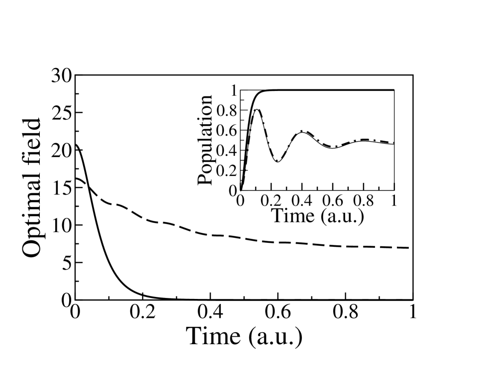
FIG. 3.: Optimal control field for an isolated two level system ($\gamma_{1,2}=0$, solid line). The pulse energy is $E_{0}=20.50$. Dashed line: optimal field for the open system ($\gamma_{1}=2\gamma_{2}=5$) with a pulse energy $E_{0}=89.72$. Inset: Dynamics of the occupation $\rho_{22}(t)$ for an isolated system (thick solid line) and with relaxation (dash dotted line using Eq. (9), thin solid line-numerical solution of the Liouville equation (6)).

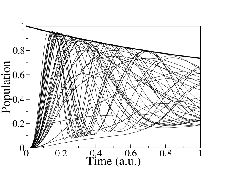
FIG. 4.: Dynamics of the occupation $\rho_{22}(t)$ for 40 randomly generated control pulses and for $\gamma_{1}=2\gamma_{2}=1$ (thin solid lines). The thick solid line represents a bound for the possible values of $\rho_{22}^{max}(t)=(1+\exp(-(\gamma_{1}+\gamma_{2})t/2))/2$.

REFERENCES

- [1] [‡] Corresponding author, garcia@physik.fu-berlin.de
- [2] [∗] grigoren@physik.fu-berlin.de
- [3] H.L. Haroutyunyan and G. Nienhuis, Phys. Rev. A 64, 033424 (2001). R. de Vivie-Riedle, K. Sundermann, Appl. Phys. B. 71, 285, (2000). C. Brif, H. Rabitz, S Wallentowitz, I.A. Walmsley, Phys. Rev. A 63, 063404, (2001).
- [4] P. Chen, C. Piermarocchi, and L.J. Sham, Phys. Rev. Lett. 87, 067401, (2001).
- [5] B.E. Cole et al, Nature (London), 410, 60 (2001).
- [6] Y. Nakamura, Yu.A. Pashkin and J.S. Tsai, Nature 398, 786 (1999).
- [7] S. Potting et al, Phys. Rev. A 64, 023604, (2001).
- [8] Y. Ohtsuki, W. Zhu and H. Rabitz, J. Chem. Phys. 110, 9825, (1999). S. G. Schirmer, M. D. Girardeau, J. V. Leahy, Phys. Rev. A 61, 012101 (2000).
- [9] Y. Ohtsuki et al. J. Chem. Phys. 114, 8867, (2001).
- [10] L. E. E. de Araujo, I. A. Walmsley, and C. R. Stroud.Jr. Phys. Rev. Lett. 81, 955,(1998).
- [11] O. Speer, M. E. Garcia and K. H. Bennemann, Phys. Rev. B 62, 2630 (2000).
- [12] T. Hertel, E. Knoesel, M. Wolf, and G. Ertl Phys. Rev. Lett. 76, 535 (1996).
- [13] T.H. Stoof and Yu. V. Nazarov, Phys. Rev. B 53, 1050 (1996).
- [14] further details will be published elswhere.