Experimental Implementation of Quantum Random Walk Algorithm

Abstract

The quantum random walk is a possible approach to construct new quantum algorithms. Several groups have investigated the quantum random walk and experimental schemes were proposed. In this paper we present the experimental implementation of the quantum random walk algorithm on a nuclear magnetic resonance quantum computer. We observe that the quantum walk is in sharp contrast to its classical counterpart. In particular, the properties of the quantum walk strongly depends on the quantum entanglement.

I Introduction

Since the discovery of the first two quantum algorithms, Shor’s factoring algorithm 1 and Grover’s database search algorithm 2 , research in the new born field of quantum computation exploded 3 . Mainly motivated by the idea that a computational device based on quantum mechanics might be (possibly exponentially) more powerful than a classical one 4 , great effort has been done to investigate new quantum algorithms and, more importantly, to experimentally construct a universal quantum computer. However, finding quantum algorithms is a difficult task. It has also been proved extremely difficult to experimentally construct a quantum computer, as well as to carry out quantum computations.

Recently, several groups have investigated quantum analogues of random walk algorithms 5 ; 6 ; 7 ; 8 ; 9 ; 10 , as a possible direction of research to adapt known classical algorithms to the quantum case. Random walks on graphs play an essential role in various fields of natural science, ranging from astronomy, solid-state physics, polymer chemistry, and biology to mathematics and computer science 11 . Current investigations show that quantum random walks have remarkably different features to the classical counterparts 5 ; 6 ; 7 ; 8 ; 9 ; 10 . The hope is that a quantum version of the random walk might lead to applications unavailable classically, and to construct new quantum algorithms. Indeed, the first quantum algorithms based on quantum walks with remarkable speedup have been reported al . Further, experimental schemes have also been proposed to implement such quantum random walks by using an ion trap quantum computer 9 and by using neutral atoms trapped in optical lattices 10 . Up to now, only three methods have been used to demonstrate quantum logical gates: trapped ions 12 , cavity QED 13 and NMR 14 . Of these methods, NMR has been the most successful with realizations of quantum teleportation 15 , quantum error correction 16 , quantum simulation 17 , quantum algorithms 18 , quantum games 19 and others 20 . In this paper, we present the experimental implementation of the quantum random walk algorithm on a two-qubit NMR quantum computer, and we believe it is the first experimental implementation of such quantum algorithms.

We consider continuous-time random walks (CTRW) 6 rather than discrete-time random walks 7 , on a circle with four nodes. We show that the evolution of this quantum walk is periodic and reversible, and yields an exactly uniform probability distribution at certain time. While the classical CTRW is irreversible and only approximates the uniform distribution at infinite-time limit. Further, we experimentally implement this quantum walk on a two-qubit quantum computer, using a unitary operator which has the right “effective” Hamiltonian, with good agreements between theory and experiment. It is interestingly found that the property of the quantum walk strongly depends on the entanglement between the two qubits. The uniform distribution could be obtained only when the two qubits are maximally entangled.

II Quantum CTRW on a Circle

The concept of quantum CTRW is proposed in Ref. 6 . On a circle with four nodes, we denote the set of nodes by $\left\{0,1,2,3\right\}$. Since the structure of the circle is periodic, only two nodes, $\left(k+1\right)\operatorname{mod}4$ and $\left(k-1\right)\operatorname{mod}4$, are connected to node $k$ $\left(k=0,1,2,3\right)$. In the classical CTRW, let $\gamma$ denote the jumping rate, which is a fixed, time-independent constant that represents the probability moving from a given node to a connected one per unit time. The generator matrix 6 of this walk can therefore be written as

$$H=\left(\begin{array}[c]{cccc}2\gamma&-\gamma&0&-\gamma\\ -\gamma&2\gamma&-\gamma&0\\ 0&-\gamma&2\gamma&-\gamma\\ -\gamma&0&-\gamma&2\gamma\end{array}\right).$$ (1)

Consider a particle walking classically on this circle, let $P_{k}^{C}\left(t\right)$ denote the probability of being at node $k$ at time $t$ (the superscript $C$ denotes “Classical”), then we have

$$\frac{d}{dt}P_{k}^{C}\left(t\right)=-\sum\nolimits_{l=0}^{3}H_{kl}P_{l}^{C}\left(t\right).$$ (2)

This equation conserves the probability in the sense that $\sum_{k=0}^{3}P_{k}^{C}\left(t\right)\equiv 1$.

A natural way to the quantum version of this CTRW is to construct a Hilbert space spanned by the four basis $\left\{\left|0\right\rangle,\left|1\right\rangle,\left|2\right\rangle,\left|3\right\rangle\right\}$, respectively corresponding to the four nodes $\left\{0,1,2,3\right\}$. The state of a particle walking quantum mechanically on this circle is then denoted by $\left|\psi\left(t\right)\right\rangle$, which is generally a superposition of the four basis, rather than classical mixing of the probabilities of being at the four nodes. The generator matrix in classical walks is now treated as the Hamiltonian of the quantum evolution 6 . Therefore the Schrödinger equation of the state $\left|\psi\left(t\right)\right\rangle$ is

$$\frac{d}{dt}\left\langle k\right|\left.\psi\left(t\right)\right\rangle=-i\sum\nolimits_{l=0}^{3}\left\langle k\right|H\left|l\right\rangle\left\langle l\right|\left.\psi\left(t\right)\right\rangle.$$ (3)

If measuring at time $t$, we can obtain a certain probability distribution on the circle. The probability of being at node $k$ is $P_{k}^{Q}\left(t\right)=\left|\left\langle k\right|\left.\psi\left(t\right)\right\rangle\right|^{2}$ (the superscript $Q$ denotes “Quantum”), and the conservation of probability is obviously guaranteed by the normalization $\left\langle\psi\left(t\right)\right|\left.\psi\left(t\right)\right\rangle\equiv 1$.

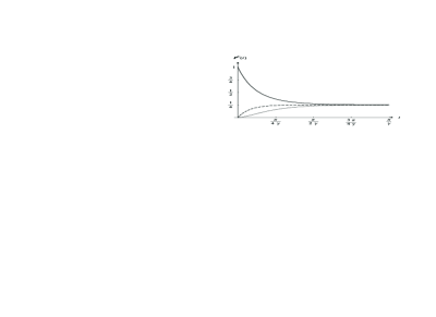
Figure 1: The probabilities of being at the four nodes in the classical version of this CTRW. The solid (dotted) line corresponds to $P_{0}^{C}\left(t\right)$ ($P_{2}^{C}\left(t\right)$). The dashed line corresponds to $P_{1}^{C}\left(t\right)$ and $P_{3}^{C}\left(t\right)$, since $P_{1}^{C}\left(t\right)=P_{3}^{C}\left(t\right)$.

Let the walking particle start from node $0$, it is then easy to find the probability of being at node $k$ at any time $t$ in both the classical walks and the quantum walks (by solving equations (2) and (3), respectively). The detailed calculation yields that for the classical walks the probabilities are

$$\left\{\begin{array}[c]{l}P_{0}^{C}\left(t\right)=\frac{1}{4}+\frac{1}{2}e^{-2\gamma t}+\frac{1}{4}e^{-4\gamma t}\\ P_{1}^{C}\left(t\right)=P_{3}^{C}\left(t\right)=\frac{1}{4}-\frac{1}{4}e^{-4\gamma t}\\ P_{2}^{C}\left(t\right)=\frac{1}{4}-\frac{1}{2}e^{-2\gamma t}+\frac{1}{4}e^{-4\gamma t}\end{array}\right..$$ (4)

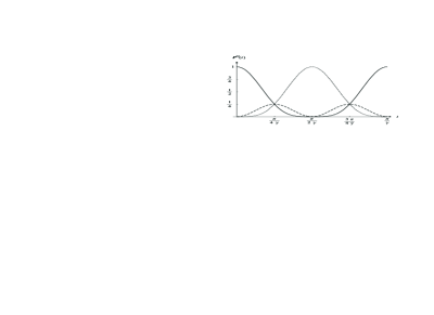
Figure 2: The probabilities of being at the four nodes in the quantum version of this CTRW. The solid (dotted) line corresponds to $P_{0}^{Q}\left(t\right)$ ($P_{2}^{Q}\left(t\right)$). The dashed line corresponds to $P_{1}^{Q}\left(t\right)$ and $P_{3}^{Q}\left(t\right)$, since $P_{1}^{Q}\left(t\right)=P_{3}^{Q}\left(t\right)$.

In the quantum case, the initial state of the particle is $\left|\psi\left(0\right)\right\rangle=\left|0\right\rangle$, from equation (3), we have

$$\left|\psi\left(t\right)\right\rangle =e^{-iHt}\left|0\right\rangle$$

$$=e^{-2i\gamma t}\cos^{2}\gamma t\left|0\right\rangle-e^{-2i\gamma t}\sin{}^{2}\gamma t\left|2\right\rangle$$

$$+\frac{i}{2}e^{-2i\gamma t}\sin 2\gamma t\left(\left|1\right\rangle+\left|3\right\rangle\right).$$ (5)

Therefore the probabilities of the quantum walks are

$$\left\{\begin{array}[c]{l}P_{0}^{Q}\left(t\right)=\cos^{4}\gamma t\\ P_{1}^{Q}\left(t\right)=P_{3}^{Q}\left(t\right)=\frac{1}{4}\sin^{2}2\gamma t\\ P_{2}^{Q}\left(t\right)=\sin{}^{4}\gamma t\end{array}\right..$$ (6)

The probabilities in equations (4, 6) are plotted in FIG. 1 (for the classical walks) and FIG. 2 (for the quantum walks) as functions of time $t$. From FIG. 1 and FIG. 2, we can see striking differences between quantum and classical random walks. FIG. 2 shows that the evolution of the quantum CTRW on a circle with four node are essentially periodic with a period $T=\pi/\gamma$. The particle walking quantum mechanically on this circle will definitely go back to its original position, and the evolution is reversible. It is also interesting to see that at time $t=\pi/2\gamma$ the probability distribution converges to node $2$. These phenomena are due to the quantum interference effects, which allows probability amplitudes from different paths to cancel each other.

To measure how uniform a distribution is, an immediate way is to use the total variation distance between the given distribution and the uniform distribution. In our case, the classical and quantum total variation distance as functions of time $t$ are

$$\Delta^{C}\left(t\right) =\frac{1}{2}\sum\nolimits_{k=0}^{3}\left|P_{k}^{C}\left(t\right)-\tfrac{1}{4}\right|,$$ (7)

$$\Delta^{Q}\left(t\right) =\frac{1}{2}\sum\nolimits_{k=0}^{3}\left|P_{k}^{Q}\left(t\right)-\tfrac{1}{4}\right|.$$ (8)

FIG. 3 depicts the dependence of $\Delta^{C}\left(t\right)$ and $\Delta^{Q}\left(t\right)$ on time $t$. From FIG. 3, we can see that the classical version of this walking process approaches the uniform distribution exponentially as time lapses. In contrast, the quantum process exhibits an oscillating behavior. An intriguing property of this quantum random walk is that $\Delta^{Q}\left(n\pi/4\gamma\right)=0$ if $n$ is odd, which means that the probability distribution is exactly uniform at time $t=\pi/4\gamma$ and its odd multiples. While the classical walk can never reach the exactly uniform distribution, only approximates it at infinite-time limit.

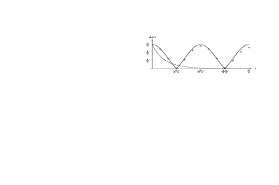
Figure 3: The quantum and classical probability distributions as functions of time $t$. The solid line corresponds to $\Delta^{Q}\left(t\right)$, and the dashed line to $\Delta^{C}\left(t\right)$, both in theory. The crosses corresponds to the experimental results of the quantum case.

III Experimental Implementation

For the quantum CTRW on a circle with four node, the Hilbert space is 4-demensional. So it is natural to implement the quantum walks on a two-qubit quantum computer. The direct correspondence is to map the basis {$\left|0\right\rangle$, $\left|1\right\rangle$, $\left|2\right\rangle$, $\left|3\right\rangle\}$ of the quantum CTRW into the four computational basis {$\left|0\right\rangle\otimes\left|0\right\rangle$, $\left|0\right\rangle\otimes\left|1\right\rangle$, $\left|1\right\rangle\otimes\left|0\right\rangle$, $\left|1\right\rangle\otimes\left|1\right\rangle$}. This mapping is in fact to rephrase the number of nodes by the binary number system. Therefore the Hamiltonian in equation (1) can be written as

$$H=2\gamma I\otimes I-\gamma\left(I\otimes\sigma_{x}+\sigma_{x}\otimes\sigma_{x}\right),$$ (9)

where $I$ and $\sigma_{x}$ are the identity operator and the Pauli operator of a single qubit. The evolution operator of the two-qubit system is

$$U\left(t\right) =e^{-iHt}$$

$$=e^{-2i\gamma t}\exp\left[i\gamma t\left(\sigma_{x}\otimes\sigma_{x}\right)\right]\exp\left[i\gamma t\left(I\otimes\sigma_{x}\right)\right].$$ (10)

And the state of a particle performing this quantum CTRW is

$$\left|\psi\left(t\right)\right\rangle =e^{-2i\gamma t}\cos^{2}\gamma t\left|00\right\rangle-e^{-2i\gamma t}\sin{}^{2}\gamma t\left|10\right\rangle$$

$$+\frac{i}{2}e^{-2i\gamma t}\sin 2\gamma t\left(\left|01\right\rangle+\left|11\right\rangle\right).$$ (11)

It is interesting to investigate the relations between the distribution of the implemented quantum CTRW and the entanglement of the two-qubit state $\left|\psi\left(t\right)\right\rangle$. The entanglement of the two-qubit state $\left|\psi\left(t\right)\right\rangle$ in equation (11) can be directly calculated by the Von. Neumann entropy

$$S\left(t\right)=-\cos^{2}\gamma t\log_{2}\left(\cos^{2}\gamma t\right)-\sin{}^{2}\gamma t\log_{2}\left(\sin^{2}\gamma t\right).$$ (12)

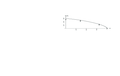
Figure 4: The correlation between the quantum total variation distance $\Delta^{Q}\left(t\right)$ and the entanglement $S\left(t\right)$. The line corresponds to theoretical calculation. The experimental results in different sets are shown in different shapes. The triangles are for $n\in\left\{1,2,3\right\}$, crosses for $n\in\left\{4,5,6\right\}$, boxes for $n\in\left\{7,8,9\right\}$ and circles for $n\in\left\{10,11,12\right\}$.

The correlation between the quantum total variation distance $\Delta^{Q}\left(t\right)$ and the entanglement $S\left(t\right)$ is illustrated in FIG. 4. From FIG. 4, we can see that if there is no entanglement between the two qubits ($S=0$), $\Delta^{Q}$ is at its maximal $\Delta^{Q}=\frac{3}{4}$, which corresponds converging at node $0$ (or node $2$). While if the two qubits are maximally entangled ($S=1$), $\Delta^{Q}=0$, which happens to be the situation that the walking particle is uniformly distributed on the four nodes. Therefore, we can say that the quantum random walk algorithm is enhanced by the quantum entanglement involved.

The quantum CTRW is implemented using our two-qubit NMR quantum computer. This computer uses a $0.5$ milliliter, $200$ millimolar sample of Carbon-13 labeled chloroform (Cambridge Isotopes) in d${}_{\text{6}}$ acetone. In a magnetic field, the two spin states of ${}^{\text{1}}$H and ${}^{\text{13}}$C nuclei in the molecular can be described as four nodes of two qubits, while radio frequency (RF) fields and spin–spin couple constant $J$ are used to implement quantum network of CTRW. Experimentally, we performe twelve separate sets of experiments with various selection of time $t$ which is distinguished by $\gamma t=\frac{n\cdot\pi}{12}\left(n=\left\{0,1,2,\cdots,12\right\}\right)$. In the following, we replace the jumping rate $\gamma$ with $\pi J$ $(J=215Hz)$. In each set, the full process of the quantum CTRW is executed. We describe this experimental process as follows.

Firstly, prepare effective pure state $\left|\psi\left(0\right)\right\rangle$: The initial state in NMR is thermally equilibrium state $\rho_{eq}\equiv 4I_{z}^{1}+I_{z}^{2}$ rather than a true pure state $\left|\psi\left(0\right)\right\rangle$. However, it is possible to create an effective pure state, which behaves in an equivalent manner. This is implemented as

$$R_{x}^{1}\left(\pi/3\right)-G_{z}-R_{x}^{1}\left(\pi/4\right)-\tau-R_{y}^{1}\left(-\pi/4\right)-G_{z},$$

to be read from left to right, radio-frequency pulses are indicated by $R_{axis}^{spins}\left(angle\right)$, and are applied to the spins in the superscript, along the axis in the subscript, by the angle in the brackets. For example, $R_{x}^{1}\left(\pi/3\right)$ denotes $\pi/3$ selective pulse that acts on the first qubit about $\widehat{x}$, and so forth. $G_{z}$ is the pulsed field gradient along the $\widehat{z}$ axis to annihilate transverse magnetizations, dashes are for readability only, and $\tau$ represents a time interval of $1/\left(2J\right)$. Therefore, after the state preparation, we obatin effective pure state $\rho\left(0\right)\equiv I_{z}^{1}+I_{z}^{2}+2I_{z}^{1}I_{z}^{2}$ from equilibrium state $\rho_{eq}\equiv 4I_{z}^{1}+I_{z}^{2}$.

Secondly, perform quantum CTRW with different time $t$: As shown above in equation (10), quantum CTRW can be described as unitary operator $U\left(t\right)$, this is performed with pulse sequence shown in the following (Note that the global phase $e^{-2i\gamma t}$ of $U\left(t\right)$ is safely ignored in our experiments, since $\rho\left(t\right)=U\left(t\right)\rho\left(0\right)U\left(t\right)^{{\dagger}}$, this global phase is meaningless and has no effect on the result of experiment)

$$R_{x}^{2}\left(\theta\right)-R_{y}^{12}\left(\pi/2\right)-\frac{t}{2}-R_{x}^{12}\left(\pi\right)-\frac{t}{2}-R_{y}^{12}\left(-\pi/2\right).$$

Here $R_{x}^{2}\left(\theta\right)$ is equal to $e^{-i\frac{\theta}{2}\widehat{\sigma}_{x}}$ that act on the second spin,where $\theta=n\pi/6$ and $t=n/\left(6J\right)=n\pi/\left(6\gamma\right)$ for $n\in\left\{1,2,\cdots,12\right\}$, $R_{x}^{12}\left(\pi\right)$ denotes $\pi$ non-selective pulse that acts on both qubits about $\widehat{x}$. It is obviously that the final state $\rho\left(t\right)$ of the quantum CTRW prior to measure is given by $\rho\left(t\right)=U\left(t\right)\rho\left(0\right)U\left(t\right)^{{\dagger}}$.

Finally, readout the result $\rho\left(t\right)$ and calculate quantum total variation distance $\Delta^{Q}\left(t\right)$: In NMR experiment, it is not practical to determine the final state directly, but an equivalent measurement can be made by so-called quantum state tomography to recover the density matrix $\rho\left(t\right)=\left|\psi\left(t\right)\right\rangle\left\langle\psi\left(t\right)\right|$. However, as only the diagonal elements of the final density operators are needed in our experiments, the readout procedure is simplified by applying gradient pulse before readout pulse to cancel the off-diagonal elements. Here we shall note that, the gradient pulse can remove off-diagonal terms since we use heteronuclear systems in our experiment. Then quantum total variation distance $\Delta^{Q}\left(t\right)$ is determined by the equation $\Delta^{Q}\left(t\right)=\tfrac{1}{2}{\textstyle\sum\nolimits_{k=0}^{3}}\left|P_{k}^{Q}\left(t\right)-\tfrac{1}{4}\right|$, where $P_{k}^{Q}\left(t\right)=\left\langle k\right|\rho\left(t\right)\left|k\right\rangle\$ is certain probability on the node $\left|k\right\rangle$. Finally, $\Delta^{Q}\left(S\right)$ is determined with equation (12).

All experiments are conducted at room temperature and pressure on Bruker Avance DMX-500 spectrometer in Laboratory of Structure Biology, University of Science and Technology of China. FIG. 3 show the quantum total variation distance $\Delta^{Q}\left(t\right)$ as a function of time $t$ and FIG. 4 show the quantum total variation distance $\Delta^{Q}\left(S\right)$ as a function of entanglement $S$ of $\left|\psi\left(t\right)\right\rangle$ shown in equation (11). From FIG. 3 and FIG. 4, it is clearly seen the good agreement between theory and experiment. However, there exist small errors which increase when time $t$ increase, we think that the most errors are primarily due to decoherence, because the time used to implement quantum CTRW $U\left(t\right)$ is increased from several to several tens milliseconds approximately, while the decoherence time $T_{2}\approx 0.3$ and $0.4$ seconds for carbon and proton respectively. The other errors are due to inhomogeneity of magnetic field, imperfect pulses, and the variability over time of the measurement process.

IV Conclusion

We present the experimental implementation of the quantum random walk algorithm on a two-qubit nuclear magnetic resonance quantum computer. For the quantum CTRW on a circle with four nodes, we observe that the quantum walk behaves greatly differently from its classical version. The quantum CTRW can yield an exactly uniform distribution, and is reversible and periodic, while the classical walk is essentially dissipative. Further, we find that the property of this quantum walk strongly depends on the quantum entanglement between the two qubits. The uniform distribution could be obtained only when the two qubits are maximally entangled. In this paper only the relatively simple case with two qubits are considered. However, our scheme could be extended to the case of a graph containing arbitrary $N$ nodes, and the quantum random walk could be carried out by using $\log_{2}N$ qubits.

- (1) P.W. Shor, in Proceedings of the 35th Annual Symposium on Foundations of Computer Science (IEEE Computer Society Press, Los Alamitos, CA, 1994), p. 124.
- (2) L.K. Grover, Phys. Rev. Lett. 79, 325 (1997).
- (3) N.A. Nielsen and I.L. Chuang, Quantum Computation and Quantum Information (Cambridge University Press, Cambridge, 2000).
- (4) R.P. Feynman, Int. J. Theor. Phys. 21, 467 (1982).
- (5) Y. Aharonov, et al., Phys. Rev. A 48, 1687 (1993).
- (6) E. Farhi and S. Gutmann, Phys. Rev. A 58, 915 (1998).
- (7) A. Ambainis, et al., in Proceedings of the 30th annual ACM Symposium on Theory of Computing (Association for Computing Machinery, New York, 2001).
- (8) A.M. Childs et al., quant-ph/0103020; C. Moore and A. Russell, quant-ph/0104037; N. Konno et al., quant-ph/0205065; J. Kempe, quant-ph/0205083; T. Yamasaki et al., quant-ph/0205045; E. Bach et al., quant-ph/0207008.
- (9) B.C. Travaglione and G.J. Milburn, Phys. Rev. A 65, 032310 (2002).
- (10) W. Dür et al., Phys. Rev. A 66, 052319 (2002).
- (11) M.N. Barber and B.W. Ninham, Random and Restricted Walks: Theory and Applications (Gordon and Breach, New York, 1970).
- (12) A.M. Childs et al., quant-ph/0209131; N. Shenvi et al., quant-ph/0210064.
- (13) J.I. Cirac and P. Zoller, Phys. Rev. Lett. 74, 4091 (1995).
- (14) C. Monroe et al., Phys. Rev. Lett. 75, 4714 (1995).
- (15) D.G. Cory, A.F. Fahmy, and T.F. Havel, Proc. Natl. Acad. Sci. USA 94, 1634 (1997); N. Gershenfeld and I. Chuang, Science 275, 350 (1997).
- (16) M.A. Nielsen, E. Knill and R. Laflamme, Nature 396, 52 (1998).
- (17) D.G. Cory et al., Phys. Rev. Lett. 81, 2152 (1998); D. Leung et al., Phys. Rev. A 60, 1924 (1999); E. Knill et al., Phys. Rev. Lett. 86, 5811 (2001).
- (18) S. Somaroo et al., Phys. Rev. Lett. 82, 5381 (1998).
- (19) L.M.K. Vandersypen et al., Nature 414, 883 (2002); I.L. Chuang et al., Nature 393, 143 (1998); J.A. Jones, M. Mosca and R.H. Hansen, Nature 393, 344 (1998); R. Marx et al., Phys. Rev. A 62, 012310 (2000); J. Du et al., Phys. Rev. A 64, 042306 (2001). L.Xiao et al., Phys. Rev. A 66, 052320 (2002). X. Peng et al., Phys. Rev. A 65, 042315 (2002). J. Zhang et al., Phys. Rev. A 66, 044308 (2002).
- (20) J. Du et al., Phys. Rev. Lett. 88, 137902 (2002).
- (21) X. Fang et al., Phys. Rev. A 61, 022307 (2000); J. Du et al., Phys. Rev. A 63, 042302 (2001); D. Collins et al., Phys. Rev. A 62, 022304 (2000).