Generation of polarization-entangled photon pairs in a cascade of
two type-I crystals pumped by femtosecond pulses

Abstract

We report the generation of polarization-entangled photons by femtosecond-pulse-pumped spontaneous parametric down-conversion in a cascade of two type-I crystals. Highly entangled pulsed states were obtained by introducing a temporal delay between the two orthogonal polarization components of the pump field. They exhibited high-visibility quantum interference and a large concurrence value, without the need of post-selection using narrow-bandwidth-spectral filters. The results are well explained by the theory which incorporates the space-time dependence of interfering two-photon amplitudes if dispersion and birefringence in the crystals are appropriately taken into account. Such a pulsed entangled photon well localized in time domain is useful for various quantum communication experiments, such as quantum cryptography and quantum teleportation.

]

I INTRODUCTION

Photon pairs generated in the process of spontaneous parametric down-conversion (SPDC) have been an effective and convenient source of two-particle entangled states used in tests on the foundations of quantum mechanics as well as application to quantum information technologies such as quantum cryptography and quantum teleportation. In such applications, a pulsed source of entangled photon pairs is particularly useful because the times of emission are known to the users. For example, in the entanglement-based quantum key distribution protocol[1, 2, 3], it is convenient to share entangled photons between sender and receiver in a train of short optical pulses synchronized with the common timing clock pulses. Such a pulsed source allows the sender and receiver to know the arrival times of the photons within the duration of the pump pulse and to time stamp each received bit readily so that they can sift their raw data to generate a shared key from their public discussion. A pulsed source is also crucial in a certain class of experiments that require the use of several photon pairs at a time, such as quantum teleportation[4, 5, 6], entanglement distillation[7], and the generation of multiphoton entangled states[8, 9, 10]. In these experiments, time-synchronized entangled photon pairs must be available. It has also been pointed out that primitive elements of a quantum computer can be constructed from the combined use of several entangled photons and Bell-state measurement[11, 12].

A great deal of effort has been devoted to developing a pulsed source of entangled photon pairs. Over the past decade, femtosecond-pulse-pumped SPDC has been extensively studied by several groups. It has been shown that the entangled states generated in type-II SPDC pumped by ultrashort pulses shows disappointingly low visibility of the quantum interference, and narrow- bandwidth filters are required to increase the visibility at the expense of the photon flux[13, 14, 15]. Theoretical studies revealed that the down-converted photons are entangled simultaneously in polarization and space-time, or equivalently, wave number-frequency because of the significant effects of dispersion and birefringence in the crystal[13, 16, 17]. As a result of this multiple-entanglement, it is possible to distinguish, with some degree of certainty, which of the interfering pathways occurs by the measurement that distinguishes the space-time component of the state, for example, the measurement of the arrival time of the photons at the detector. This distinguishing space-time information is enough to seriously degrade the visibility of two-photon polarization interference. The presence of this distinguishing space-time information stems from the fact that the down-converted photons are emitted spontaneously, but the times of emission are known to be within the duration of the pump pulse. The resultant two-photon state is well localized in space-time, and provide undesirable timing capability. The situation is serious in the ultrashort-pulse-pumped SPDC, but is absent in the ordinary cw-pumped SPDC. Therefore, it is vital in the ultrashort-pulse-pumped SPDC to ensure that the space-time component of the state contained no distinguishing “which-path” information for the photons in order to observe the entanglement and quantum interference in the polarization degree of freedom. Various interferometric techniques have been proposed to eliminate the entanglement in unnecessary degrees of freedom and to recover the quantum interference[17, 18, 19, 20, 21].

On the other hand, cw-pumped SPDC exhibits a polarization-entanglement with high-visibility quantum interference capability. In particular, Kwiat et al. realized maximally polarization-entangled photons using noncollinear SPDC with type-II phase matching[22]. More recently, they demonstrated that noncollinear SPDC using two spatially separate type-I nonlinear crystals pumped by a cw laser exhibits high-visibility quantum interference[23]. The latter source is particularly convenient since the desired polarization-entangled states are produced directly out of the nonlinear crystal with unprecedented brightness and stability and without the need for critical optical alignment. Their result attracted great attention for the experimentalists. Recently, Kim et al. showed that polarization-entangled photons from two spatially separated type-I nonlinear crystals pumped by femtosecond laser pulses exhibit high-visibility interference[18]. In their experiment, collinear degenerate type-I SPDC and a beam splitter were used to create a polarization-entangled state. The state prepared after the beam splitter was, however, not considered to be entangled without amplitude postselection. Only when one considers those postselected events (half of the total events) in which photons traveled to different output ports, one can observe quantum interference. Later, this problem was solved by using collinear nondegenerate type-I SPDC and a dichroic beam splitter[19]. It was shown that mostly maximally entangled states showing high-visibility (92%) quantum interference were obtained without amplitude and spectral postselection just before detection. However, the available flux of the entangled photon pairs was still very limited ($\leq$100 s^-1).

In this paper, we apply femtosecond-pulse pumping to the second Kwiat scheme with type-I phase-matching arrangement. We shall demonstrate that highly entangled polarization states with sufficiently large flux are obtained when an appropriate temporal compensation is given in the pump pulses. The results will be shown to be consistent with the theory which incorporates the space-time dependence of interfering two-photon amplitudes, if the effects of dispersion and birefringence in the two-crystals are appropriately taken into account.

II EXPERIMENT

Our experimental setup is schematically shown in Fig. 1. Two adjacent, thin, type-I crystals (BBO) whose optic axes are horizontally (H) and vertically (V) oriented, respectively, are pumped by 45^∘- polarized femtosecond pulses at 266 nm. The pump pulses were third harmonic of a mode-locked output of Ti/Sapphire laser, whose approximate average power was 150 mW and repetition rate was 82 MHz. Due to type-I coupling, H-polarized photon pairs at 532 nm are generated by the V-polarization component of the pump field in the first crystals, and V-polarized photon pairs are generated by the H-polarization component of the pump field in the second crystal. These two possible down-conversion processes equally likely occurs and are coherent with one another[24, 25]. The SPDC was performed under a degenerate and quasi-collinear condition. The signal and idler photons making an angle of 3^∘ with respect to the pump laser beam and having the same wavelength around 532 nm were observed through the identical interference filters, centered at 532 nm, placed in front of the detectors. The polarization correlations were measured using polarization analyzers, each consisting of a rotatable half- wave plate (HWP) and a quarter-wave plate (QWP) (for 532 nm) followed by a polarizing beam splitter (PBS). After passing through adjustable irises, the photons were collected using 60-mm-focal-length lenses, and directed onto the detectors. The detectors (PMT) were photomultipliers (HAMAMATSU H7421-40) placed at $\sim$1.5 m from the crystal, with efficiencies of $\sim$40% at 532 nm and dark count rates of the order of 80 s^-1. The photodetection area was about 5 mm in diameter. The outputs of the detectors were recorded using a time interval analyzer (YOKOGAWA TA-520), and pulse pairs received within a time window of 7 ns were counted as coincident.

To obtain a truly polarization-entangled state, care must be taken to disentangle the polarization degree of freedom from any other degrees of freedom, that is, to factorize the total state into product of the polarization- entangled state and those describing other degrees of freedom. This is equivalent to saying that effective polarization entanglement requires the suppression of any distinguishing information in the other degrees of freedom that can provide potential information about “which-polarization” the emitted pair have. In our case, since which crystal the origin of each pair is and their polarization are intrinsically correlated, distinguishing “which-crystal” information must be also eliminated. Accordingly, to make emitted spatial modes for a given pair indistinguishable for the two crystals, we overlap the down-conversion light cones spatially by using very thin crystals each having $\sim$130 $\mu$m-thickness. In addition, it is important to eliminate distinguishing space-time information inherent in the two-photon states produced in the ultrashort-pulse-pumped SPDC. Figure 2 schematically illustrates what may happen when a 45^∘- polarized femtosecond pulse incidents on two cascaded type-I BBO crystals, which is estimated roughly from the optical characteristics of the BBO[26]. For simplicity, we consider here the degenerate collinear SPDC. In the first crystal, H-polarized down-converted photon wavepackets are advanced at $\sim$74 fs relative to the V-polarized pump pulse due to group velocity dispersion, while the H-polarized pump pulse is delayed at $\sim$61 fs relative to the V-polarized pump pulse due to birefringence in the BBO. In the second crystal, V-polarized down-converted photon wavepackets are advanced at $\sim$74 fs relative to the H-polarized pump pulse due to group velocity dispersion, while the H-polarized down-converted photon wavepackets are advanced at $\sim$242 fs relative to the H-polarized pump pulse due to an advance given in the first crystal ($\sim$135 fs) and dispersion in the second crystal ($\sim$107 fs). Consequently, after the crystals, space-time components of the two-photon state associated with the polarization states $\left|HH\right\rangle$ and $\left|VV\right\rangle$ are expected to be temporally displaced by $\sim$168 fs, where $\left|H\right\rangle$ ($\left|V\right\rangle$) means a single photon linearly polarized along a horizontal (vertical) axis and the first (second) letter corresponds to the signal (idler). Note that the distance between the two BBO crystals is not an important factor in this consideration. Since down-converted photon wavepackets are expected to have widths comparable to that of pump field ($\sim$150 fs), it is suggested that the space-time components associated with $\left|HH\right\rangle$ and $\left|VV\right\rangle$ do not overlap in space-time. As a result, “which-polarization” information may be available, in principle, from the arrival time of the photons at the detector.

To eliminate this distinguishing space-time information, a polarization dependent optical delay line for the 266-nm pump was inserted before the crystals, which is denoted as the pre-compensator in Fig. 1. It consists of quartz plates, whose optic axes are oriented either vertically or horizontally, and a Bereck-type tiltable polarization compensator. The combination of the quartz plates of various thicknesses provides a relative delay of $\left|T\right|\leq$350 fs between the H- and V-polarization components of the 266-nm pump field, while the sign is given by the orientation of its optic axis. This delay line can compensate for relative delay between the state associated with $\left|HH\right\rangle$ created in the first crystal relative to the state associated with $\left|VV\right\rangle$ created in the second crystal to overlap them temporally. The Bereck-type polarization compensator is used to adjust the subwavelength delay. As a result, a two-photon Bell state $\left|\Phi^{+}\right\rangle=(\left|HH\right\rangle+\left|VV\right\rangle)/\sqrt{2}$ can be directly created.

Two kinds of experiments were carried out to confirm whether the target state $\left|\Phi^{+}\right\rangle$ was successfully prepared. The first experiment was a quantum state tomography[27]. The polarization density matrices were estimated from 16 kinds of joint projection measurements performed on an ensemble of identically prepared photon pairs. These joint measurements consist of four kinds of projection measurements onto {$\left|H\right\rangle,\left|V\right\rangle,\left|D\right\rangle,\left|L\right\rangle$} on each member of a photon pair, where $\left|D\right\rangle=(\left|H\right\rangle+\left|V\right\rangle)/\sqrt{2}$ and $\left|L\right\rangle=(\left|H\right\rangle+i\left|V\right\rangle)/\sqrt{2}$. We used a maximum likelihood calculation[28] to estimate the density matrix. We also calculated the concurrence of the state, which is known to give a good measure for the entanglement of a two-qubit system[29]. The second experiment was a conventional two-photon polarization interference experiment. In this experiment, QWPs in mode 1 and mode 2 were set to 0^∘, i.e., their optic axes were vertically oriented, while HWP in mode 1 was set to $\pm$22.5^∘ and HWP in mode 2 was rotated. In our setup, this corresponds to the projection measurements onto {$\left|L\right\rangle$ or $\left|R\right\rangle$}$\otimes\left|\theta\right\rangle$, where $\left|R\right\rangle=(\left|H\right\rangle-i\left|V\right\rangle)/\sqrt{2}$ and $\left|\theta\right\rangle=\cos 2\theta\left|H\right\rangle+i\sin 2\theta\left|V\right\rangle$. The visibility of an observed interference pattern gives another convenient measure for the entanglement.

At first, we used the interference filters having a full-width half maximum (FWHM) bandwidth of 8 nm in front of the detectors. Figure 3 illustrates the estimated polarization density matrices prepared when (a) no relative delay, (b) relative delay of 135 fs, and (c) relative delay of 231 fs were introduced between the H- and V-polarization components of a 266-nm pump field. In these experiments, maximum coincidence counts and typical accidental coincidence counts were $\sim$450 cps and $<$10 cps, respectively. As shown by these examples, we could successfully prepare the states approximately described by $\rho(v)=\frac{1-v}{2}(\left|HH\right\rangle\left\langle HH\right|+\left|VV\right\rangle\left\langle VV\right|)+v\left|\Phi^{+}\right\rangle\left\langle\Phi^{+}\right|$. These states should exhibit interference in coincidence rates for the two detectors in proportion to $P(\theta)=\frac{1}{4}(1\pm v\sin 4\theta)$. Figure 4 shows the coincidence rates as a function of the HWP angle in mode 2 and the evaluated visibilities associated with the states in Fig. 3(a)-(c). Note that, no background was subtracted in these results, so that the evaluated visibilities give the lower limits of $v$. The experiments were repeated for various values of delay $T$ introduced in the H- and V-polarization components of the pump field. The evaluated concurrence C and visibility v of the polarization interference are plotted in Fig. 5 as a function of relative delay $T$. This figure clearly indicates that there is a strong correlation between the concurrence and the visibility. This is quite natural because $C=v$ should hold for the states $\rho(v)$ given by the above form. In this experiment, the maximum values of the concurrence and visibility were 0.95 and 0.92$\pm$0.02, respectively. The broken line in Fig. 5 is a Gaussian curve fitted to the measured data, and the FWHM width is 237 fs.

Next, to investigate the effects of interference filters used in front of the detectors, we replaced them with those having a FWHM bandwidth of 40 nm. Figure 6 shows C and v evaluated by the same procedure, except that the backgrounds have been subtracted for both the concurrence and the visibility data in this case. The maximum values of C and v were slightly reduced to 0.92 and 0.90, respectively, while the maximum coincidence counts were increased by a factor of $\approx$ 6. (Unfortunately, the accidental coincidence increased more than six times, which is probably due to ambient light.) The broken line in Fig. 6 is a Gaussian curve fitted to the measured data, and the FWHM width is $\approx$205 fs. The width of the fitted curve was slightly reduced in comparison with that for the 8-nm filters, which was due to the spectral filtering effects, as shown later.

We also measured the autocorrelation of the pump field by measuring the degree of polarization, or equivalently, the magnitude of the Stokes parameter $\left|{\bf s}\right|=\sqrt{s_{1}^{2}+s_{2}^{2}+s_{3}^{2}}$ of the pump just after the pre-compensator (and before the crystals), where $s_{1}$, $s_{2}$, and $s_{3}$ are three independent Stokes parameters. Simple analysis shows that $\left|{\bf s}\right|$ is proportional to the temporal overlap of the H- and V- polarization components of the pump field between which relative delay $T$ was introduced by the pre-compensator, and directly gives the autocorrelation of the pump field. Figure 7 shows the measured $\left|{\bf s}\right|$ as a function of $T$. We found that $\left|{\bf s}\right|$ can be fitted with a Gaussian curve having a FWHM width $\approx$216 fs. Assuming the transform limited Gaussian-shape pulse, the FWHM temporal width of the pump field is estimated to be $\approx$153 fs, and that of the pump intensity to be $\approx$108 fs. We see that the width of the autocorrelation of the pump field is comparable to that of the measured concurrence and visibility data shown in Figs. 5 and 6. This result suggests that the width of the measured concurrence and visibility data are determined chiefly by the temporal width of the pump field.

III THEORETICAL ANALYSIS

Experimental results are analyzed based on the theory given by Grice et al.[14], Keller et al.[16], and Kim et al.[17]. In the following analysis, we will focus our attention on the Gaussian curve fitted with the measured concurrence and visibility data shown in Figs. 5 and 6, which will be denoted by $V(T)$. In particular, we will analyze how the widths of these curves are determined and depend on the experimental parameters. To make the following discussion self-contained, it may be helpful to begin by showing the minimum of the previous theories before discussing our problem. Let us consider the degenerate, quasi-collinear SPDC in a single type-I crystal pumped by a field with the central frequency $\Omega_{p}$ and the FWHM temporal width $\tau_{p}^{FWHM}$. For simplicity we ignore the transverse components of the photon wave vector. Let $\omega_{p}[\omega_{s},\omega_{i}]$ be the frequency and $k_{p}(\omega_{p})[k_{s}(\omega_{s}),k_{i}(\omega_{i})]$ the wave number for the pump [signal, idler]. The perfect phase-matching condition is given by $\Omega_{s}=\Omega_{i}=\Omega_{p}/2$ for the frequency and $K_{o}(\Omega_{s})+K_{o}(\Omega_{i})=K_{e}(\Omega_{p})$ for the wave number, where $K_{j}(\Omega)$ denotes the wave number for a photon having a frequency $\Omega$ and polarization along the ordinary (j=o) or extraordinary (j=e) optic axis. To simplify the notation, we introduce detuning for the signal, the idler, and the pump from the perfect phase-matching condition by $\nu_{s}=$ $\omega_{s}-\Omega_{p}/2$, $\nu_{i}=$ $\omega_{i}-\Omega_{p}/2$, and $\nu_{p}=\omega_{p}-\Omega_{p}$, respectively. To first-order in the interaction, the general expression of the two-photon state after the crystal is[14]

$$\left|\Psi\right\rangle=\frac{1}{2\pi}\int\int d\nu_{s}d\nu_{i}\Psi(\nu_{s},\nu_{i})a^{\dagger}(\nu_{s})b^{\dagger}(\nu_{i})\left|0\right\rangle,$$ (1)

where $a^{\dagger}(\nu_{s})$ and $b^{\dagger}(\nu_{i})$ are the photon creation operators for the o-polarized signal and idler modes characterized by detuning frequencies $\nu_{s}$ and $\nu_{i}$, respectively, which are defined after the crystal. The function $\Psi(\nu_{s},\nu_{i})$ is the two-photon amplitude in the frequency domain, and is given by [14]

$$\Psi(\nu_{s},\nu_{i})=\left\langle 0\right|a(\nu_{s})b(\nu_{i})\left|\Psi\right\rangle=C\alpha(\nu_{s}+\nu_{i})\Theta(\nu_{s},\nu_{i}).$$ (2)

In this expression, $\alpha(\nu_{p})$ is the spectral envelop function of the time-dependent classical pump field at the input surface of the crystals, $\Theta(\nu_{s},\nu_{i})$ is the longitudinal phase-matching function[14], and C is a constant. Assuming a Gaussian shape for the temporal envelop function of the pump field, $\alpha(\nu_{p})$ is given by

$$\alpha(\nu_{p})=e^{-\left(\frac{\nu_{p}}{\sigma_{p}}\right)^{2}},$$ (3)

where $\sigma_{p}=\sigma_{p}^{FWHM}/2\sqrt{\ln 2}$ $=4\sqrt{\ln 2}/\tau_{p}^{FWHM}$ is the FWHM bandwidth of the pump field. If z-direction is taken to be the pump direction, the longitudinal phase-matching function $\Theta(\nu_{s},\nu_{i})$ is given by

$$\Theta(\nu_{s},\nu_{i})=\frac{1}{L}\int_{-L/2}^{L/2}dze^{-i\Delta(\nu_{s},\nu_{i})z}=\mathop{\rm sinc}[\frac{\Delta(\nu_{s},\nu_{i})}{2}L],$$ (4)

where L is the crystal length, $\Delta(\nu_{s},\nu_{i})=k_{s}(\nu_{s}+\Omega_{p}/2)+k_{i}(\nu_{i}+\Omega_{p}/2)-k_{p}(\nu_{p}+\Omega_{p})$ is the phase mismatch and approximately given by[16, 17]

$$\Delta(\nu_{s},\nu_{i})=D_{+}\left(\nu_{s}+\nu_{i}\right)+\frac{1}{4}D^{\prime\prime}\left(\nu_{s}-\nu_{i}.\right)^{2}.$$ (5)

In this expression, $D_{+}$ and $D^{\prime\prime}$ are crystal parameters: $D_{+}\equiv 1/u_{o}(\Omega_{p}/2)-1/u_{e}(\Omega_{p})$ is the group velocity mismatch where $u_{o}(\Omega_{p}/2)$ ($u_{e}(\Omega_{p})$) is the group velocity of the o-polarized down-converted photons (the e-polarized pump photon) inside the crystal and $D^{\prime\prime}\equiv d^{2}K_{o}/d\Omega^{2}|_{\Omega=\Omega_{p}/2}$ is the group velocity dispersion for the down-converted photons.

Since we are interested in the temporal characteristics of the down-converted photons, we next consider the two-photon state after the crystal in the time domain. Formally, it can be written as

$$\left|\Psi\right\rangle=\int\int dt_{s}dt_{i}\hat{\Psi}(t_{s},t_{i})a^{\dagger}(t_{s})b^{\dagger}(t_{i})\left|0\right\rangle,$$ (6)

where $a^{\dagger}(t_{s})$ and $b^{\dagger}(t_{i})$ are Fourier transforms of $a^{\dagger}(\nu_{s})$ and $b^{\dagger}(\nu_{i})$. For example,

$$a^{\dagger}(t_{s})=\frac{1}{\sqrt{2\pi}}\int d\nu_{s}e^{i\left(\nu_{s}+\Omega_{p}/2\right)(t_{s}-L_{s}/c)}a^{\dagger}(\nu_{s}),$$ (7)

where $L_{s}$ is the optical path length from the output face of the crystal to the observation point. Physically, $t_{s}$ and $t_{i}$ are interpreted as the time of arrival of the idler and signal at the points that are $L_{s}$ and $L_{i}$ away from the output face of the crystal[30], and $\hat{\Psi}(t_{s},t_{i})$ gives information about the space-time motion of the two-photon wavepackets. The two-photon amplitude in the time domain is simply given by the Fourier transform of the two-photon amplitude in the frequency domain and by[30]

$$\hat{\Psi}(t_{s},t_{i}) = \left\langle 0\right|a(t_{s})b(t_{i})\left|\Psi\right\rangle$$ (8)

$$= \frac{e^{-i\Omega_{p}t_{s}}}{2\pi}\int\int d\nu_{s}d\nu_{i}e^{-i(\nu_{s}t_{s}+\nu_{i}t_{i})}\Psi(\nu_{s},\nu_{i}).$$ (9)

We can further change the variables according to $\nu_{+}=$ $\nu_{s}+\nu_{i}=\nu_{p}$, $\nu_{-}=\nu_{s}-\nu_{i}$, $t_{+}=(t_{s}+t_{i})/2$, and $t_{-}=(t_{s}-t_{i})/2$, and obtain the equivalent Fourier transform relation

$$\hat{\psi}(t_{+},t_{-}) = \frac{e^{-i\Omega_{p}t_{s}}}{2\pi}$$ (11)

$$\times\int\int d\nu_{+}d\nu_{-}e^{-i(\nu_{+}t_{+}+\nu_{-}t_{-})}\psi(\nu_{+},\nu_{-}),$$

where $\psi(\nu_{+},\nu_{-})=\Psi(\frac{\nu_{+}+\nu_{-}}{2},\frac{\nu_{+}-\nu_{-}}{2})$ and $\hat{\psi}(t_{+},t_{-})=\hat{\Psi}(t_{+}+t_{-},t_{+}-t_{-})$. Physically, $t_{-}$ and $t_{+}$ mean half the difference in the arrival time, and the mean arrival time of the idler and signal photons, at the points that are $L_{s}$ and $L_{i}$ away from the output face of the crystal, respectively. The absolute square of the two-photon amplitude $\left|\hat{\psi}(t_{+},t_{-})\right|^{2}$ is proportional to the probability of arrival of the idler and signal at the given points for the given mean arrival time $t_{+}$ and half the difference in the arrival time $t_{-}$. We show schematically the relevant amplitudes in the time domain and the frequency domain in Fig. 8.

Now, let us proceed to provide a phenomenological model that is consistent with our experiment using two crystals. We assume down-conversion processes are equally likely to occur in two crystals whose optic axes are orthogonally oriented and thy are coherent with one another. We represent the overall two-photon state after the crystals as a superposition of the states arising from the SPDC in each crystal with appropriate phase. Then the two-photon state after the crystals in the time domain can be written as

$$\left|\Psi\right\rangle = \frac{1}{\sqrt{2}}\int\int dt_{+}dt_{-}$$ (14)

$$\times\{\hat{\psi}_{HH}(t_{+},t_{-})a_{H}^{\dagger}(t_{+}+t_{-})b_{H}^{\dagger}(t_{+}-t_{-})$$

$$+e^{i\phi}\hat{\psi}_{VV}(t_{+},t_{-})a_{V}^{\dagger}(t_{+}+t_{-})b_{V}^{\dagger}(t_{+}-t_{-})\}\left|0\right\rangle$$

$$= \frac{1}{\sqrt{2}}\int\int dt_{+}dt_{-}$$ (17)

$$\times\{\hat{\psi}_{HH}(t_{+},t_{-})\left|H,t_{+}+t_{-}\right\rangle_{s}\left|H,t_{+}-t_{-}\right\rangle_{i}$$

$$+e^{i\phi}\hat{\psi}_{VV}(t_{+},t_{-})\left|V,t_{+}+t_{-}\right\rangle_{s}\left|V,t_{+}-t_{-}\right\rangle_{i}\}$$

where the first (second) term represents the two-photon state generated in the first (second) crystal, and $\phi$ is the phase difference between the states generated in the two crystals. In Eq. 17 we incorporated a new dichotomic variable in the creation operators and the two-photon amplitudes that specifies the polarization (H or V) of the photon, and wrote $\left|H,t_{+}+t_{-}\right\rangle_{s}=a_{H}^{\dagger}(t_{+}+t_{-})\left|0\right\rangle$ etc., which denotes a single-photon state for the signal (or idler) mode characterized by a definite polarization and time. From the previous discussion, two two-photon amplitudes $\hat{\psi}_{HH}(t_{+},t_{-})$ and $\hat{\psi}_{VV}(t_{+},t_{-})$ are expected to be temporally displaced by $\tau$ in the $t_{+}$-direction due to dispersion and birefrengence in the crystals. On the other hand, the pre-compensator for the pump before the crystals introduces temporal displacement in the $t_{+}$-direction for these amplitudes by $-T_{p}$. Therefore, we postulate that these two amplitudes can be written using a single common amplitude as $\hat{\psi}_{HH}(t_{+},t_{-})=\hat{\psi}_{VV}(t_{+}+T,t_{-})\equiv\hat{\psi}(t_{+}+T,t_{-})$, where $T=\tau-T_{p}$. In this case, the two-photon state is now entangled both in polarization and in space-time, in other words, it is doubly entangled. The space-time components $\hat{\psi}_{HH}(t_{+},t_{-})$ and $\hat{\psi}_{VV}(t_{+},t_{-})$ provide the distinguishing information for the interfering path of the two-photon amplitudes and degrade polarization entanglement. The full density matrix associated with the state given in Eq. 17 can be written as

$$\rho_{ijkl}(t_{1},t_{2},t_{3},t_{4})=_{i}\left\langle j,t_{2}\right|_{s}\left\langle i,t_{1}|\Psi\right\rangle\left\langle\Psi|k,t_{3}\right\rangle_{s}\left|l,t_{4}\right\rangle_{i},$$ (18)

where $i,j,k,l=H$ or $V$. Since our chief concern is the polarization state of the photon pair, we will calculate the effective density matrix of the two-photon state after the two crystals that are defined in the polarization space alone. It can be calculated by partially tracing the density matrix in Eq. 18 over the time-variable, and is given by

$$\rho_{ijkl}=\int\int dt_{1}dt_{2}\rho_{ijkl}(t_{1},t_{2},t_{1},t_{2}).$$ (19)

Explicit calculation gives the effective density matrices of the form

$$\rho = \frac{1}{2}(\left|HH\right\rangle\left\langle HH\right|+\left|VV\right\rangle\left\langle VV\right|$$ (21)

$$+v(T)e^{-i\phi}\left|HH\right\rangle\left\langle VV\right|+v^{\ast}(T)e^{i\phi}\left|VV\right\rangle\left\langle HH\right|),$$

where we used the normalization condition of the two-photon amplitude:

$$\int\int dt_{+}dt_{-}\left|\hat{\psi}_{jj}(t_{+},t_{-})\right|^{2}=1$$ (22)

and notation $\rho_{ijkl}=\left\langle ji\right|\rho\left|kl\right\rangle$ ($i,j,k,l=H$ or $V$). In Eq. 21, $v(T)$ is the convolution of the two-photon amplitudes in the time domain

$$v(T) = \int\int dt_{+}dt_{-}\hat{\psi}_{HH}(t_{+},t_{-})\hat{\psi}_{VV}^{\ast}(t_{+},t_{-})$$ (23)

$$= \int\int dt_{+}dt_{-}\hat{\psi}(t_{+}+T,t_{-})\hat{\psi}^{\ast}(t_{+},t_{-}).$$ (24)

It should be noted that $v(T)$ is, in general, a complex number. However, in the present experiment, we always make $v(T)e^{-i\phi}$ a real number $\left|v(T)\right|$ by using the Bereck-type polarization compensator. Then, the density matrix given in Eq. 21 is formally the same as what we observed in the experiment, and Eq. 24 indicates that their concurrence is determined by the convolution of the two-photon amplitudes in the time domain.

Based on the above theory, we have made several numerical calculations to elucidate the physics behind the measured $V(T)$ curves. We calculated two-photon amplitudes in the frequency and time domains using the experimental parameters: $D_{+}\approx-570$ fs/mm, $D^{\prime\prime}\approx 855$ fs²/mm, $L=0.13$ mm, and $\tau_{p}^{FWHM}=153$ fs[26]. Figure 9 shows (a) the (unnormalized) two-photon amplitude $\psi(\nu_{+},\nu_{-})$ and (b) $\hat{\psi}(t_{+},t_{-})$. We can see that the bandwidth of $\psi(\nu_{+},\nu_{-})$ is much wider in the $\nu_{-}$-direction than in the $\nu_{+}$-direction, while the temporal width of $\hat{\psi}(t_{+},t_{-})$ is much wider in the $t_{+}$-direction than in the $t_{-}$-direction. This is due to the Fourier-transform relations between $\psi(\nu_{+},\nu_{-})$ and $\hat{\psi}(t_{+},t_{-})$. We can also see that the temporal width of $\hat{\psi}(t_{+},t_{-})$ in the $t_{+}$-direction is $\approx\tau_{p}^{FWHM}$. Using these results, the magnitude of the convolution $\left|v(T)\right|$ is calculated and plotted in Fig. 10 together with the fitted curve of autocorrelation of the pump field shown in Fig. 7. We can see that $\left|v(T)\right|$ nearly agrees with the autocorrelation curve of the pump field. This indicates that the temporal shape of $\hat{\psi}(t_{+},t_{-})$ is approximately Gaussian in the $t_{+}$-direction and their widths are nearly equal to the temporal width of the pump field. This is consistent with the fact that, although there is a small difference in the width, the measured $V(T)$ curves nearly agree with the autocorrelation curve of the pump field as in Figs. 5-7.

Now, let us examine in more detail the origin of the different widths of the measured $V(T)$ curves in Figs. 5 and 6 in which the different bandwidth spectral filters were used. We will show that this was due to spectral filtering effects. So far, the two-photon amplitudes after the crystal and before the spectral filter have been discussed. They are intrinsic ones in the sense that they are determined only by the pump field and the crystal parameters and irrelevant to the spectral filters. In contrast, what we actually observed in the experiment was the two-photon state after the spectral filters. Hence, it is required to relate the state after the filters to the state before the filters to find the spectral filtering effects. This can be done straightforwardly. Suppose that the linear spectral filters used for the signal and idler have complex frequency responses expressed by $F_{s}(\nu_{s})$ and $F_{i}(\nu_{i})$, respectively. These functions are assumed to be normalized such that

$$\int d\nu_{s}\left|F_{s}(\nu_{s})\right|^{2}=\int d\nu_{i}\left|F_{i}(\nu_{i})\right|^{2}=1$$ (25)

holds. Then the two-photon amplitude after the filters are simply given by $\Psi_{F}(\nu_{s},\nu_{i})=\Psi(\nu_{s},\nu_{i})F_{s}(\nu_{s})F_{i}(\nu_{i})$. Since the two-photon amplitude in the time domain is related to that in the frequency domain by the Fourier-transform relations, the associated two-photon amplitude in the time domain is written as

$$\hat{\Psi}_{F}(t_{s},t_{i}) = \frac{e^{-i\Omega_{p}t_{s}}}{2\pi}\int\int d\nu_{s}d\nu_{i}e^{-i(\nu_{s}t_{s}+\nu_{i}t_{i})}\Psi_{F}(\nu_{s},\nu_{i})$$ (26)

$$= \frac{1}{\left(2\pi\right)^{2}}\int\int d\tau_{s}d\tau_{i}\hat{\Psi}(\tau_{s},\tau_{i})\hat{\Phi}(t_{s}-\tau_{s},t_{i}-\tau_{i}),$$ (27)

where $\hat{\Phi}(t_{s},t_{i})=\hat{F}_{s}(t_{s})\hat{F}_{i}(t_{i})$ is a normalized two-variable function that incorporates the temporal response of the filters, and $\hat{F}_{s}(t_{s})$ and $\hat{F}_{i}(t_{i})$ are the Fourier transform of $F_{s}(\nu_{s})$ and $F_{i}(\nu_{i})$, for example,

$$\hat{F}_{s}(t_{s})=\frac{1}{\sqrt{2\pi}}\int d\nu_{s}e^{i\left(\nu_{s}+\Omega_{p}/2\right)t_{s}}F_{s}(\nu_{s}).$$ (29)

Equation LABEL:eq17 indicates that the two-photon amplitude after the filters is given by the convolution of the two-photon amplitude before the filters $\hat{\Psi}(t_{s},t_{i})$ and the apparatus function for the filters $\hat{\Phi}(t_{s},t_{i})$. Because of this relation, the input function $\hat{\Psi}(t_{s},t_{i})$ is smoothed by the filter function $\hat{\Phi}(t_{s},t_{i})$ to yield broadened output function $\hat{\Psi}_{F}(t_{s},t_{i})$. It may be worth pointing out that Eq. LABEL:eq17 is formally analogous to the connection of phase-space probability distribution with the Wigner functions describing system and measuring apparatus (quantum ruler or filter)[31, 32]. In this case, the concurrence and visibility are determined by the convolution of the output function $\hat{\psi}_{F}(t_{+},t_{-})=\hat{\Psi}_{F}((t_{s}+t_{i})/2,(t_{s}-t_{i})/2)$ in contrast to Eq. 24, in which the input function $\hat{\psi}(t_{+},t_{-})$ appears. Accordingly, their widths depend on the temporal response of the filters, and equivalently, depend on the bandwidth of the filters. In general, the smaller the filter bandwidth is, the larger the width of the $V(T)$ curve is, and vice versa.

Now, let us discuss quantitatively the difference in the width of the measured $V(T)$ curves associated with the 8-nm and 40-nm filters. If we assume the frequency response functions $F_{s}(\nu_{s})$ and $F_{i}(\nu_{i})$ to be well approximated by the Gaussian function with FWHM widths $\Delta\nu$, the temporal widths of the associated response functions $\hat{F}_{s}(t_{s})$ and $\hat{F}_{i}(t_{i})$ is in proportion to $\Delta\nu^{-1}$. In our case, $\Delta t_{8nm}\approx 104$ fs for the 8-nm filter and $\Delta t_{40nm}\approx 20.8$ fs for the 40-nm filter. On the other hand, from the experimental results shown in Figs. 5 and 6, those consistent with the present theory are roughly estimated to be $\Delta t_{8nm}^{\prime}\approx 86.0$ fs and $\Delta t_{40nm}^{\prime}\approx 17.2$ fs. Here, we used the fact that the width $\sigma$ of the convolution of two Gaussian functions each having width $\sigma_{1}$ and $\sigma_{2}$ is given by $1/\sigma^{2}=1/\sigma_{1}^{2}+1/\sigma_{2}^{2}$. Therefore, even if there remain small quantitative discrepancies, it seems reasonable to conclude that there is considerable validity in the above simplified theory.

Let us switch our attention to the spectral characteristics. For the two-photon state given in Eq. 1, the joint spectral intensity is given by $I(\nu_{s},\nu_{i})\propto\left|\Psi(\nu_{s},\nu_{i})\right|^{2}$. Then the spectra $I_{s}(\nu_{s})$ and $I_{i}(\nu_{i})$ of the signal and the idler can be obtained by tracing $I(\nu_{s},\nu_{i})$ over the unobserved variable, for example,

$$I_{s}(\nu_{s})\propto\int d\nu_{i}I(\nu_{s},\nu_{i}).$$ (30)

Figure 11 shows the calculated individual spectra for the down-converted photons just after the crystal. This figure indicates that the FWHM bandwidth of the down-converted photons is $\approx 40$ nm. Thus, in our experiment using the 8-nm filters in front of the detectors, what we have observed is only a fraction of the photons having the wavelength $532\pm 4$ nm that can reach the detectors. On the contrary, we can safely say that almost all the photons produced in the SPDC have been observed in our experiment using the 40-nm filters. In other words, the coincidence count rate ($\approx 2700$ cps) obtained in the experiment using the 40-nm filters had already reached the upper limit in our configuration. However, since no optimization was made for the transversal spatial mode of the down-converted photons in this experiment, we believe that further improvement in the coincidence count rate may be possible by optimizing the experimental configuration[33, 34].

While our simplified model seems satisfactory in essence, there still remains a problem which needs to be solved. Within our model, the autocorrelation curve of the pump field should have the smallest width, whereas this is not the case. Although we have not arrived at a conclusion yet, there might be things neglected in this consideration that should actually have been taken into consideration. For example, we neglected the effect higher than the second-order optical nonlinearity in the crystal. There actually might occur higher order effects. In particular, it is likely that self-phase modulation (SPM) due to third-order optical nonlinearity occurs when the crystals are pumped by ultrashort optical pulses having large peak intensities. When the SPM is taken into account, the two-photon state after the crystal is chirped, and their coherence length might be shortened, and the resultant width of the measured $V(T)$ curves might be reduced. To obtain a more satisfactory explanation, the effect of SPM in the crystals might be incorporated into the theory.

IV CONCLUSION

In conclusion, we have generated pulsed polarization-entangled photon pairs by femtosecond-pulse-pumped SPDC in a cascade of two type-I crystals. It was found that highly entangled photon pairs were successfully obtained by using giving an appropriate temporal delay between the orthogonal polarization components for the pump, without the need of spectral post-selection using narrow-bandwidth filters. Theoretical analysis showed that entanglement depends on the convolution of the space-time components of the interfering two-photon amplitudes. The experimental results obtained were well explained if the dispersion and birefringence effects in the two-crystals are taken into account. Our analysis also revealed the effect of the spectral filtering on the magnitude of the entanglement when the interfering two-photon amplitudes has a different space-time dependence.

This work was supported by CREST of JST (Japan Science and Technology Corporation).

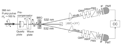
FIG. 1.: Experimental setup for generating and characterizing polarization entangled pulsed photons. The pump pulse polarized at 45^∘ irradiates a cascade of two type-I crystals, whose optic axes are orthogonally oriented. Pre-compensator (quartz plate and tiltable wave plate) introduces relative delays between the two-photon amplitudes created in the first and second crystal. CC is the coincidence circuit.

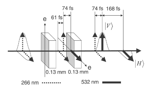
FIG. 2.: Schematic of the temporal development of the down-converted photons and the pump. See text for details.

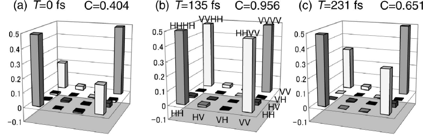
FIG. 3.: Estimated polarization density matrices for (a) no relative delay, (b) relative delay of 135 fs, and (c) relative delay of 231 fs between the H- and V-polarization components of the pump field. Only the real parts of the matrices are shown. The contribution of the imaginary parts is negligible. The dark-colored bars show diagonal elements, while the light-colored bars show off-diagonal elements. Estimated values of concurrence are shown as $C$.

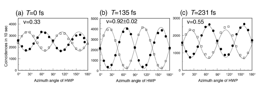
FIG. 4.: Polarization correlation experiment. Coincidence counts in 10 s is plotted against the orientation angle of the half-wave plate in mode 2, while the half-wave plate in mode 1 was fixed to $\pm 25.5{{}^{\circ}}$, for the states shown in (a)-(c) of Fig. 3. Estimated visibilities are also shown in the figure.

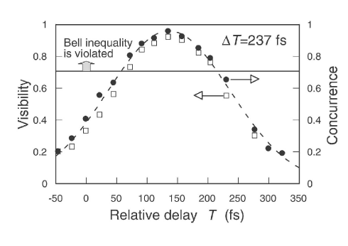
FIG. 5.: Evaluated concurrence C and visibility v when 8-nm interference filters were used. These values are plotted against the relative delay introduced between two orthogonal components of the pump field. The broken line is Gaussian fit to the data with 237-fs widths (FWHM).

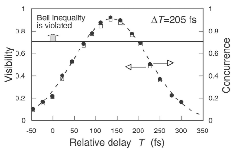
FIG. 6.: Evaluated concurrence C and visibility v when 40-nm interference filters were used. The broken line is Gaussian fit to the data with 205-fs widths (FWHM).

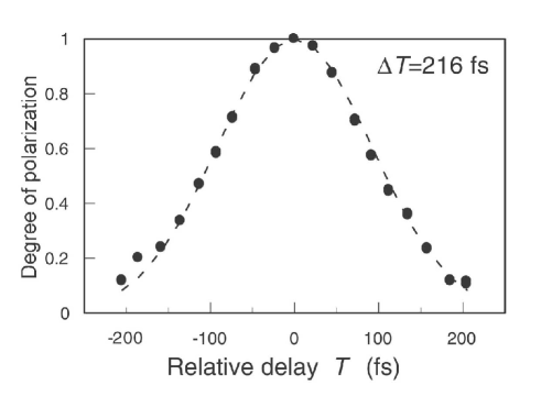
FIG. 7.: Autocorrelation of the pump field evaluated by measuring the degree of polarization after the pre-compensator. They are plotted against the relative delay introduced between two orthogonal components of the pump field. The broken line is Gaussian fit to the data with 216-fs widths (FWHM).

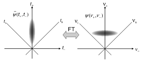
FIG. 8.: Illustration of two-photon amplitudes in the time and frequency domains generated by the femtosecond-pulse pump. For simplicity the case where $L_{s}=L_{i}=L$ is dipicted. They are connected by a Fourier transform relation.

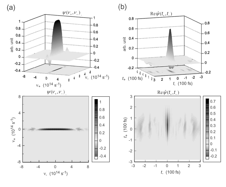
FIG. 9.: Calculated (unnormalized) two-photon amplitudes (a) in the frequency domain and (b) in the time domain. Only the real part of the amplitude is shown for the time domain. The contribution of the imaginary part is relatively lower.

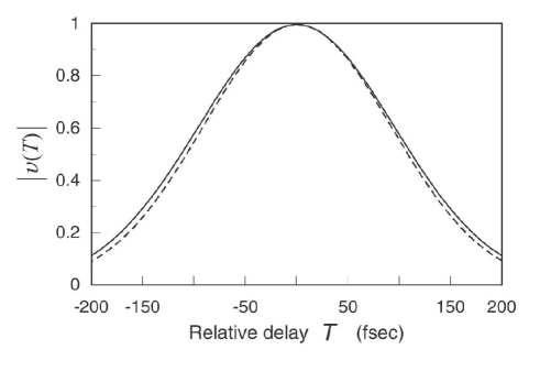
FIG. 10.: Calculated magnitude of the convolution $\left|v(T)\right|$. The broken line shows the autocorrelation of the pump field.

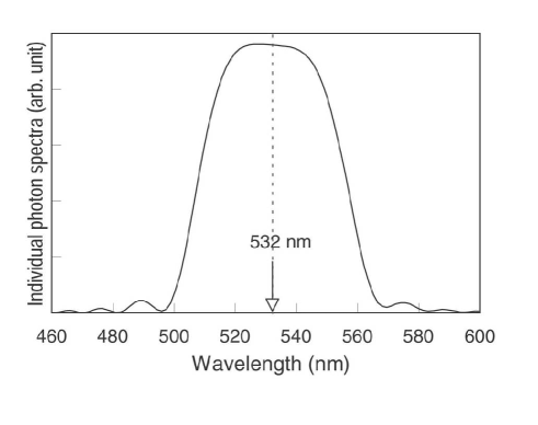
FIG. 11.: Calculated spectrum for the down-converted photons just after the crystal. Slight assymetry in the spectrum with respect to the phase-matching wavelength (=532 nm) is due to the combined effect of the group velocity mismatch and the group velocity dispersion in the nonlinear crystal.

REFERENCES

- [1] A. K. Ekert, G. M. Palma, J. G. Rarity, and P. R. Tapster, Phys. Rev. Lett. 69, 1923 (1992).
- [2] T. Jennewein, C. Simon, G. Weihs, H. Weinfuter, and A. Zeilinger, Phys. Rev. Lett. 84, 4729 (2000).
- [3] D. S. Naik, C. G. Peterson, A. G. White, A. J. Berglud, and P. G. Kwiat, Phys. Rev. Lett. 84, 4733 (2000).
- [4] C. H. Bennett, G. Brassard, C. Crépeau, R. Jozsa, A. Peres, and W. K. Wootters, Phys. Rev. Lett. 70, 1895 (1993).
- [5] D. Bouwmeester, J-W. Pan, K. Mattle, M. Eibl, H. Weinfuter, and A. Zeilinger, Nature (London) 390, 575 (1997).
- [6] D. Bouwmeester, K. Mattle, J-W. Pan, H. Weinfuter, A. Zeilinger, and M. Zukowski, Appl. Phys. B 67, 749 (1998).
- [7] C. H. Bennett, D. P. DiVincenzo, J. A. Smolin, and W. K. Wootters, Phys. Rev. A 54, 3824 (1996).
- [8] D. M. Greenberger, M. A. Horne, A. Shimony, and A. Zeilinger, Am. J. Phys. 58, 1131 (1990).
- [9] D. Bouwmeester, J-W. Pan, M. Daniell, H. Weinfuter, and A. Zeilinger, Phys. Rev. Lett. 82, 1345 (1999).
- [10] J-W. Pan, D. Bouwmeester, M. Daniell, H. Weinfuter, and A. Zeilinger, Nature 403, 515 (2000).
- [11] D. Gottesman and I. Chuang, Nature 402, 390 (1999).
- [12] D. Gottesman and I. Chuang, e-Archive quant-ph/9908010.
- [13] G. Di Guiseppe, L. Haiberger, F. De Martini, and A. V. Sergenko, Phys. Rev. A 56, R21 (1997).
- [14] W. P. Grice and I. A. Walmsky, Phys. Rev. A 56, 1627 (1997).
- [15] W. P. Grice, R. Erdmann, I. A. Walmsky, and D. Branning, Phys. Rev. A 57, R2289 (1998).
- [16] T. E. Keller and M. H. Rubin, Phys. Rev. A 56, 1534 (1997).
- [17] Y-H. Kim, M. V. Chekhova, S. P. Kulik, M. H. Rubin, and Y. Shih, Phys. Rev. A 63, 62301 (2001).
- [18] Y-H. Kim, S. P. Kulik, and Y. Shih, Phys. Rev. A 62, R011802 (2000).
- [19] Y-H. Kim, S. P. Kulik, and Y. Shih , Phys. Rev. A 63, 60301 (2001).
- [20] D. Branning, W. P. Grice, R. Erdmann, and I. A. Walmsky, Phys. Rev. Lett. 83, 955 (1999).
- [21] D. Branning, W. P. Grice, R. Erdmann, and I. A. Walmsky, Phys. Rev. A 62, 13814 (2000).
- [22] P. G. Kwiat et al., Phys. Rev. Lett. 75, 4337 (1995).
- [23] P. G. Kwiat et al., Phys. Rev. A 60, R773 (1999).
- [24] Z. Y. Ou, L. J. Wang, and L. Mandel, Phys. Rev. A 40, 1428 (1989).
- [25] Z. Y. Ou, L. J. Wang, X. Y. Zou, and L. Mandel, Phys. Rev. A 41, 566 (1990).
- [26] D. Eimerl, L. Davis, S. Velsko, E. K. Graham, and A. Zalkin, J. Appl. Phys. 62, 1968 (1987).
- [27] A. G. White, D. F. V. James, P. H. Eberhard, and P. G. Kwiat, Phys. Rev. Lett. 83, 3103 (1999).
- [28] D. F. V. James, P. G. Kwiat, W. J. Munro, and A. G. White, Phys. Rev. A 64, 52312 (2001).
- [29] W. K. Wootters, Phys. Rev. Lett. 80, 2245 (1998); Quantum Information and Computation, 1, 27 (2001).
- [30] M. H. Rubin, D. N. Klyshko, Y. H. Shin, and A. V. Sergienko, Phys. Rev. A 50, 5122 (1994).
- [31] K. Wódkiewicz, Phys. Rev. Lett. 52, 1064 (1984).
- [32] P. L. Knight, Quantum fluctuations in optical systems, in Quantum Fluctuations, Les Houches, Session LXIII, 1995, S. Reynaud, E. Giacobino, and J. Zinn-Justin eds. (Amsterdam, Elsevier 1997)
- [33] C. H. Kurtsiefer, M. Oberparleiter, and H. Weinfurter, e-Archive quant-ph/0101074.
- [34] C. H. Monken, P. H. S. Ribeiro, and S. Páuda, Phys. Rev. A 57, R2267 (1998).