Optimal parameter estimation of depolarizing channel

Abstract

We investigate strategies for estimating a depolarizing channel for a finite dimensional system. Our analysis addresses the double optimization problem of selecting the best input probe state and the measurement strategy that minimizes the Bayes cost of a quadratic function. In the qubit case, we derive the Bayes optimal strategy for any finite number of input probe particles when bipartite entanglement can be formed in the probe particles.

I Introduction

In order to design a reliable communication system one requires a priori knowledge of the property of a channel. Precise knowledge of the channel allows us to devise appropriate coding, modulation, and filtering schemes. In general, the channel property is not stationary, so one should first acquire and then track the optimal operating point of each device by monitoring the condition of the channel. It is important, therefore to know how to estimate the channel property in an efficient way, that is, as precisely as possible with minimum resources.

A reasonable assumption is that we know that the channel belongs to a certain parameterized family, and only the values of the parameters are not known. To know them one may input a probe system in an appropriate state into the channel and make a measurement on the output state. Only when an infinite amount of input resource is available, one can determine the channel parameters with perfect accuracy. In the quantum domain, however, the resource is often restricted for various reasons. For example, when one is to monitor a fast quantum dymanics at cryogenic temperatures, the input probe power should be kept as low as possible so as to prevent the system from heating up while obtaining meaningful data in a short time. This restricts the available amount of probe particles. Furthermore, preparing the probe in an appropriate quantum state is usually an elaborate process. Thus to find the efficient estimation strategy relying only on a restricted amount of input resource is of practical importance.

In estimating a quantum channel parameter, given a finite amount of input resource, both the input probe state and the measurement of the output state need to be optimized. This double maximization problem has been studied in the context of estimation of SU($d$) unitary operation  Acin01 . Estimating a noisy quantum channel has been discussed in the literature  Fujiwara01 ; Fischer01 ; Cirone01 . In ref. Fujiwara01 , the locally unbiased estimator and the Cramér-Rao bound are extensively discussed for the depolarizing channel for a qubit system. The locally optimal strategy, which achieves the Cramér-Rao bound at a local point of the parameter space was derived when two qubits at most are used. This result would be useful in the limit of large ensemble of the input probe. In such a limit, of course, one can establish the channel parameter with a very high degree of accuracy. To improve the rate at which the estimation accuracy grows with the number of probe particles, one may first apply some preliminary estimation using a part of probe particles to establish the most likely value of the parameter, and then use the locally optimal strategy around this value to get the final estimate  Barndorff98 ; Gill00 ; Hayashi02 . Refs. Fischer01 ; Cirone01 focus on several noisy qubit channels. They study some reasonable, although not optimal, strategies based on maximum likelyhood estimator, and derive the asymptotic behavior of the cost as a function of the number of input probe qubits.

In contrast, we are concerned here with the Bayes optimal strategy which minimizes the average cost. The scenario we have in mind is that one has no particular knowledge about the a priori parameter distribution, and the available number of probe particles is strictly limited. We then take into account the possibility of rather large errors. We seek the strategy that works equally well for all possible values of the parameter on average, that is, the strategy which is more universal for various possible situations.

It seems difficult for us to study this problem for the most general probe state. In this paper we deal with the depolarizing channel by assuming that we dispose of $M$ pairs of probe particles and only bipartite entanglement can be formed in each pair. This might be a practically sensible assumption from the view point of optical implementation given current technology. Our problem is to find the best estimation strategy to minimize the average cost. We consider the quadratic of a cost function.

II Qubit case

Let $\hat{\rho}$ be a density operator in the 2 dimensional Hilbert space ${\cal H}_{2}$. The depolarizing channel ${\cal L}_{\theta}$ maps a density operator $\hat{\rho}$ to a density operator which is a mixture of $\hat{\rho}$ and the maximally mixed state,

$${\cal L}_{\theta}\hat{\rho}=\theta\hat{\rho}+\frac{1-\theta}{2}\hat{I}.$$ (1)

The parameter $\theta$ represents the degree of randomization of polarization. For the map ${\cal L}_{\theta}$ to be completely positive, the parameter $\theta$ must lie in the interval $-{1\over 3}\leq\theta\leq 1$.

Let us start with two qubit systems as the input probe. For simplicity we only consider a pure state family of the probe $\hat{\Psi}=\left|\Psi\right\rangle\left\langle\Psi\right|$. This may be represented in the Schmidt decomposition

$$\left|\Psi\right\rangle=\sqrt{x}\left|0\right\rangle\otimes\left|e_{0}\right\rangle+\sqrt{1-x}\left|1\right\rangle\otimes\left|e_{1}\right\rangle,$$ (2)

where $\{\left|0\right\rangle,\left|1\right\rangle\}$ and $\{\left|e_{0}\right\rangle,\left|e_{1}\right\rangle\}$ are orthonormal basis sets for the first and second probe particle, respectively. What is the best way to use this state? There are two possibilities to consider;

• Input one qubit of the pair into the channel keeping the other untouched leading to the output state

  $$\hat{\Psi}_{1}(\theta)\equiv({\cal L}_{\theta}\otimes\hat{I})\left|\Psi\right\rangle\left\langle\Psi\right|,$$ (3)

• Input both qubits into the channel and have the output state

  $$\hat{\Psi}_{2}(\theta)\equiv({\cal L}_{\theta}\otimes{\cal L}_{\theta})\left|\Psi\right\rangle\left\langle\Psi\right|.$$ (4)

A measurement is described by a probability operator measure (POM) $\hat{\Pi}(\theta)$  Helstrom_QDET ; Holevo_book , also referred to as a positive operator valued measure (POVM) Peres_book . The average cost for the quadratic cost function is given by

$$\bar{C}_{i}(x)=\int_{-{1\over 3}}^{1}d\tilde{\theta}\int_{-{1\over 3}}^{1}d\theta(\tilde{\theta}-\theta)^{2}z(\theta)\mathrm{Tr}\left[\hat{\Pi}(\tilde{\theta})\hat{\Psi}_{i}(\theta)\right],$$ (5)

where $z(\theta)$ is the a priori probability distribution of $\theta$, and $\int_{-{1\over 3}}^{1}d\tilde{\theta}\hat{\Pi}(\tilde{\theta})=\hat{I}$. It is assumed that we have no a priori knowledge about $\theta$, that is, $z(\theta)={3\over 4}$. Given the channel ${\cal L}_{\theta}$, we are to find the optimal probe $\left|\Psi\right\rangle$ and the POM $\hat{\Pi}(\theta)$ minimizing the average cost $\bar{C}(x)$.

It is convenient to introduce the risk operator

$$\hat{W}(\theta) = {3\over 4}\int_{-{1\over 3}}^{1}d\theta^{\prime}(\theta-\theta^{\prime})^{2}\hat{\Psi}_{i}(\theta^{\prime}),$$ (6)

$$= \hat{W}^{(2)}-2\theta\hat{W}^{(1)}+\theta^{2}\hat{W}^{(0)},$$ (7)

where $\hat{W}^{(k)}\equiv{3\over 4}\int_{-{1\over 3}}^{1}d\theta\theta^{k}\hat{\Psi}_{i}(\theta)$. The average cost is then

$$\bar{C}(x)=\mathrm{Tr}\hat{\Gamma},\quad\hat{\Gamma}\equiv\int_{-{1\over 3}}^{1}d\theta\hat{\Pi}(\theta)\hat{W}(\theta).$$ (8)

For a fixed probe state $\left|\Psi\right\rangle$, the optimal POM $\hat{\Pi}(\theta)$ is derived from the necessary and sufficient conditions to minimize the average cost  Holevo73_condition ; YuenKennedyLax75 :

• $\hat{\Gamma}=\hat{\Gamma}^{\dagger}$, and $\left[\hat{W}(\theta)-\hat{\Gamma}\right]\hat{\Pi}(\theta)=0$ for all $\theta$,

• $\hat{W}(\theta)-\hat{\Gamma}\geq 0$ for all $\theta$.

The optimal solution for a single parameter estimation with a quadratic cost is well known  Personick71b ; Helstrom_QDET . The optimal POM is constructed by finding the eigenstate $\left|\theta\right\rangle$ of the minimizing operator $\hat{\Theta}$ which is defined by

$$\hat{\Theta}\hat{W}^{(0)}+\hat{W}^{(0)}\hat{\Theta}=2\hat{W}^{(1)},$$ (9)

that is, $\hat{\Pi}(\theta)=\left|\theta\right\rangle\left\langle\theta\right|$ so that $\hat{\Theta}\left|\theta\right\rangle=\theta\left|\theta\right\rangle$. We then have $\hat{\Gamma}=\hat{W}^{(2)}-\hat{\Theta}\hat{W}^{(0)}\hat{\Theta}$ from which the conditions (i) and (ii) are easily verified.

For a discrete system, one can find the optimal POM with finite elements. Let the spectral decomposition of $\hat{W}^{(0)}$ for our two-qubit system be

$$\hat{W}^{(0)}=\sum_{i=1}^{4}\omega_{i}\left|\omega_{i}\right\rangle\left\langle\omega_{i}\right|.$$ (10)

Then the minimizing operator is

$$\hat{\Theta}=\sum_{i,j=1}^{4}\frac{2}{\omega_{i}+\omega_{j}}\left|\omega_{i}\right\rangle\left\langle\omega_{i}\right|\hat{W}^{(1)}\left|\omega_{j}\right\rangle\left\langle\omega_{j}\right|.$$ (11)

Let the spectral decomposition of $\hat{\Theta}$ be

$$\hat{\Theta}=\sum_{i=1}^{4}\theta_{i}\left|\theta_{i}\right\rangle\left\langle\theta_{i}\right|.$$ (12)

The optimal POM is then given by

$$\hat{\Pi}(\theta)=\sum_{i=1}^{4}\delta(\theta-\theta_{i})\left|\theta_{i}\right\rangle\left\langle\theta_{i}\right|.$$ (13)

This implies that the measurement has 4 outputs at most and we then estimate the channel parameter as one of 4 $\theta_{i}$’s. Before going on to derive the optimal strategies, let us define some notations. As seen below the output states $\hat{\Psi}_{i}(\theta)$’s can be written as a direct sum

$$\hat{\Psi}_{i}(\theta)=\hat{\psi}_{i}(\theta)\oplus\hat{\phi}_{i}(\theta),$$ (14)

where $\hat{\psi}_{i}(\theta)$ is in the subspace $\cal{H}_{\psi}$ spanned by $\left|\mu_{1}\right\rangle\equiv\left|0\right\rangle\otimes\left|f_{0}\right\rangle$ and $\left|\mu_{2}\right\rangle\equiv\left|1\right\rangle\otimes\left|f_{1}\right\rangle$, and $\hat{\phi}_{i}(\theta)$ in the subspace $\cal{H}_{\phi}$ spanned by $\left|\nu_{1}\right\rangle\equiv\left|0\right\rangle\otimes\left|f_{1}\right\rangle$ and $\left|\nu_{2}\right\rangle\equiv\left|1\right\rangle\otimes\left|f_{0}\right\rangle$. In the following all 2$\times$2 matrices represent density operators in $\cal{H}_{\psi}$ with $\left|\mu_{1}\right\rangle=\left(\begin{array}[]{c}1\\ 0\end{array}\right)$ and $\left|\mu_{2}\right\rangle=\left(\begin{array}[]{c}0\\ 1\end{array}\right)$.

Case (a):

The output state $\hat{\Psi}_{1}(\theta)$ is given by

$$\hat{\psi}_{1}(\theta) = {1\over 2}\left[\begin{array}[]{cc}(1+\theta)x&2\theta\sqrt{x(1-x)}\\ 2\theta\sqrt{x(1-x)}&(1+\theta)(1-x)\end{array}\right],$$ (17)

$$\hat{\phi}_{1}(\theta) = \frac{1-\theta}{2}\Bigl{[}(1-x)\left|\nu_{1}\right\rangle\left\langle\nu_{1}\right|+x\left|\nu_{2}\right\rangle\left\langle\nu_{2}\right|\Bigr{]}.$$ (18)

The elements of the risk operator are

$$\hat{W}^{(0)} = {1\over 3}\Bigl{(}\left[\begin{array}[]{cc}2x&\sqrt{x(1-x)}\\ \sqrt{x(1-x)}&2(1-x)\end{array}\right]\oplus\hat{\varphi}_{1}\Bigr{)},$$ (21)

$$\hat{W}^{(1)} = {1\over{27}}\Bigl{(}\left[\begin{array}[]{cc}8x&7\sqrt{x(1-x)}\\ 7\sqrt{x(1-x)}&8(1-x)\end{array}\right]\oplus\hat{\varphi}_{1}\Bigr{)},$$ (24)

$$\hat{W}^{(2)} = {1\over{27}}\Bigl{(}\left[\begin{array}[]{cc}6x&5\sqrt{x(1-x)}\\ 5\sqrt{x(1-x)}&6(1-x)\end{array}\right]\oplus\hat{\varphi}_{1}\Bigr{)},$$ (27)

where $\hat{\varphi}_{1}=(1-x)\left|\nu_{1}\right\rangle\left\langle\nu_{1}\right|+x\left|\nu_{2}\right\rangle\left\langle\nu_{2}\right|$. After a lengthy but straightforward calculation (see Appendix A) we have

$$\hat{\Theta}={2\over 9}\left[\begin{array}[]{cc}1+x&2\sqrt{x(1-x)}\\ 2\sqrt{x(1-x)}&2-x\end{array}\right]\oplus{1\over 9}\hat{I}_{\phi}.$$ (28)

To diagonalize $\Theta$ we introduce $r=\sqrt{1+12x(1-x)}$ and

$$\mathrm{cos}\gamma=\sqrt{\frac{r-1+2x}{2r}},\quad\mathrm{sin}\gamma=\sqrt{\frac{r+1-2x}{2r}}.$$ (29)

The eigenstates and eigenvalues are then

$$\begin{array}[]{lll}\left|\theta_{1}\right\rangle&=\mathrm{cos}\gamma\left|\mu_{1}\right\rangle+\mathrm{sin}\gamma\left|\mu_{2}\right\rangle,&\theta_{1}=(3+r)/9,\\ \left|\theta_{2}\right\rangle&=-\mathrm{sin}\gamma\left|\mu_{1}\right\rangle+\mathrm{cos}\gamma\left|\mu_{2}\right\rangle,&\theta_{2}=(3-r)/9,\\ \left|\theta_{3}\right\rangle&=\left|\nu_{1}\right\rangle,&\theta_{3}=1/9,\\ \left|\theta_{4}\right\rangle&=\left|\nu_{2}\right\rangle,&\theta_{4}=1/9.\end{array}$$ (30)

The average cost finally reads

$$\bar{C}_{1}(x)=\mathrm{Tr}(\hat{W}^{(2)}-\Theta\hat{W}^{(0)}\Theta)={8\over{81}}\left[1+(x-{1\over 2})^{2}\right].$$ (31)

This is minimized by the maximally entangled state input

$$\left|\Psi\right\rangle=\frac{1}{\sqrt{2}}\left(\left|0\right\rangle\otimes\left|f_{0}\right\rangle+\left|1\right\rangle\otimes\left|f_{1}\right\rangle\right),$$ (32)

for which $\theta_{1}={5\over 9}$ and $\theta_{2}=\theta_{3}=\theta_{4}={1\over 9}$. Therefore the optimal measurement is actually constructed by the two projectors

$$\hat{\Pi}_{1}=\left|\Psi\right\rangle\left\langle\Psi\right|,\quad\hat{\Pi}_{2}=\hat{I}-\left|\Psi\right\rangle\left\langle\Psi\right|,$$ (33)

with the associated guesses $\theta_{1}={5\over 9}$ and $\theta_{2}={1\over 9}$, respectively. The minimum average cost is $\bar{C}_{1\mathrm{min}}={8\over 81}$.

Case (b):

The output state $\hat{\Psi}_{2}(\theta)=\hat{\psi}_{2}(\theta)\oplus\hat{\phi}_{2}(\theta)$ is given by

$$\hat{\psi}_{2}(\theta) = \left[\begin{array}[]{cc}{1\over 4}-({1\over 2}-x)\theta+\theta^{2}&\theta^{2}\sqrt{x(1-x)}\\ \theta^{2}\sqrt{x(1-x)}&{1\over 4}+({1\over 2}-x)\theta+\theta^{2}\end{array}\right],$$ (36)

$$\hat{\phi}_{2}(\theta) = \frac{1-\theta^{2}}{4}\hat{I}_{\phi}.$$ (37)

The elements of the risk operator are

$$\hat{W}^{(0)} = {1\over{27}}\left[\begin{array}[]{cc}4+9x&7\sqrt{x(1-x)}\\ 7\sqrt{x(1-x)}&13-9x\end{array}\right]$$ (40)

$$\oplus {5\over{27}}\hat{I}_{\phi},$$ (41)

$$\hat{W}^{(1)} = {1\over{27}}\left[\begin{array}[]{cc}7x&5\sqrt{x(1-x)}\\ 5\sqrt{x(1-x)}&7(1-x)\end{array}\right]$$ (44)

$$\oplus {1\over{27}}\hat{I}_{\phi},$$ (45)

$$\hat{W}^{(2)} = {1\over{405}}\left[\begin{array}[]{cc}4+75x&61\sqrt{x(1-x)}\\ 61\sqrt{x(1-x)}&79-75x\end{array}\right]$$ (48)

$$\oplus \frac{11}{405}\hat{I}_{\phi}.$$ (49)

The minimizing operator is (see Appendix LABEL:ap_b)

$$\hat{\Theta}=\frac{1}{17[13+8x(1-x)]}\left[\begin{array}[]{cc}a&c\\ c&b\end{array}\right]\oplus{1\over 5}\hat{I}_{\phi},$$ (50)

where

$$\begin{array}[]{lll}a&=&7x(35-20x+2x^{2}),\\ b&=&7x(17+16x+2x^{2}),\\ c&=&9[9-2x(1-x)]\sqrt{x(1-x)}.\end{array}$$ (51)

To diagonalize it we use $r=\sqrt{(a-b)^{2}+4c^{2}}$ and

$$\mathrm{cos}\gamma=\sqrt{\frac{r+a-b}{2r}},\quad\mathrm{sin}\gamma=\sqrt{\frac{r-a+b}{2r}}.$$ (52)

We then have the similar eigenstates to Eq. (30) and the eigenvalues $\theta_{1}=\theta_{+}$, $\theta_{2}=\theta_{-}$, and $\theta_{3}=\theta_{4}={1\over 5}$ with

$$\theta_{\pm}=\frac{119[1+2x(1-x)]\pm r}{34[13+8x(1-x)]}.$$ (53)

The average cost is then

$$\bar{C}_{2}(x)=\frac{8[391+606x(1-x)-10x^{2}(1-x)^{2}]}{2295[13+8x(1-x)]}.$$ (54)

This is an upward convex function, symmetric with respect to $x={1\over 2}$. The minimum is attained at $x=0,1$, that is, by separable input states. This reads $\bar{C}_{2\mathrm{min}}=\frac{184}{1755}$.

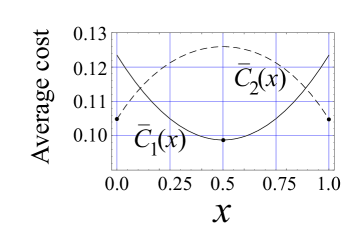
Figure 1: The average costs as a function of $x$.

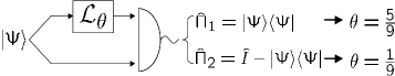
Figure 2: The optimal estimation strategy using two probe qubits. $\left|\Psi\right\rangle$ is the maximally entangled state. The output state is projected onto $\{\hat{\Pi}_{1},\hat{\Pi}_{2}\}$. We guess the channel parameter as $\theta={5\over 9}$ for the outcome $\hat{\Pi}_{1}$ and $\theta={1\over 9}$ otherwise.

The average costs for cases (a) and (b) are shown in Fig. 1: $\bar{C}_{1}(x)$ (solid line) and $\bar{C}_{2}(x)$ (dashed line). We see that $\bar{C}_{1\mathrm{min}}<\bar{C}_{2\mathrm{min}}$ so that the optimal estimation strategy, using two probe qubits, is to prepare them as a maximally entangled pair and to input one qubit of the pair into the channel keeping the other untouched. The estimation is then obtained by applying the two element POM, Eq. (33), as described in Case (a). This strategy is represented schematically in Fig. 2.

When $M$ maximally entangled pairs $\left|\Psi\right\rangle^{\otimes M}$ are available, it is best to use them so as to have the output $[({\cal L}_{\theta}\otimes\hat{I})\left|\Psi\right\rangle\left\langle\Psi\right|]^{\otimes M}$. The optimal measurement for this can be derived straightforwardly. This is discussed in the next section as a part of an arbitrary finite dimensional case.

III $d$-dimensional case

The action of the depolarizing channel on a $d$ dimensional system is described by

$${\cal L}_{\theta}\hat{\rho}=\theta\hat{\rho}+\frac{1-\theta}{d}\hat{I}.$$ (55)

Complete positivity then implies $-{1\over{d^{2}-1}}\leq\theta\leq 1$. For $d\geq 3$, we have not succeeded in finding the optimal probe state, even when we restrict ourselves to a pure state. In this section we focus on the most plausible input state, that is, the maximally entangled state, and consider the estimation using $M$ entangled pairs. Only for $d=2$, is the optimality ensured.

It might be interesting to compare the three cases specified by the three different outputs;

• $M$ product states of the pair

  $$\hat{\Psi}_{1}(\theta) = ({\cal L}_{\theta}\otimes\hat{I})\left|\Psi\right\rangle\left\langle\Psi\right|,$$ (56)

  $$= \theta\left|\Psi\right\rangle\left\langle\Psi\right|+\frac{1-\theta}{d^{2}}\hat{I}\otimes\hat{I},$$

  where $\left|\Psi\right\rangle$ is the maximally entangled state,

• $M$ product states of the pair

  $$\hat{\Psi}_{2}(\theta) = ({\cal L}_{\theta}\otimes{\cal L}_{\theta})\left|\Psi\right\rangle\left\langle\Psi\right|,$$ (57)

  $$= \theta^{2}\left|\Psi\right\rangle\left\langle\Psi\right|+\frac{1-\theta^{2}}{d^{2}}\hat{I}\otimes\hat{I},$$

• $2M$ product states of

  $$\hat{\psi}(\theta) = {\cal L}_{\theta}\left|0\right\rangle\left\langle 0\right|,$$ (58)

  $$= \theta\left|0\right\rangle\left\langle 0\right|+\frac{1-\theta}{d}\hat{I}.$$

(The input state in case (c) can be any pure state in the $d$ dimensional space.) Let us first consider the case (a). We denote Eq. (56) as

$$\hat{\Psi}(\theta)=f_{0}(\theta)\hat{a}_{0}+f_{1}(\theta)\hat{a}_{1},$$ (59)

where

$$\hat{a}_{0}\equiv\left|\Psi\right\rangle\left\langle\Psi\right|,\quad\hat{a}_{1}\equiv\hat{I}-\left|\Psi\right\rangle\left\langle\Psi\right|,$$ (60)

and

$$f_{0}(\theta)=\theta+\frac{1-\theta}{d^{2}},\quad f_{1}(\theta)=\frac{1-\theta}{d^{2}}.$$ (61)

The output state can then be represented as

$$\hat{\Psi}(\theta)^{\otimes M}=\sum_{m=0}^{M}f_{0}(\theta)^{M-m}f_{1}(\theta)^{m}\hat{A}_{m},$$ (62)

where

$$\hat{A}_{m}=\sum_{(i_{1}+...i_{M}=m)}\hat{a}_{i_{1}}\otimes\cdots\otimes\hat{a}_{i_{M}},$$ (63)

is the projector onto the symmetric subspace. The risk operator is

$$\hat{W}(\theta)=\sum_{m=0}^{M}[\omega_{m}^{(2)}-2\theta\omega_{m}^{(1)}+\theta^{2}\omega_{m}^{(0)}]\hat{A}_{m},$$ (64)

where $\omega_{m}^{(k)}\equiv\int_{-{1\over 3}}^{1}d\theta\theta^{k}f_{0}(\theta)^{M-m}f_{1}(\theta)^{m}$. The optimal POM is

$$\hat{\Pi}(\theta)=\sum_{m=0}^{M}\delta(\theta-\theta_{m})\hat{A}_{m},$$ (65)

where

$$\theta_{m}\equiv\frac{\omega_{m}^{(1)}}{\omega_{m}^{(0)}},$$ (66)

We then note that

$$\hat{W}(\theta)-\hat{\Gamma}=\sum_{m=0}^{M}(\theta-\theta_{m})^{2}\omega_{m}^{(0)}\hat{A}_{m}\geq 0,$$ (67)

from which it can easily be seen that the conditions (i) and (ii) hold. The minimum average cost is

$$\bar{C}_{1}(M)=\sum_{m=0}^{M}\left[\omega_{m}^{(2)}-\frac{(\omega_{m}^{(1)})^{2}}{\omega_{m}^{(0)}}\right]\left(\begin{array}[]{c}M\\ m\end{array}\right)(d^{2}-1)^{m}.$$ (68)

The other cases can be dealt with in a similar manner. In the case (b), we just put

$$f_{0}(\theta)=\theta^{2}+\frac{1-\theta^{2}}{d^{2}},\quad f_{1}(\theta)=\frac{1-\theta^{2}}{d^{2}}.$$ (69)

The minimum average cost $\bar{C}_{2}(M)$ is then given by the same expression as Eq. (68) with $\omega_{m}^{(k)}$’s defined by $f_{0}(\theta)$ and $f_{1}(\theta)$ of Eq. (69).

In the case (c), we use

$$\hat{a}_{0}\equiv\left|0\right\rangle\left\langle 0\right|,\quad\hat{a}_{1}\equiv\hat{I}-\left|0\right\rangle\left\langle 0\right|,$$ (70)

and

$$f_{0}(\theta)=\theta+\frac{1-\theta}{d},\quad f_{1}(\theta)=\frac{1-\theta}{d}.$$ (71)

The minimum average cost is

$$\bar{C}_{\mathrm{SEP}}(M)=\sum_{m=0}^{2M}\left[\omega_{m}^{(2)}-\frac{(\omega_{m}^{(1)})^{2}}{\omega_{m}^{(0)}}\right]\left(\begin{array}[]{c}2M\\ m\end{array}\right)(d-1)^{m}.$$ (72)

The three costs $\bar{C}_{1}(M)$, $\bar{C}_{2}(M)$, and $\bar{C}_{\mathrm{SEP}}(M)$ are plotted in Fig. 3 $(d=2)$, Fig. 4 $(d=3)$, and Fig. 5 $(d=10)$. In the figures another average cost $\bar{C}_{\mathrm{ML}}(M)$ is also plotted. This cost is by the strategy belonging to the case (c), but unlike the one attaining $\bar{C}_{\mathrm{SEP}}(M)$, the estimator is made by the maximum likelyhood principle for which

$$\theta_{m}=\frac{md}{2M(d-1)},$$ (73)

instead of Eq. (66), and leads to the analytic expression

$$\bar{C}_{\mathrm{ML}}(M)=\frac{1}{2M}\frac{d^{5}(d+3)}{6(d^{2}-1)^{3}}$$ (74)

It is this strategy that was used in ref. Cirone01 for the case of $d=2$.

For $d\geq 3$, the minimum average cost is always attained by a separable probe state. Only in the two dimensional case, is it the bipartite entangled probe that attains the minimum average cost. It is worth mentioning the depolarizing channel with the narrower parameter region $0\leq\theta\leq 1$, which is a more commonly used model with an well defined interpretation of randomized probability of $\theta$. We found that the best probe in this model is always a separable state. In this sense a separable state is generally an adequate probe state for the depolarizing channel estimation as far as the comparison with a bipartite entangled probe state is concerned.

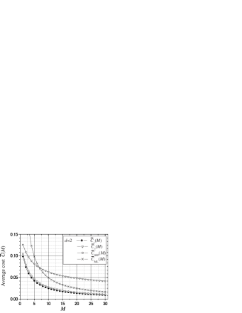
Figure 3: The average costs as a function of the number of pairs.

Figure 4: The average costs as a function of the number of pairs.

Figure 5: The average costs as a function of the number of pairs.

IV Concluding remark

When we have several identical samples at our disposal, it might be desirable to apply the best collective measurement on the whole system. This means preparing a single multi-qubit state followed by an optimized measurement. We might also consider performing a preliminary measurement on a part of the system and then feedback this back to deal with the remaining part. But in the case of the previous section, the collective measurement on $M$ identical output pairs or $2M$ identical output particles is not necessary. The action of the depolarizing channel on a maximally entangled state always results in a statistical mixture between the input state and its orthogonal complement (Eq. (59)). Estimating the channel parameter is nothing but determining this mixing ratio, which is a classical distribution. Therefore the optimal measurement is realized by a separable type constructed by the binary orthogonal projectors $\{\hat{a}_{0},\hat{a}_{1}\}$ according to Eq. (63). In the case where the output state includes the channel parameter as a quantum distribution, that is, the parameter appears in the off diagonal components in the density matrix, the optimal measurement would be a collective measurement. When the channel includes a unitary opreration, we will have to face this problem. Channel estimation for such a case is a future problem.

It is a remaining problem to see how effective the multipartite entangled probe is. However, in the estimation of decoherence channel under the power constraint scenario, that is, under a given and fixed number of probe particles, it seems more common that entanglement is not necessary. In fact, in the cases of the amplitude damping channel and dephasing channel, there is no merit to use entangled probe. In the amplitude damping channel, for example, the best probe is to input the most highly excited state. An entangled probe is rather wasteful because this includes the state components other than the excited state and these components are less sensitive to the damping.

Finally it might be interesting to study the multi parameter case, such as the Pauli channel estimation. We may then ask how to optimaize (in Bayesian sense) the simultaneous measurement on the noncommuting observables as well as searching for appropriate probe states.

*

Appendix A Derivation of Eq. (28)

For obtaining the minimizing operator $\Theta$ in Eq. (28), we first diagonalize $\hat{W}^{(0)}$ by $\hat{U}_{0}=\hat{u}_{0}\oplus\hat{I}_{\phi}$ where

$$\hat{u}_{0}=\left[\begin{array}[]{cc}\mathrm{cos}\gamma_{0}&-\mathrm{sin}\gamma_{0}\\ \mathrm{sin}\gamma_{0}&\mathrm{cos}\gamma_{0}\end{array}\right],$$ (75)

with $r_{0}=\sqrt{1-3x(1-x)}$ and

$$\mathrm{cos}\gamma_{0}=\sqrt{\frac{r_{0}-1+2x}{2r_{0}}},\quad\mathrm{sin}\gamma_{0}=\sqrt{\frac{r_{0}+1-2x}{2r_{0}}}.$$ (76)

The spectral decomposition

$$\hat{W}^{(0)}=\sum_{i=1}^{4}\omega_{i}\left|\omega_{i}\right\rangle\left\langle\omega_{i}\right|.$$ (77)

is given by

$$\begin{array}[]{lll}\left|\omega_{1}\right\rangle&=\hat{u}_{0}\left|\mu_{1}\right\rangle,&\omega_{1}=(1+r_{0})/3,\\ \left|\omega_{2}\right\rangle&=\hat{u}_{0}\left|\mu_{2}\right\rangle,&\omega_{2}=(1-r_{0})/3,\\ \left|\omega_{3}\right\rangle&=\left|\nu_{1}\right\rangle,&\omega_{3}=(1-x)/3,\\ \left|\omega_{4}\right\rangle&=\left|\nu_{2}\right\rangle,&\omega_{4}=x/3.\end{array}$$ (78)

We then calculate

$$\tilde{\Theta}=\sum_{i,j=1}^{4}\frac{2}{\omega_{i}+\omega_{j}}\left|i\right\rangle\left\langle\omega_{i}\right|\hat{W}^{(1)}\left|\omega_{j}\right\rangle\left\langle j\right|,$$ (79)

where

$$\begin{array}[]{lll}\left|1\right\rangle&=\left|\mu_{1}\right\rangle,\\ \left|2\right\rangle&=\left|\mu_{2}\right\rangle,\\ \left|3\right\rangle&=\left|\nu_{1}\right\rangle,\\ \left|4\right\rangle&=\left|\nu_{2}\right\rangle.\end{array}$$ (80)

This gives

$$\tilde{\Theta}=\tilde{\Theta}_{\psi}\oplus{1\over 9}\hat{I}_{\phi},$$ (81)

where

$$\tilde{\Theta}_{\psi}={1\over 9}\left[\begin{array}[]{cc}\frac{4r_{0}(1+r_{0})+3x(1-x)}{r_{0}(1+r_{0})}&-\frac{3(1-2x)\sqrt{x(1-x)}}{r_{0}}\\ -\frac{3(1-2x)\sqrt{x(1-x)}}{r_{0}}&\frac{4r_{0}(1-r_{0})-3x(1-x)}{r_{0}(1-r_{0})}\end{array}\right].$$ (82)

The minimizing operator is given by $\hat{\Theta}=\hat{U}_{0}\tilde{\Theta}\hat{U}_{0}^{\dagger}$ which results in Eq. (28).

Appendix B Derivation of Eq. (50)

The unitary operator for diagonalizing $\hat{W}^{(0)}$ in Eq. (41) is $\hat{U}_{0}=\hat{u}_{0}\oplus\hat{I}_{\phi}$ where

$$\hat{u}_{0}=\left[\begin{array}[]{cc}\mathrm{cos}\gamma_{0}&-\mathrm{sin}\gamma_{0}\\ \mathrm{sin}\gamma_{0}&\mathrm{cos}\gamma_{0}\end{array}\right],$$ (83)

with $r_{0}=\sqrt{81-128x(1-x)}$ and

$$\mathrm{cos}\gamma_{0}=\sqrt{\frac{r_{0}-9(1-2x)}{2r_{0}}},\quad\mathrm{sin}\gamma_{0}=\sqrt{\frac{r_{0}+9(1-2x)}{2r_{0}}}.$$ (84)

The spectral decomposition

$$\hat{W}^{(0)}=\sum_{i=1}^{4}\omega_{i}\left|\omega_{i}\right\rangle\left\langle\omega_{i}\right|.$$ (85)

is given by

$$\begin{array}[]{lll}\left|\omega_{1}\right\rangle&=\hat{u}_{0}\left|\mu_{1}\right\rangle,&\omega_{1}=(17+r_{0})/54,\\ \left|\omega_{2}\right\rangle&=\hat{u}_{0}\left|\mu_{2}\right\rangle,&\omega_{2}=(17-r_{0})/54,\\ \left|\omega_{3}\right\rangle&=\left|\nu_{1}\right\rangle,&\omega_{3}=5/27,\\ \left|\omega_{4}\right\rangle&=\left|\nu_{2}\right\rangle,&\omega_{4}=5/27.\end{array}$$ (86)

We then have

$$\tilde{\Theta}=\tilde{\Theta}_{\psi}\oplus{1\over 5}\hat{I}_{\phi},$$ (87)

where

$$\tilde{\Theta}_{\psi}=\left[\begin{array}[]{cc}\frac{7[r_{0}+9-16x(1-x)]}{r_{0}(17+r_{0})}&\frac{8(1-2x)\sqrt{x(1-x)}}{17r_{0}}\\ \frac{8(1-2x)\sqrt{x(1-x)}}{17r_{0}}&\frac{7[r_{0}-9+16x(1-x)]}{r_{0}(17-r_{0})}\end{array}\right].$$ (88)

Substituting this to $\hat{\Theta}=\hat{U}_{0}\tilde{\Theta}\hat{U}_{0}^{\dagger}$, we have Eq. (50).