Near-optimal two-mode spin squeezing via feedback

Abstract

We propose a feedback scheme for the production of two-mode spin squeezing. We determine a general expression for the optimal feedback, which is also applicable to the case of single-mode spin squeezing. The two-mode spin squeezed states obtained via this feedback are optimal for $j=1/2$ and are very close to optimal for $j>1/2$. In addition, the master equation suggests a Hamiltonian that would produce two-mode spin squeezing without feedback, and is analogous to the two-axis countertwisting Hamiltonian in the single-mode case.

I Introduction

Two-mode spin squeezed (TMSS) states are important to consider for a number of reasons. First, they may be used to demonstrate entanglement experimentally using only spin measurements Julsgaard . Second, as they are entangled, they may be used as a resource for quantum information, for example, quantum teleportation Kuzmich ; Berry , quantum computing, superdense coding, etc. NC . In addition, TMSS states are analogous to two-mode squeezed states for light Caves85 , which have proven to be useful for quantum information purposes Furusawa .

There are several approaches to produce TMSS states. Recently they have been produced experimentally for samples of atoms by quantum nondemolition (QND) measurements of the spin components Julsgaard . In Ref. Kuzmich it was proposed to produce TMSS states of light by combining the two Einstein-Podolsky-Rosen (EPR) output modes of an optical parametric oscillator with coherent light at polarizing beam splitters.

It is also possible to adapt proposals for generating single-mode spin squeezing to the two-mode case. For example, it has been proposed that single-mode spin squeezed states can be produced via an adiabatic approach Sor01 . In this approach, one starts with a Hamiltonian for which the ground state is easily achieved, and slowly varies the Hamiltonian towards one that has as its ground state the optimal spin squeezed state. In principle, this procedure can be adapted to obtain optimal TMSS states. A drawback to this method is that, in practice, the appropriate Hamiltonian may be difficult to realize.

Another technique for generating TMSS states that may be generalized from the single-mode case is feedback. Feedback has proven to be a powerful technique for state preparation Wise94 ; Laura and measurement Wise98 ; Berry01 . It has been shown that it is possible to produce near-optimal spin squeezing in the single-mode case by continual measurement of the spin operator $J_{z}$, and using feedback to bring $\langle{J_{z}}\rangle$ close to zero Laura . Here we adapt this method to the QND measurement approach discussed in Ref. Julsgaard .

The method for production of TMSS states in Ref. Julsgaard suffers the drawback that, although the variances in the sums of the spin components are small, their means are not close to zero. As is shown in Ref. Berry , the optimal TMSS states have zero means. We would therefore wish to obtain states with zero means in order for them to be as close as possible to the optimal states. This is analogous to the problem with the production of single-mode spin squeezing as considered by Thomsen, Mancini, and Wiseman (TMW) Laura .

II two-mode spin squeezing

In Ref. Julsgaard , TMSS states (conditioned on the measurement record) are obtained via QND measurements of the spin of the atomic samples. In order to perform this QND measurement, an off-resonant pulse is transmitted through two cesium gas samples. The interaction Hamiltonian may be expressed as Kuzmich ; KMJYEB

$$H_{\rm int}=\hbar a\int S_{z}(z,t)J_{z}(z,t)dz,$$ (1)

where $a$ is a coupling constant, $S_{z}(z,t)$ is the $z$ component of the instantaneous Stokes vector for the light, and $J_{z}(z,t)$ is the $z$ component of the continuous spin operator. These variables are explained further in Appendix A.

In the Schrödinger picture $J_{z}(z,t)$ is independent of $t$, and the total Stokes vector ${\bf S}(z)$ is independent of $z$. The total time evolution operator is, therefore,

$$U =\exp\left(-\frac{i}{\hbar}\int H_{\rm int}dt\right)$$

$$=\exp\left(-ia\int S_{z}(z,t)J_{z}(z)dz\,dt\right)$$

$$=\exp\left(-ia\int S_{z}J_{z}(z)dz\right)$$

$$=\exp(-iaS_{z}J_{z}).$$ (2)

In Ref. Julsgaard the light is initially linearly polarized, so the light is in the maximally weighted $S_{x}$ eigenstate. In addition, the total spin $s$ is large, so we may apply a SU(2)$\to$HW(2) contraction. That is, we make the substitutions Holstein ; Berry

$$S_{x} \to s-b^{\dagger}b,$$ (3)

$$S_{y} \to\sqrt{\frac{s}{2}}(b+b^{\dagger}),$$ (4)

$$S_{z} \to\frac{1}{i}\sqrt{\frac{s}{2}}(b-b^{\dagger}),$$ (5)

where $b^{\dagger}b$ is the number operator for photons subtracted from the $x$ linear polarization mode (and added to the $y$ linear polarization mode). We will assume that the probe beam is in a coherent spin state oriented in the $x$ direction (i.e., $x$ linearly polarized), and take the limit $s\to\infty$ so that this contraction is exact.

Under this contraction, $\left[S_{y},S_{z}\right]\to is$. This means that, under the Heisenberg picture, the operator $S_{y}$ transforms as

$$S_{y}^{\rm out}=S_{y}^{\rm in}+\left[iaS_{z}J_{z},S_{y}\right]\approx S_{y}^{\rm in}+\frac{an}{2}J_{z},$$ (6)

where $n=2s$ is the total number of photons in the pulse. Now we consider two samples, where we will use the notation $J_{k}^{(1)}$ and $J_{k}^{(2)}$, where $k\in\{x,y,z\}$, for the spin operators for samples 1 and 2, respectively, and $J_{k}^{(\pm)}=J_{k}^{(1)}\pm J_{k}^{(2)}$. We may replace $J_{z}$ with $J_{z}^{(+)}$, the total $z$ component of spin for the two samples, giving

$$S_{y}^{\rm out}\approx S_{y}^{\rm in}+\frac{an}{2}J_{z}^{(+)}.$$ (7)

Thus a measurement of $S_{y}^{\rm out}$ gives a QND measurement of $J_{z}^{(+)}$. In considering detection, it is more convenient to consider the Stokes vector for the light integrated over time interval $\delta t$. The transformation of this component is

$$\delta S_{y}^{\rm out}\approx\delta S_{y}^{\rm in}+\frac{a\delta n}{2}J_{z}^{(+)},$$ (8)

where $\delta n$ is the total number of photons in time $\delta t$. In Ref. Julsgaard , TMSS states are obtained by performing QND measurements on $J_{y}^{(+)}$ as well. They achieve this by applying a magnetic field in the $x$ direction, in order to induce Larmor precession of the $y$ and $z$ components of the spin. This means that Eq. (8) becomes

$$\delta S_{y}^{\rm out}(t)\approx\delta S_{y}^{\rm in}(t)+\frac{a\delta n}{2}[J_{z}^{(+)}\cos(\Omega t)+J_{y}^{(+)}\sin(\Omega t)],$$ (9)

where $\Omega$ is the frequency of the precession. In this case measurement of $\delta S_{y}^{\rm out}$ alternately gives QND measurements of $J_{z}^{(+)}$ and $J_{y}^{(+)}$, thus giving reduced uncertainty in both $J_{z}^{(+)}$ and $J_{y}^{(+)}$.

For the TMSS states considered in Ref. Julsgaard there is the requirement that $\langle{J_{x}^{(1)}}\rangle=-\langle{J_{x}^{(2)}}\rangle\gg 1$. Here we will instead take the convention that both $\langle{J_{x}^{(1)}}\rangle$ and $\langle{J_{x}^{(2)}}\rangle$ are large and close to the total spin $j$, and replace $J_{y}^{(+)}$ with $J_{y}^{(-)}$. This is equivalent to a trivial rotation of coordinates for one of the modes and does not require a physical alteration to the experiment. If we now define

$$J_{z}^{(\Omega)}(t)\equiv J_{z}^{(+)}\cos(\Omega t)+J_{y}^{(-)}\sin(\Omega t),$$ (10)

then Eq. (9) becomes

$$\delta S_{y}^{\rm out}(t)\approx\delta S_{y}^{\rm in}(t)+\frac{a\delta n}{2}J_{z}^{(\Omega)}(t).$$ (11)

In order for this to be accurate, we require $\delta n$ to be large, so that we may perform the SU(2)$\to$HW(2) contraction. Under this contraction, $\delta S_{y}=\sqrt{\delta s/2}X$, where $X=b+b^{\dagger}$. Therefore the transformation in the quadrature $X$ is

$$X^{\rm out}(t)=X^{\rm in}(t)+a\sqrt{\delta n}J_{z}^{(\Omega)}(t).$$ (12)

As the initial state is equivalent to the vacuum state [under the SU(2)$\to$HW(2) contraction], it has a variance of 1 in its measured value. The same is true for $X^{\rm out}$, as the extra term only changes the mean.

Measurements are made on the output beam by splitting the beam into $+45^{\circ}$ and $-45^{\circ}$ linearly polarized components at a polarizing beam splitter and measuring the intensities at the two outputs. We then define the photocurrent as

$$I_{c}(t)=\lim_{\delta t\to 0}\frac{\delta N_{+}-\delta N_{-}}{\sqrt{\nu}\delta t},$$ (13)

where $\delta N_{+}$ and $\delta N_{-}$ are the photon counts at the $+45^{\circ}$ and $-45^{\circ}$ linearly polarized outputs and $\nu$ is the photon flux $\delta n/\delta t$. We may interpret $I_{c}(t)$ as the measured value of $X$ divided by $\sqrt{\delta t}$, so the photocurrent is given by

$$I_{c}(t)=a\sqrt{\nu}\langle{J_{z}^{(\Omega)}}\rangle_{c}+\xi(t),$$ (14)

where the subscript $c$ indicates the average for the conditioned evolution, and $\xi(t)$ is a real Gaussian white noise term such that $\langle{\xi(t)\xi(t^{\prime})}\rangle=\delta(t-t^{\prime})$.

We take the limit of small time intervals $\delta t$, though for finite photon flux this would mean that the SU(2)$\to$HW(2) contraction is no longer valid, as $\delta n$ would go to zero. In order for the limit to be rigorously correct, we need to take the limit of large $\nu$ as well as small $\delta t$. Nevertheless, this limit should be an accurate approximation for large photon flux. The conditioned master equation is then

$$d\rho_{c}=\Gamma{\cal D}[J_{z}^{(\Omega)}]\rho_{c}dt+\sqrt{\Gamma}dW(t){\cal H}[J_{z}^{(\Omega)}]\rho_{c},$$ (15)

where $\Gamma=a^{2}\nu/4$, $dW(t)=\xi(t)dt$ is an infinitesimal Wiener increment, ${\cal D}[r]\rho=r\rho r^{\dagger}-(r^{\dagger}r\rho+\rho r^{\dagger}r)/2$, and ${\cal H}[r]\rho=r\rho+\rho r^{\dagger}-{\rm Tr}[(r+r^{\dagger})\rho]\rho$.

III Feedback

The quadrature (12) is measured by detecting the photocurrent (13), thereby yielding TMSS states. The drawback is that this will yield nonzero values of $\langle{J_{z}^{(+)}}\rangle$ and $\langle{J_{y}^{(-)}}\rangle$, whereas for the optimal TMSS states Berry , the expectation values are zero. In order to obtain states closer to the optimal TMSS states, we apply feedback to bring these expectation values closer to zero. For example, when $\cos(\Omega t)=1$, we may apply a Hamiltonian proportional to $J_{y}^{(+)}$ in order to bring $\langle{J_{z}^{(+)}}\rangle$ towards zero, analogous to the case considered by TMW. When $\sin(\Omega t)=1$, we wish to apply a Hamiltonian proportional to $J_{z}^{(-)}$ in order to bring $\langle{J_{y}^{(-)}}\rangle$ towards zero. For arbitrary $t$, we will apply the Hamiltonian

$$H_{\rm fb}=F(t)I_{c}(t),$$ (16)

where

$$F(t)=\frac{\lambda(t)}{\sqrt{\Gamma}}J_{y}^{(\Omega)}(t),$$ (17)

and

$$J_{y}^{(\Omega)}(t)\equiv J_{y}^{(+)}\cos(\Omega t)-J_{z}^{(-)}\sin(\Omega t).$$ (18)

We choose this definition for $J_{y}^{(\Omega)}$ because $[J_{z}^{(\Omega)},J_{y}^{(\Omega)}]=-iJ_{x}^{(+)}$ [we will omit the $(t)$ from this point for brevity]. As $\langle{J_{x}^{(+)}}\rangle$ is close to $2j$ for the states we are considering, this means that rotation about $J_{y}^{(\Omega)}$ will alter the expectation value of $J_{z}^{(\Omega)}$. This Hamiltonian may be implemented by a radio frequency magnetic field Sang . This generates a Hamiltonian proportional to $J_{y}$, which becomes $J_{y}^{(\Omega)}$ due to the Larmor precession of the atomic spin.

Using this feedback, we obtain the unconditioned master equation master

$$\dot{\rho}=-i[\tfrac{1}{2}\{c^{\dagger}F(t)+F(t)c\},\rho]+{\cal D}[c-iF(t)]\rho,$$ (19)

with

$$c=\sqrt{\Gamma}J_{z}^{(\Omega)}.$$ (20)

In the single-mode case TMW pointed out that the term $c^{\dagger}F(t)+F(t)c$ is proportional to $J_{z}J_{y}+J_{y}J_{z}$, which is the two-axis countertwisting Hamiltonian Kit . In a similar way we can derive a Hamiltonian for the two-mode case that produces TMSS states and is analogous to the two-axis countertwisting Hamiltonian. It is straightforward to show that

$$c^{\dagger}F(t)+F(t)c =\lambda(t)\{[(J_{y}^{(1)})^{2}+(J_{y}^{(2)})^{2}-(J_{z}^{(1)})^{2}$$

$$~{}-(J_{z}^{(2)})^{2}]\sin(2\Omega t)+(J_{z}^{(1)}J_{y}^{(1)}+J_{y}^{(1)}J_{z}^{(1)}$$

$$~{}~{}~{}+J_{z}^{(2)}J_{y}^{(2)}+J_{y}^{(2)}J_{z}^{(2)})\cos(2\Omega t)$$

$$~{}~{}~{}+2(J_{z}^{(1)}J_{y}^{(2)}+J_{y}^{(1)}J_{z}^{(2)})\}.$$ (21)

In the limit of large $\Omega$, the contribution to the evolution from the terms containing $\sin(2\Omega t)$ and $\cos(2\Omega t)$ is negligible. Omitting these terms yields

$$c^{\dagger}F(t)+F(t)c\approx 2\lambda(t)(J_{z}^{(1)}J_{y}^{(2)}+J_{y}^{(1)}J_{z}^{(2)}),$$ (22)

which indicates that it is possible to produce two-mode spin squeezing using the Hamiltonian

$$H\propto J_{z}^{(1)}J_{y}^{(2)}+J_{y}^{(1)}J_{z}^{(2)}.$$ (23)

III.1 Simple feedback

Now we will consider the appropriate feedback strength, $\lambda(t)$. It is easily shown that the variation in $\langle{J_{z}^{(\Omega)}}\rangle_{c}$ due to the conditioned evolution (15) is

$${\rm Tr}(J_{z}^{(\Omega)}d\rho_{c})=2\sqrt{\Gamma}dW[\langle{(J_{z}^{(\Omega)})^{2}}\rangle_{c}-\langle{J_{z}^{(\Omega)}}\rangle_{c}^{2}].$$ (24)

The variation in $\langle{J_{z}^{(\Omega)}}\rangle_{c}$ due to the feedback is

$$i\langle{[H_{\rm fb},J_{z}^{(\Omega)}]}\rangle_{c} =i\frac{\lambda}{\sqrt{\Gamma}}I_{c}\langle{[J_{y}^{(\Omega)},J_{z}^{(\Omega)}]}\rangle_{c}$$

$$=-\frac{\lambda}{\sqrt{\Gamma}}I_{c}\langle{J_{x}^{(+)}}\rangle_{c}.$$ (25)

If $\langle{J_{z}^{(\Omega)}}\rangle_{c}=0$, then the appropriate feedback to keep this equal to zero is

$$\lambda(t)=\frac{2\Gamma\langle{(J_{z}^{(\Omega)})^{2}}\rangle_{c}}{\langle{J_{x}^{(+)}}\rangle_{c}}.$$ (26)

If the unconditioned state is close to being pure, then we may also use this expression with the unconditioned averages without significant loss of accuracy:

$$\lambda(t)=\frac{2\Gamma\langle{(J_{z}^{(\Omega)})^{2}}\rangle}{\langle{J_{x}^{(+)}}\rangle}.$$ (27)

Note that this result is comparable to that found for the case of feedback for single-mode spin squeezing by TMW:

$$\lambda(t)=\frac{2\Gamma\langle{J_{z}^{2}}\rangle}{\langle{J_{x}}\rangle}.$$ (28)

This is due to the fact that the commutation relations for $J_{x}$, $J_{y}$, and $J_{z}$ are identical to those for $J_{x}^{(+)}$, $J_{y}^{(\Omega)}$, and $J_{z}^{(\Omega)}$.

III.2 Analytic feedback

Next we will consider the possibilities for using an analytic expression for the feedback strength $\lambda(t)$. In Ref. Laura the approximate relations

$$\langle{J_{z}^{2}}\rangle \approx(4\Gamma t+2/j)^{-1},$$ (29)

$$\langle{J_{x}}\rangle \approx j\exp(-\Gamma t/2),$$ (30)

are used to derive the analytic feedback scheme

$$\lambda(t)=\frac{\Gamma\exp(\Gamma t/2)}{1+2j\Gamma t}.$$ (31)

In the two-mode case, it is possible to obtain the corresponding relation for $\langle{J_{x}^{(+)}}\rangle$, but not for $\langle{(J_{z}^{(\Omega)})^{2}}\rangle$.

In these derivations it is convenient to define the scaled variables $v=\Gamma t$ and $\Lambda(t)=\lambda(t)/\Gamma$. In terms of these variables the master equation (19) becomes

$$\dot{\rho} =-\frac{i\Lambda(t)}{2}[(J_{z}^{(\Omega)}J_{y}^{(\Omega)}+J_{y}^{(\Omega)}J_{z}^{(\Omega)}),\rho]+{\cal D}[J_{z}^{(\Omega)}$$

$$~{}~{}~{}-i\Lambda(t)J_{y}^{(\Omega)}]\rho,$$ (32)

where the dot indicates a derivative with respect to $v$. Using these variables, the evolution is independent of $\Gamma$. The value of $\Gamma$ does not qualitatively affect the evolution and merely provides a scaling to the time and to $\lambda(t)$.

It is straightforward to show that

$$\frac{d}{dv}\langle{J_{x}^{(+)}}\rangle ={\rm Tr}(J_{x}^{(+)}\dot{\rho})$$

$$=-\tfrac{1}{2}\langle{J_{x}^{(+)}}\rangle+2\Lambda\langle{(J_{z}^{(\Omega)})^{2}}\rangle-\tfrac{1}{2}\Lambda^{2}\langle{J_{x}^{(+)}}\rangle$$

$$=-\tfrac{1}{2}\langle{J_{x}^{(+)}}\rangle+\frac{2\langle{(J_{z}^{(\Omega)})^{2}}\rangle^{2}}{\langle{J_{x}^{(+)}}\rangle}.$$ (33)

Initially this derivative is equal to zero. However, the value of $\langle{(J_{z}^{(\Omega)})^{2}}\rangle$ falls rapidly and that of $\langle{J_{x}^{(+)}}\rangle$ only falls slowly, so the second term quickly becomes negligible. If we neglect the second term, the evolution of $\langle{J_{x}^{(+)}}\rangle$ is

$$\langle{J_{x}^{(+)}}\rangle\approx 2j\exp(-v/2),$$ (34)

which is equivalent to that in the single-mode case. This technique fails to find the corresponding expression for $\langle{(J_{z}^{(\Omega)})^{2}}\rangle$, but we have found numerically that a good approximation is given by

$$\langle{(J_{z}^{(\Omega)})^{2}}\rangle\approx\frac{e^{-v/4}}{2v+1/j}.$$ (35)

Using these results in the expression for the feedback (27), we obtain

$$\lambda(t)=\frac{\Gamma\exp(\Gamma t/4)}{1+2j\Gamma t}.$$ (36)

III.3 Optimal feedback

The third alternative that we will consider is optimal feedback. In order to derive this, it is convenient to define the variables

$$\zeta=\frac{\langle{(J_{z}^{(+)})^{2}+(J_{y}^{(-)})^{2}}\rangle}{2j},~{}~{}~{}~{}~{}~{}\chi=\frac{\langle{J_{x}^{(+)}}\rangle}{2j}.$$ (37)

The initial state used is that with individual coherent spin states in each arm, so both $\zeta$ and $\chi$ are equal to 1. As time progresses both $\chi$ and $\zeta$ decrease. In order for the feedback to be optimal, the value of $\zeta$ should be as small as possible for each value of $\chi$. Therefore, if $\chi$ decreases by an amount $\delta\chi$, then the amount by which $\zeta$ decreases should be maximized. This means that the feedback that is optimum will be that which produces the maximum slope. Therefore, in order to determine the optimal feedback, we wish to solve

$$\frac{d}{d\Lambda}\frac{\partial\zeta}{\partial\chi}=0.$$ (38)

This can be solved using

$$\frac{d}{d\Lambda}\left[\frac{\frac{d}{dv}\langle{(J_{z}^{(+)})^{2}+(J_{y}^{(-)})^{2}}\rangle}{\frac{d}{dv}\langle{J_{x}^{(+)}}\rangle}\right]=0.$$ (39)

Using the master equation (19), it is straightforward to show that

$${\rm Tr}\big{[}(J_{x}^{(+)})\dot{\rho}\big{]}=-\tfrac{1}{2}[1+\Lambda^{2}]\langle{J_{x}^{(+)}}\rangle+2\Lambda\langle{(J_{z}^{(\Omega)})^{2}}\rangle.$$ (40)

Determining the corresponding expression for the numerator in Eq. (39) is more difficult, and if it is performed directly it leads to an extremely complicated expression. However, there is a more convenient way of determining this expression. Note that

$$\langle{(J_{z}^{(\Omega)})^{2}}\rangle\! =\!\langle(J_{z}^{(+)})^{2}\!\cos^{2}(\Omega t)\!+\!(J_{y}^{(-)})^{2}\!\sin^{2}(\Omega t)\!+\!(J_{y}^{(-)}\!J_{z}^{(+)}$$

$$~{}~{}~{}+J_{z}^{(+)}J_{y}^{(-)})\cos(\Omega t)\sin(\Omega t)\rangle.$$ (41)

For large $\Omega$ we may average over $t$, which gives

$$\langle{(J_{z}^{(\Omega)})^{2}}\rangle\approx\tfrac{1}{2}\langle{(J_{z}^{(+)})^{2}+(J_{y}^{(-)})^{2}}\rangle.$$ (42)

Numerically this approximation was found to be very accurate. Using this result we find that

$$\tfrac{1}{2}{\rm Tr}[((J_{z}^{(+)})^{2}+(J_{y}^{(-)})^{2})\dot{\rho}]\approx{\rm Tr}[(J_{z}^{(\Omega)})^{2}\dot{\rho}]$$

$$=\Lambda^{2}\langle(J_{x}^{(+)})^{2}-(J_{z}^{(\Omega)})^{2}\rangle-\Lambda\langle 4J_{z}^{(\Omega)}J_{x}^{(+)}J_{z}^{(\Omega)}+J_{x}^{(+)}\rangle.$$ (43)

Thus we find that Eq. (39) becomes

$$\frac{d}{d\Lambda}\left\{\frac{\Lambda^{2}d-\Lambda e}{-f-\Lambda^{2}f+\Lambda g}\right\}=0,$$ (44)

where

$$d =\langle{(J_{x}^{(+)})^{2}-(J_{z}^{(\Omega)})^{2}}\rangle,$$

$$e =\langle{4J_{z}^{(\Omega)}J_{x}^{(+)}J_{z}^{(\Omega)}+J_{x}^{(+)}}\rangle,$$

$$f =\tfrac{1}{2}\langle{J_{x}^{(+)}}\rangle,$$

$$g =2\langle{(J_{z}^{(\Omega)})^{2}}\rangle.$$ (45)

Solving this gives

$$\Lambda=\frac{-fd\pm\sqrt{(fd)^{2}+ef(fe-dg)}}{fe-dg}.$$ (46)

Numerically it is found that the correct solution that maximizes the slope is that with the positive sign.

Note that this derivation of the optimum feedback does not rely on any commutation relations other than the usual su(2) commutation relations. It therefore is also applicable to the case of feedback for single-mode spin squeezing, with $J_{x}^{(+)}$, $J_{y}^{(\Omega)}$, and $J_{z}^{(\Omega)}$ replaced by $J_{x}$, $J_{y}$, and $J_{z}$.

IV Numerical results

IV.1 Unconditioned master equation

The unconditioned master equation (III.2) was solved using a simple, finite step method with step sizes of $\delta v=1/1000$. It was found that better results were obtained as $\Omega$ was increased. In order to estimate the best result in the limit of large $\Omega$, $\Omega$ was assigned the maximum value possible with this step size, $\pi/2\delta v$. The initial condition used was that where the individual modes were in independent coherent spin states oriented along the $x$ axis.

At each time step the quantities $\zeta$, $\chi$, and the purity

$$P={\rm Tr}[\rho^{2}]$$ (47)

were calculated. The results for the simple feedback scheme of Eq. (27) and a spin of $j=5$ are shown in Fig. 1. Initially the system behaves as we would expect, with the sum of the variances $\zeta$ decreasing, until a time of approximately $v=3$. Then the variances dramatically increase, and the purity drops almost to zero. After this, however, the system stabilizes. Note also that the value of $\chi$ drops regularly as time increases until the change at $v=3$.

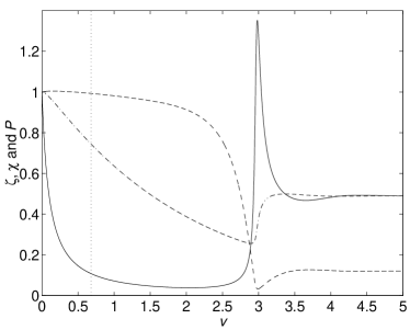
Figure 1: The values of $\zeta$ (continuous line), $\chi$ (dash-dotted line), and the purity (dashed line) as a function of time for simple feedback (27) with a spin of $j=5$. The vertical dotted line indicates the time at which the state is close to the optimal state considered for teleportation in Ref. Berry .

Recall that the system must be entangled if $\langle{(J_{z}^{(+)})^{2}+(J_{y}^{(-)})^{2}}\rangle<\langle{J_{x}^{(+)}}\rangle$ Berry , which is equivalent to $\zeta<\chi$. Therefore a state with $\zeta<\chi$ can be described as TMSS. Evidently the feedback produces quite strong spin squeezing. In order to determine how close to optimal the states produced by this feedback are, the value of $\zeta$ was plotted against $\chi$ and compared with the plot for optimal TMSS states in Fig. 2. As time progresses the state travels from the upper right corner towards the lower left corner of the figure.

The state starts out very close to optimum and does not deviate significantly from optimum until $\zeta<0.4$. Eventually the value of $\zeta$ increases dramatically, and the system spirals towards its equilibrium state at $(0.5,0.5)$. The results for $j=5$ are typical, and similar results are obtained for other spins $j>1/2$.

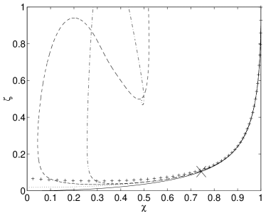
Figure 2: The values of $\zeta$ plotted against $\chi$ for spin $j=5$. The relation for optimal states is shown as the continuous line, the results for the simple feedback of Eq. (27) as the dash-dotted line, the analytic feedback of Eq. (36) as the dashed line, optimal feedback as the dotted line, and the countertwisting Hamiltonian (23) as the pluses. The cross shows the position of the optimal state considered for teleportation in Ref. Berry .

For the purposes of teleportation, the important issue is how close it is possible to get to the optimal TMSS states considered for teleportation in Ref. Berry . This state is indicated by the cross in Fig. 2. As can be seen, the states obtained by feedback closely approach this optimal state. Similar results are obtained for higher spin, but for smaller spin the states obtained by feedback are further from the TMSS states considered for teleportation.

The plots of $\zeta$ versus $\chi$ for analytic feedback and optimal feedback are also shown in Fig. 2. The results for analytic feedback are very similar to those for simple feedback, with $\zeta$ dramatically increasing at later times. In contrast, under optimal feedback the value of $\zeta$ monotonically decreases to an asymptotic value for $\chi=0$. For small times the three feedback schemes produce very similar results, and the states obtained using optimal feedback do not pass significantly closer to the optimal state for teleportation.

The last alternative that we consider in this section is the Hamiltonian (23), which is analogous to the two-axis countertwisting Hamiltonian in the single-mode case. The results for this Hamiltonian are also shown in Fig. 2. For this case there is significant spin squeezing, but the squeezing is generally poorer than for feedback. Nevertheless, at later times the value of $\zeta$ does not rise dramatically (until $\chi$ falls below zero), as opposed to the results for the simple or analytic feedback.

IV.2 Conditioned master equation

Next we consider the results for the conditioned master equation. There are two examples where it is necessary to consider the conditioned master equation. In the case of simple feedback, at the time that $\zeta$ increases dramatically the purity of the state has greatly decreased. This means that the feedback based on the unconditioned averages, Eq. (27), is a poor approximation of the feedback based on conditioned averages, Eq. (26), and will not accurately keep the average $\langle{J_{z}^{(\Omega)}}\rangle_{c}$ equal to zero. For this reason we may obtain better results using the conditioned master equation and the feedback (26).

The second case that we consider here is that without any feedback. In this case there is no reduction in the variances for the unconditioned equation. If we consider the conditioned equation, however, there is a reduction in the variances, though the means $\langle{J_{z}^{(+)}}\rangle_{c}$ and $\langle{J_{y}^{(-)}}\rangle_{c}$ are nonzero. For this reason we will consider the conditioned master equation for this case, with $\zeta$ defined by

$$\zeta=\frac{\langle{(J_{z}^{(+)}-\langle{J_{z}^{(+)}}\rangle_{c})^{2}+(J_{y}^{(-)}-\langle{J_{y}^{(-)}}\rangle_{c})^{2}}\rangle_{c}}{2j}.$$ (48)

To minimize the random differences between the two cases the same random numbers were used for each. The results for these two cases are plotted in Fig. 3.

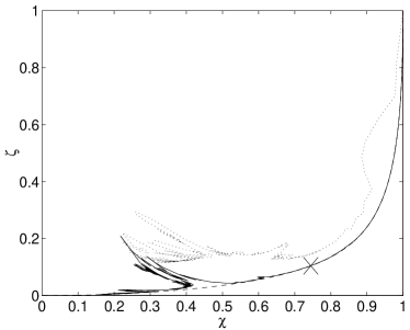
Figure 3: The values of $\zeta$ plotted against $\chi$ for spin $j=5$. The relation for optimal states is shown as the dashed line, the results for the feedback of Eq. (26) are shown as the continuous line, and without feedback as the dotted line. All results are for the conditioned master equation. The cross shows the position of the optimal state considered for teleportation in Ref. Berry .

The results for the feedback (26) are extremely close to the line for optimal states, with only temporary excursions from it. In particular, the value of $\zeta$ does not increase dramatically at large times. This indicates that improved results may be obtained using feedback based on the conditioned state.

On the other hand, implementing this feedback may be far more difficult. In the forms of feedback considered for the unconditioned equation, the feedback was proportional to the measurement record, with a proportionality constant $\lambda$ that is a function of time only. This feedback may be performed efficiently by calculating $\lambda(t)$ beforehand and programming it into a field programmable gate array FPGA . In contrast, the value of $\lambda$ given by Eq. (26) is dependent on the measurement record, and therefore would need to be calculated during the measurement, introducing a significant time delay.

The results without feedback quickly diverge from the line for optimal states, although they do not differ from it greatly. The major difference is at later times. While, with feedback, the value of $\zeta$ is reduced very close to zero, without feedback the value of $\zeta$ cannot be reduced as far. This means that, although a significant reduction in the variances can be achieved via feedback for strong QND measurements (where $\Gamma t>1$), feedback does not give much improvement for weak measurements.

V Comparison with single-mode case

There is clearly a great similarity between the single-mode and two-mode cases. The operators $J_{x}^{(+)}$, $J_{y}^{(\Omega)}$, and $J_{z}^{(\Omega)}$ obey exactly the same commutation relations as $J_{x}$, $J_{y}$, and $J_{z}$ in the single-mode case. This means that, for example, the optimal feedback also applies to the single-mode case (as was mentioned in Sec. III.3). As we may replace the sum of the variances $\langle{(J_{z}^{(+)})^{2}+(J_{y}^{(-)})^{2}}\rangle$ with $2\langle{(J_{z}^{(\Omega)})^{2}}\rangle$, it might appear that this case is identical to the single-mode case. Nevertheless, there is a subtle difference due to the fact that the operator $J_{z}^{(\Omega)}$ is time dependent.

For the case of spin 1/2, there is complete equivalence between the single-mode case (for spin $j=1$) and the two-mode case. We will take the Hilbert space for the single-mode case to be that for two spin 1/2 particles, so that it is the same as for the two-mode case. The optimal TMSS states for $j=1/2$ are also optimal single-mode squeezed states in terms of the total spin. That is, they minimize $\langle{(J_{z}^{(+)})^{2}}\rangle$ for a given $\langle{J_{x}^{(+)}}\rangle$. The converse is also true: the states optimized for single-mode spin squeezing are automatically optimized for two-mode spin squeezing.

In addition, both the single- and two-mode countertwisting Hamiltonians produce optimal spin squeezed states. Not only this, but the feedback as given by Eq. (28) in the single-mode case, or Eq. (27) in the two-mode case, and the optimal feedback described in Sec. III.3, give optimal spin squeezed states. The only feedback that does not give optimal states is the analytic feedback for the single- or two-mode case. These results are depicted in Fig. 4. In this figure the variables $\zeta$ and $\chi$ are defined for the single-mode case as

$$\zeta=2\langle{J_{z}^{2}}\rangle/j,~{}~{}~{}~{}~{}~{}\chi=\langle{J_{x}}\rangle/j.$$ (49)

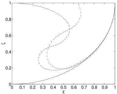
Figure 4: The values of $\zeta$ plotted against $\chi$ for spin $j=1/2$ in the two-mode case and $j=1$ in the single-mode case. The relation for optimal states, single- or two-mode countertwisting, the feedbacks of Eq. (28) in the single-mode case and Eq. (27) in the two-mode case, and the optimal feedback of Sec. III.3, are shown as the continuous line. The results for the analytic feedback of Eq. (36) in the two-mode case, and Eq. (31) in the single-mode case are shown as the dashed line and dash-dotted line, respectively.

To explain these results analytically, first note that, for spin 1/2,

$$J_{z}^{(+)}J_{y}^{(+)}+J_{y}^{(+)}J_{z}^{(+)}=2(J_{z}^{(1)}J_{y}^{(2)}+J_{y}^{(1)}J_{z}^{(2)}).$$ (50)

This means that the countertwisting Hamiltonians for the one- and two-mode cases are identical, and therefore produce identical states.

In addition we find that $(J_{z}^{(+)})^{2}-(J_{y}^{(-)})^{2}$ commutes with these Hamiltonians. This means that for the states produced by countertwisting, the values of $\langle{(J_{z}^{(+)})^{2}}\rangle$ and $\langle{(J_{y}^{(-)})^{2}}\rangle$ will be identical. This means that, if the states produced are optimal single-mode spin squeezed states (i.e., $\langle{(J_{z}^{(+)})^{2}}\rangle$ is minimized), then they must also be optimal TMSS states.

To show that optimal single-mode spin squeezed states are produced by the countertwisting Hamiltonian, note that for total spin 1 we have the differential equations

$$\frac{d}{dv}\langle{J_{x}}\rangle =2\langle{J_{z}^{2}-J_{y}^{2}}\rangle,$$ (51)

$$\frac{d}{dv}\langle{J_{z}^{2}}\rangle =-\langle{J_{x}}\rangle,$$ (52)

$$\frac{d}{dv}\langle{J_{y}^{2}}\rangle =\langle{J_{x}}\rangle.$$ (53)

The solution of these equations is

$$\langle{J_{x}}\rangle^{2}=4(\langle{J_{z}^{2}}\rangle-\langle{J_{z}^{2}}\rangle^{2}).$$ (54)

This is the relation for optimal single-mode spin squeezed states as given by Sørensen and Mølmer Sor01 . This shows that the states produced by the one- and two-mode countertwisting Hamiltonians and the one- and two-mode optimal states are all identical.

For the case of feedback, it is sufficient to show that the feedbacks of Eqs. (28) and (27) give optimal states, as this will imply that the optimal feedback gives optimal spin squeezed states. The derivation in this case is lengthy, and is given in Appendix B. It is interesting to note that in this case the optimal feedback is given by Eq. (65), and differs dramatically from the analytic feedback used for higher spin.

The equivalence between the single- and two-mode cases does not hold for any total spin higher than 1. As shown in Fig. 5, there are significant differences between the optimal single- and two-mode spin squeezed states for total spin above 1. As can be seen, for a total spin of 2 or more the values of $\zeta$ are significantly less for the single-mode case than for the two-mode case. This reflects the fact that in the two-mode case we wish to minimize $\langle{(J_{y}^{(-)})^{2}}\rangle$ as well as $\langle{(J_{x}^{(+)})^{2}}\rangle$.

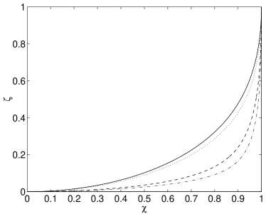
Figure 5: The values of $\zeta$ for optimal states plotted against $\chi$ for total spin 2 for the two-mode case (continuous line) and the single-mode case (dotted line), and for total spin 10 for the two-mode case (dashed line) and the single-mode case (dash-dotted line).

As there are such strong similarities between the single-mode and two-mode cases, it is reasonable to apply the squeezing parameter as considered in Refs. Laura ; Sorensen ; Wang to the two-mode case. In the single-mode case the squeezing parameter was defined by

$$\xi_{z}^{2}=2j\langle{J_{z}^{2}}\rangle/\langle{J_{x}}\rangle^{2}.$$ (55)

With the definitions of $\zeta$ and $\chi$ for the single-mode case above, this can be expressed as $\xi_{z}^{2}=\zeta/\chi^{2}$. It would seem reasonable to use the same definition for the two-mode case.

For the two-mode case we find that the minimum value of $\xi_{z}^{2}$, namely $\xi_{\rm min}^{2}$, varies with spin $j$ as shown in Fig. 6(a). In this figure the values of $\xi_{\rm min}^{2}$ have been multiplied by $j+1$ in order to more easily compare the results for different spins. Very similar results are obtained for the simple feedback of Eq. (27) and the optimal feedback of Eq. (46). Using the analytic feedback of Eq. (36) gives results that are similar to, but slightly above, those for the other two feedback schemes. All of these feedback schemes give results that are significantly above the result for the optimal states. Using the countertwisting Hamiltonian (23) gives results that are higher than those for feedback.

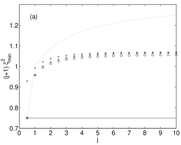
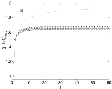
Figure 6: The minimum squeezing parameter $\xi_{\rm min}^{2}$ multiplied by $j+1$ as a function of $j$ in the two-mode case (a) and the single-mode case (b) for optimal states (continuous line), the feedbacks of Eqs. (27) and (28) for (a) and (b), respectively (crosses), analytic feedback (pluses), optimal feedback (circles), and countertwisting (dotted line).

Similar results are obtained for the single-mode case [see Fig. 6(b)]. The results for feedback are noticeably above those for optimal states, and the results for two-axis countertwisting are significantly above those for feedback. To summarize, the scaling constants for each of the cases are as given in Table 1. In this table we can see the similarities between the single-mode and two-mode cases: the scaling constants obtained by feedback are significantly above those for optimal states, and the scaling constants for two-axis countertwisting (or its two-mode equivalent) are significantly above those for feedback. In both cases there are only small differences between the results for the different types of feedback. The only qualitative difference between the scaling constants for the single- and two-mode cases are that in the single-mode case the analytic feedback gives slightly better results than the simple feedback of Eq. (27). In contrast, in the two-mode case the scaling constants are indistinguishable.

Table 1: The scaling constants for the minimum squeezing parameter $\xi_{\rm min}^{2}$ for both single- and two-mode spin squeezing, for optimal states, simple feedback, analytic feedback, optimal feedback, and two-axis countertwisting (or its equivalent in the two-mode case).

	Optimal	Optimal feedback	Analytic feedback	Simple feedback	Countertwisting
Single mode	1	1.6468	1.6593	1.6777	1.9562
Two mode	3/4	1.0584	1.0692	1.0692	1.292

VI Experimental prospects

There are some complications in applying this theory to the experiment of Ref. Julsgaard . In this experiment, $a\approx 5\times 10^{-13}$, and $\nu\approx 2\times{10^{16}}{\rm s}^{-1}$. This means that $\Gamma\approx{1.4}\times{10^{-9}}{\rm s}^{-1}$, which implies that the time required for maximal squeezing is on the order of $10^{9}{\rm s}$ (over 20 yr). Therefore a far more intense beam or a stronger interaction would be required to obtain the two-mode spin squeezing described here.

It must be emphasized that this long time is required for the measurements, not the feedback. Feedback may be applied to the states obtained in Ref. Julsgaard with a negligible increase in the time required for the experiment. Nevertheless, for the conditions of this experiment, although the feedback will bring the means of $J_{z}^{(+)}$ and $J_{y}^{(+)}$ towards zero, it will not significantly reduce the variances. It is only when the QND measurement can be performed strongly enough (i.e., with a strong enough interaction over a long enough time) to obtain spin squeezing close to maximum that an improvement in the variance is obtained by using feedback.

Another problem is spontaneous losses due to absorption of QND probe light. The loss rate due to this is $N\gamma g^{2}n/4\Delta^{2}$, where $N=4j$ is the total number of atoms and $g$ is the one-photon Rabi frequency. As in the case of single-mode spin squeezing Laura , this loss will be very large over the time period $1/\Gamma$ for free space. Both this problem and the problem of the long interaction time may be overcome by performing the experiment in a cavity in the strong-coupling regime.

Two other common experimental problems are inefficient detectors and time delays. As for the case of single-mode spin squeezing, inefficient detectors do not affect the scaling. The system has the potential to be far more sensitive to time delays than in the single-mode case, however. The problem is that, as the spin component that is being measured is rotating rapidly, the feedback may be correcting for measurements of a different spin component.

In order to correct the right spin component, the rotation of the spin component that is measured should have completed an integral number of rotations during the time delay. Experimentally, this means that the magnetic field should be adjusted such that the frequency $\Omega$ is an integral multiple of $2\pi/\tau$, where $\tau$ is the time delay. Provided that this is done, time delays should not be more of a problem than in the single-mode case.

VII Conclusions

Two-mode spin squeezed states are important states to produce for quantum teleportation. Here we have shown that it is possible to produce states very close to the optimal TMSS states by adapting the feedback for single-mode spin squeezing considered by TMW. These states are not conditioned on the measurement record, in contrast to the conditional two-mode spin squeezing discussed in Ref. Julsgaard .

Using the simple feedback scheme (27) it is possible to obtain states that are quite close to optimal TMSS states for small times, but strongly diverge from these states at later times. In particular, for spins above about 5 it is possible to obtain states very close to the TMSS states considered for teleportation in Ref. Berry . An analytic feedback scheme (36) also gives similar results. This feedback scheme is more practical experimentally, as the appropriate feedback strength to be used is easily calculated.

We have derived the optimal feedback that produces the maximum possible spin squeezing. This feedback is also applicable to the case of feedback for single-mode spin squeezing. This feedback gives states even closer to the optimal TMSS states.

We have also derived a Hamiltonian for the two-mode case that is equivalent to the two-axis countertwisting Hamiltonian introduced in Ref. Kit . This Hamiltonian produces spin squeezing, but not as strongly as the measurements with feedback.

In the case of spin 1/2 both the feedback (except for the analytic feedback) and the countertwisting Hamiltonian produce optimal TMSS states. These states are equivalent to optimal single-mode spin squeezed states if the two modes are considered as a single spin-1 system. In the single-mode case optimal spin squeezed states are produced both by feedback and by the countertwisting Hamiltonian.

Appendix A Relation of variables to experiment

Here we give further explanation of the variables introduced in Eq. (1). The coupling constant $a$ is given by

$$a=\frac{\sigma}{A(I+1/2)}\frac{\gamma}{\Delta}\alpha_{v},$$ (56)

where $\sigma$ is the resonant absorption cross section, $A$ is the area of the transverse cross section of the light beam, $I$ is the nuclear spin, $\gamma$ is the spontaneous emission rate of the upper atomic level, $\Delta$ is the detuning, and $\alpha_{v}$ is the dynamic vector polarizability. We have omitted the bounds on the integral (1) for greater generality, so we may apply this expression to multiple samples. Explicit bounds are unnecessary, as there is no contribution to the integral from regions where there are no atoms.

The continuous spin operators for the sample are defined as

$$J_{k}(z,t)=\lim_{\delta z\to 0}\frac{1}{\delta z}\sum_{\mu}\tfrac{1}{2}\sigma_{k}^{\mu},$$ (57)

where $k\in\{x,y,z\}$ and $\sigma_{k}^{\mu}$ is the Pauli operator for particle $\mu$. The sum is over all particles between $z$ and $z+\delta z$ over the cross section of the sample. The operator for the entire sample is obtained by integrating over $z$.

The field is described by the continuous-mode annihilation operators $a_{k}(z,t)$, where $k=x$ and $y$ for the $x$ polarized and $y$ polarized modes, respectively. The instantaneous Stokes parameters are

$$S_{x}(z,t) =\tfrac{1}{2}[a_{x}^{\dagger}(z,t)a_{x}(z,t)-a_{y}^{\dagger}(z,t)a_{y}(z,t)],$$

$$S_{y}(z,t) =\tfrac{1}{2}[a_{x}^{\dagger}(z,t)a_{y}(z,t)+a_{y}^{\dagger}(z,t)a_{x}(z,t)],$$

$$S_{z}(z,t) =-\frac{i}{2}[a_{x}^{\dagger}(z,t)a_{y}(z,t)-a_{y}^{\dagger}(z,t)a_{x}(z,t)].$$ (58)

The Stokes vector for the entire pulse at position $z$ is given by ${\bf S}(z)=\int{\bf S}(z,t)dt$.

Appendix B Feedback for total spin 1

Here we show that the feedback of either Eqs. (28) or (27) gives optimal spin squeezed states for a total spin of 1. To see this, note first that the first term in Eq. (19) is just the same as that produced by the countertwisting Hamiltonian, and so will produce optimal states. In order to show that the feedback produces optimal states, it remains to be shown that the second term, ${\cal D}[c-iF]\rho$, does not alter the evolution. Specifically, in the single-mode case

$${\rm Tr}\left\{J_{x}{\cal D}[J_{z}-i\Lambda J_{y}]\rho\right\}=-\tfrac{1}{2}(1+\Lambda^{2})\langle{J_{x}}\rangle+\Lambda\langle{J_{z}^{2}+J_{y}^{2}}\rangle.$$ (59)

If the state $\rho$ is an optimal state, then $\langle{J_{z}^{2}+J_{y}^{2}}\rangle=1$, so this simplifies to

$${\rm Tr}\left\{J_{x}{\cal D}[J_{z}-i\Lambda J_{y}]\rho\right\}=-\tfrac{1}{2}(1+\Lambda^{2})\langle{J_{x}}\rangle+\Lambda.$$ (60)

Similarly we can show that

$${\rm Tr}\left\{J_{z}^{2}{\cal D}[J_{z}-i\Lambda J_{y}]\rho\right\}=-\frac{\Lambda}{2}\langle{J_{x}}\rangle+\Lambda^{2}\langle{J_{x}^{2}-J_{z}^{2}}\rangle.$$ (61)

For optimal states, $\langle{J_{x}^{2}}\rangle=1$, so this becomes

$${\rm Tr}\left\{J_{z}^{2}{\cal D}[J_{z}-i\Lambda J_{y}]\rho\right\}=-\frac{\Lambda}{2}\langle{J_{x}}\rangle+\Lambda^{2}(1-\langle{J_{z}^{2}}\rangle).$$ (62)

It is simple to show that both Eqs. (60) and (62) will be zero if Eq. (54) is satisfied, and the feedback is given by Eq. (28).

Therefore, if the state is already in an optimal state, and the feedback as given by Eq. (28) is used, then the state will continue to be in an optimal state. On the other hand, if some other feedback is used, then optimal states will not be obtained. For example, the analytic feedback considered by LMW does not give optimal states. In order to determine analytic feedback that will give optimal states, note that the differential equations for $\langle{J_{x}}\rangle$ and $\langle{J_{z}^{2}}\rangle$ are

$$\frac{d}{dv}\langle{J_{x}}\rangle =\Lambda(2\langle{J_{z}^{2}}\rangle-1),$$

$$\frac{d}{dv}\langle{J_{z}^{2}}\rangle =-\frac{\Lambda}{2}\langle{J_{x}}\rangle.$$ (63)

Solving these using the feedback (28) and Eq. (54) gives

$$\left\langle{J_{x}}\right\rangle =\sqrt{2e^{-v}-e^{-2v}},$$

$$\left\langle{J_{z}^{2}}\right\rangle =\tfrac{1}{2}e^{-v}.$$ (64)

This implies that the value of $\Lambda$ should change with time as

$$\Lambda(v)=\frac{1}{\sqrt{2e^{v}-1}}.$$ (65)

This is quite different from the analytic expression applied for larger spins.

The case for feedback for two-mode spin squeezing is analogous to this, except that $J_{x}$, $J_{y}$, and $J_{z}$ are replaced with $J_{x}^{(+)}$, $J_{y}^{(\Omega)}$, and $J_{z}^{(\Omega)}$. This therefore shows that optimal states are obtained in the one- and two-mode cases using the feedback given by Eqs. (28) and (27), respectively.

References

- (1) B. Julsgaard, A. Kozhekin, and E. S. Polzik, Nature (London) 413, 400 (2001).
- (2) A. Kuzmich and E. S. Polzik, Phys. Rev. Lett. 85, 5639 (2000).
- (3) D. W. Berry and B. C. Sanders, New J. Phys. 4, 8 (2002).
- (4) M. A. Nielsen and I. L. Chuang, Quantum Computation and Quantum Information (Cambridge University Press, Cambridge, England, 2000).
- (5) C. M. Caves and B. L. Schumaker, Phys. Rev. A31, 3068 (1985).
- (6) A. Furusawa, J. L. Sørensen, S. L. Braunstein, C. A. Fuchs, H. J. Kimble, and E. S. Polzik, Science 282, 706 (1998).
- (7) A. S. Sørensen and K. Mølmer, Phys. Rev. Lett. 86, 4431 (2001).
- (8) H. M. Wiseman and G. J. Milburn, Phys. Rev. A49, 1350 (1994).
- (9) L. K. Thomsen, S. Mancini, and H. M. Wiseman, Phys. Rev. A 65, 061801(R) (2002).
- (10) H. M. Wiseman and R. B. Killip, Phys. Rev. A57 2169, (1998).
- (11) D. W. Berry and H. M. Wiseman, Phys. Rev. A63 013813, (2001).
- (12) A. Kuzmich, L. Mandel, J. Janis, Y. E. Young, R. Ejnisman, and N. P. Bigelow, Phys. Rev. A60, 2346 (1999).
- (13) T. Holstein and H. Primakoff, Phys. Rev. 58, 1098 (1940).
- (14) R. T. Sang, G. S. Summy, B. T. H. Varcoe, W. R. MacGillivray, and M. C. Standage, Phys. Rev. A 63, 023408 (2001).
- (15) H. M. Wiseman, Phys. Rev. A49, 2133 (1994).
- (16) M. Kitagawa and M. Ueda, Phys. Rev. A47, 5138 (1993).
- (17) J. Stockton, M. Armen, and H. Mabuchi, quant-ph/0203143, 2002 (unpublished).
- (18) A. Sørensen, L.-M. Duan, J. I. Cirac, and P. Zoller, Nature (London) 409, 63 (2001).
- (19) X. Wang, J. Opt. B: Quantum Semiclassical Opt. 3, 93 (2001).