Strange attractor simulated on a quantum computer

Abstract

We show that dissipative classical dynamics converging to a strange attractor can be simulated on a quantum computer. Such quantum computations allow to investigate efficiently the small scale structure of strange attractors, yielding new information inaccessible to classical computers. This opens new possibilities for quantum simulations of various dissipative processes in nature.

Starting from the work of Lorenz lorenz , it has been realized that the dynamics of many various dissipative systems converges to so-called strange attractors ruelle . These objects are characterized by fractal dimensions and chaotic unstable dynamics of individual trajectories (see e.g. ott ; lichtenberg ). They appear in nature in very different contexts, including applications to turbulence and weather forecast lorenz ; ruelle , molecular dynamics hoover , synchronization pikovsky , chaotic chemical reactions belousov , multimode solid state lasers roy and complex dynamics in ecological systems ecology ; plankton and physiology glass . The efficient numerical simulation of such dissipative systems can therefore lead to many important practical applications.

Recently, it has been understood that quantum mechanics allows to perform computations in a fundamentally new way (see for review e.g. divi ; ekert ; steane ; preskill ; nielsen ). Indeed, quantum parallelism can enormously accelerate the computation and provide new information inaccessible to classical computers. Well-known examples are Shor’s factorization algorithm shor , which is exponentially faster than any known classical method, and Grover’s search algorithm grover , where the gain is polynomial. Even if important progress has been achieved during the last years, still it is essential to find new areas where quantum processors might give access to new information unreachable classically. Especially interesting are applications to dissipative systems with irreversible dynamics leading to a loss of information.

In this Letter we analyze how classical dissipative dynamics can be simulated on such quantum processors. To this aim, we study a simple deterministic model where dynamics converges to a strange attractor, and show that it can be efficiently simulated on a quantum computer. Even if the dynamics on the attractor is unstable, dissipative and irreversible, a realistic quantum computer divi ; ekert ; steane ; preskill ; zoller ; kane can simulate it in a reversible way, and, already with 70 qubits, will provide access to new informations inaccessible for modern supercomputers.

To study how a quantum computer can simulate dissipative dynamics leading to a strange attractor, we choose the deterministic map given by:

$$\bar{y}=y/2+x\;\mbox{(mod}\;\mbox{2)}\;\;,\;\;\bar{x}=x+\bar{y}\;\mbox{(mod}\;\mbox{1)}\;.$$ (1)

where $-0.5\leq x<0.5$, $-1\leq y<1$ and bars note the new values of variables. The map has one positive $\lambda_{+}$ and one negative $\lambda_{-}$ Lyapunov exponents ($\lambda_{\pm}=\ln[(5\pm\sqrt{17})/2]$) so that the dynamics converges to a strange attractor with Hausdorff ($D_{H}$) and information ($D_{I}$) dimensions kaplan ; grassberger ; procaccia $D_{H}\approx D_{I}=1+\lambda_{+}/|\lambda_{-}|\approx 1.543$.

To implement this map for a computer simulation it is necessary to discretize the phase space. We choose the natural discretization in the binary representation of coordinates $(x,y)$, so that the dynamics takes place on a regular square lattice with $N\times 2N$ points, with $N=2^{n_{q}}$ and $n_{q}$ integer. The division in (1) is realized by shift and truncation of the last binary digit. With this procedure, the dissipation generates a discretized irreversible map, displaying a discretized strange attractor (see Fig.1 top) which approaches the continuous one for large $N$. Such a map can be implemented efficiently on a quantum computer. For that, an initial image with $N_{d}$ points is coded in the wave function $|\Psi_{0}>=\sum_{i,j}a_{ij}|x_{i}>|y_{j}>|0>|0>$, where $a_{i,j}=0$ or $1/\sqrt{N_{d}}$. Here the two registers $|x_{i}>$ and $|y_{j}>$ with $n_{q}$ and $n_{q}+1$ qubits hold the values of the coordinates $x$ and $y$ ($x_{i}=-0.5+i/N,i=0,...,N-1$ and $y_{j}=-1+j/N,j=0,...,2N-1$). The third register with $n_{q}-1$ qubits is used as workspace for modular additions, and the last one collects the truncated last digits generated by the divisions (“garbage”). We start with the simplified algorithm for which the garbage gets one digit at each map iteration so that $t$ iterations need $t$ qubits in the fourth register. The size of this register can be significantly reduced using a more refined algorithm we will describe later.

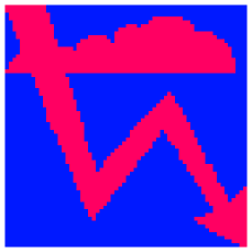
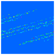
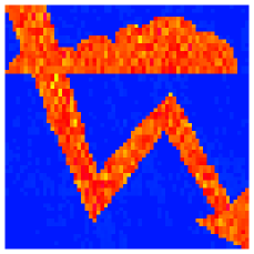
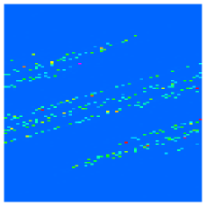
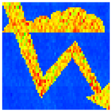
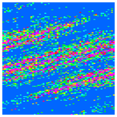
Figure 1: (color) Top: exact classical/quantum computation of the discretized map (1); initial image (left) converged to the strange attractor after $t=10$ iterations (right). Middle: quantum computation with noise amplitude $\epsilon=0.05$ in each gate operation; attractor at $t=10$ (right) and initial image recovered after $10$ backwards iterations with fidelity $f=0.63$ (left). Bottom: same as middle with $\epsilon=0.1$ and $f=0.15$. Left shows the central cell ($-0.5\leq x,y<0.5$), right shows the whole phase space. Color marks the probability density (integrated over third and fourth registers), from blue (density less than $10^{-5}$) to red (maximal value). Here $n_{q}=6$, with in total $28$ qubits used.

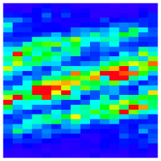
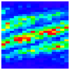
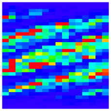
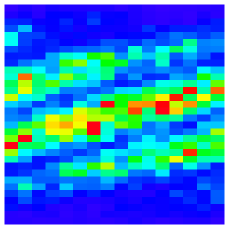
Figure 2: (color) Spectral density $|C(t,k_{x,y})|^{2}$ for the strange attractor of Fig.1 at $t=10$ in the region $-N/2\leq k_{x}\leq N/2$, $-N\leq k_{y}\leq N$ ($N=2^{n_{q}}$). Top: three-dimensional plot of the full distribution for $n_{q}=6$ and $\epsilon=0$ (left), $\epsilon=0.025$ (right). Middle: color plot of the coarse-grained distribution with $n_{q}=6$, $n_{f}=4$ and $\epsilon=0$ (left), $\epsilon=0.025$ (right). Bottom: same as middle for $n_{q}=10$, $\epsilon=0$ (left), and $n_{q}=6$, $\epsilon=0.05$ (right). Colors are as in Fig.1.

The algorithm starts with the initial state $|\Psi_{0}>$; first it places the last qubit of $|y>$ in the garbage register, and uses $n_{q}$ swap gates to shift the $|y>$ qubits and obtain $y/2$. Then a modular addition is implemented in the way described in barenco to add $x$ to $y/2$. After that, another modular addition adds the second register to the first. In total, this requires $17n_{q}-10$ quantum operations using Toffoli, control-not and swap gates in contrast to $O(2^{2n_{q}})$ operations for the classical algorithm. It is interesting to note that the algorithm allows to restore the initial state: inverse map iterations are performed ($x=\bar{x}-\bar{y}$, $y/2=\bar{y}-x$) and $y$ is restored from $y/2$ using a qubit stored in the garbage register. This requires a similar number of operations as the forward iterations. In principle this can be done on a classical computer in $O(2^{2n_{q}})$ operations, but this requires additional exponentially large memory which stores about $2^{2n_{q}}t$ bits for $N_{d}\sim N^{2}$, contrary to only $t$ qubits used by the quantum computer.

Fig.1 shows the dynamics generated by the discretized map (1) simulated on a quantum computer with exact and noisy unitary gates with imprecisions of amplitude $\epsilon$. Due to the dissipative nature of the map (1), the initial image rapidly converges towards the strange attractor (already $t=5$ is enough). Even in the presence of relatively strong noise, the fractal structure of the attractor is well-preserved and the initial image can be reliably recovered after backwards iterations, despite the exponential instability of the classical dynamics (1). The precision of computation can be quantitatively characterized through the fidelity $f$ defined at a given moment of time as the projection of the quantum state in presence of gate imperfections on the exact state without imperfections. The global properties of the initial image can be recovered even at relatively low fidelity values.

Even if the quantum algorithm performs one map iteration only in $O(n_{q})$ operations, it is important to take into account the measurement procedure that allows to extract efficiently the information coded in the wave function. Indeed the number of points in Fig.1 grows exponentially with $n_{q}$ and an exponential number of measurements is required to obtain the full density distribution. However, certain characteristics can be extracted in a polynomial number of measurements, providing new information inaccessible for classical computation. An example of such a quantity is the spectrum of phase space correlation functions, defined as $C(t,k_{x,y})=\sum_{x_{0},y_{0}}\exp(2i\pi(x(t,x_{0},y_{0})+y(t,x_{0},y_{0})))\exp(2i\pi(k_{x}x_{0}+k_{y}y_{0}))$, where the sum runs over the points $(x_{0},y_{0})$ of the initial distribution, and $(x(t,x_{0},y_{0}),y(t,x_{0},y_{0}))$ is the position of $(x_{0},y_{0})$ at time $t$. Such correlation functions have been studied for chaotic systems, where they determine various kinetic coefficients, for example the diffusion rate (see e.g. lichtenberg p.328). Due to chaos, the function $C(t,k_{x,y})$ has significant values at exponentially high harmonics $k_{x,y}\sim\exp(|\lambda_{-}|t)$ which rapidly reaches harmonics of order $N$. In the theory of classical chaotic dynamics it is well-known that the information about such harmonics is very hard to access, since exponentially small scales should be explored, which can be done only with exponentially many trajectories lichtenberg ; peres . On the contrary, the quantum computation of $C(t,k_{x,y})$ can be done efficiently. For that, one makes $t$ iterations of (1), and creates the state $\sum a_{x,y}\exp(2i\pi(x+y))|x>|y>|0>|g(t)>$. The preparation of this state is easily done by applying $2n_{q}+1$ one-qubit rotations to the first two registers. Then the garbage $g(t)$ is erased by iterating the map backwards $t$ times, that at the same time returns the coefficients $a_{x,y}$ to their original values. This creates the state $\sum a_{x_{0},y_{0}}\exp(2i\pi(x(t,x_{0},y_{0})+y(t,x_{0},y_{0}))|x_{0}>|y_{0}>|0>|0>$, keeping phases unchanged. The whole procedure is sometimes called “phase kickback”. After that the application of a two-dimensional quantum Fourier transform ekert yields in $O(n_{q}^{2})$ operations the state $\sum C(t,k_{x,y})|k_{x}>|k_{y}>|0>|0>$. A polynomial number of measurements yields the principal peaks, or enables to obtain a coarse-grained image of the spectral density $|C(t,k_{x,y})|^{2}$ in the Fourier space. Indeed, independently of $n_{q}$, one can measure the first $n_{f}$ and $n_{f}+1$ qubits of the $x$ and $y$ registers respectively, that gives integrated probability inside $2^{2n_{f}+1}$ cells. Fig.2 displays the spectral density for the case of Fig.1. It shows that new information about the coarse-grained spectral density can be obtained efficiently. Indeed, patterns are clearly present in Fig.2 and they vary irregularly with $n_{q}$ (compare Fig.2 middle left and bottom left). This confirms the nontrivial nature of information provided by the coarse-grained density $|C(t,k_{x,y})|^{2}$. Although the spectral density is more sensitive to noise than the distribution in Fig.1 still the patterns remain well-defined even in the presence of relatively strong errors (see Fig.2).

It is important to stress that even modern supercomputers are unable to find the properties of the spectral density for $n_{q}\geq 20$. Indeed, as is shown in Fig.3, a classical Monte Carlo algorithm requires an exponentially large number of trajectories $M$ ($M=O(2^{2n_{q}})$) to obtain the coarse-grained spectral density at fixed $n_{f}$ with fixed accuracy. In contrast, the quantum computation requires a number of measurements $M$ independent of $n_{q}$ (each measurement is done after $t$ map iterations and one Fourier transform which needs $O(n_{q}^{2})$ quantum gates).

Figure 3: Complexity of classical and quantum computations of coarse-grained distribution of Fig.2 with 10% accuracy (i.e. fidelity $f(t)=0.9$). Here $n_{f}=4,t=10$ and different values of $n_{q}$ are shown. For classical computation (open circles), $M$ gives the number of classical Monte Carlo trajectories required to reach 10% accuracy. For quantum case (full circles), $M$ is the number of measurements needed to obtain the same accuracy. Full line shows the total number of classical points in the initial image shown in Fig.1 ($M\approx 0.36\times 2^{2n_{q}}$). Logarithm is decimal.

To study the effect of noisy gates in a more quantitative way, we show in Fig.4 the dependence of the fidelity $f(t)$ of the quantum computation of spectral amplitudes $C(t,k_{x,y})$ on the noise amplitude $\epsilon$ and total number of gates $n_{g}$ applied ($n_{g}=t(44n_{q}-14)+(n_{q}+2)^{2}-2$). The data show the global scaling law $1-f(t)\approx\epsilon^{2}n_{g}/14$, valid for moderate $\epsilon$. The physical origin of this scaling law is related to the fact that for randomly fluctuating unitary gates the loss of probability from the exact state is of the order of $\epsilon^{2}$ for each gate operation. This law determines a time scale $t_{f}\approx 1/(6\epsilon^{2}n_{q})$ up to which a reliable quantum computation is possible ($f\geq 0.5$). Beyond $t_{f}$ the decoherence destroys the accuracy of the quantum computation and the results become strongly distorted, see e.g. Fig.2 bottom right. We note that a similar time scale appears in quantum computation of Shor’s algorithm on a realistic quantum computer zurek . The computation beyond the scale $t_{f}$ is possible but requires the application of quantum error-correcting codes, at the cost of additional qubits and gates (see e.g. steane ; preskill and refs. therein). Without error correction, it is still possible to improve the fidelity of the final state by measuring the third and fourth registers. Indeed for exact computation they are at zero after the backwards iterations while with noisy gates the error probability grows as $W_{g}\approx 3.5\epsilon^{2}t$ (Fig.4 inset). The measurements of these registers allow to select the correct states and increase the fidelity by a factor $1/(1-W_{g})$, e.g. for the case of Fig.1 bottom this procedure gives $f=0.22$.

Figure 4: Fidelity $f$ for the spectral amplitudes of Fig.2 as a function of $\epsilon^{2}n_{g}$ for $4\leq n_{q}\leq 6$, $10^{-4}\leq\epsilon\leq 0.5$ and $6\leq t\leq 10$. Inset: error probability $W_{g}$ in the third and fourth registers as a function of $\epsilon^{2}t$ for $n_{q}=6$. Straight lines show the theoretical slope $1$, logarithms are decimal.

The above algorithm is optimal for not very large times $t$. If one is interested in simulating the dynamics on the attractor for large $t$, then the size of the garbage register can be significantly reduced. Indeed, at any $t$, copying the results $x(t),y(t)$ in two additional registers and reversing the sequence of gates allows to erase the garbage and reproduce $x_{0},y_{0}$. This procedure can be done recursively following the strategy of “reversible pebble game”, the description of which can be found in preskill . In the simplest version, $n_{t}$ qubits in the garbage register (plus the two additional registers for $x_{0},y_{0}$) allow to perform map iterations up to $t\sim 2^{n_{t}}$. This gives only a polynomial increase in the number of elementary quantum operations, being proportional to $n_{g}^{1.58}$. The procedure becomes cost-effective for $t\gg n_{q}$.

The algorithm described above can be generalized to other dissipative maps. For example, modular multiplications can be performed in $O(n_{q}^{2})$ operations, as described in barenco . This allows to simulate efficiently the map (1) with $x^{2}$ term in first equation and also the Hénon attractor $\bar{x}=y+1-ax^{2},\;\bar{y}=bx$ lichtenberg . Such an algorithm can also be adapted to perform the finite-step integration of the Lorenz system $\dot{x}=-\sigma(x-y),\;\dot{y}=-xz+rx-y,\;\dot{z}=xy-bz$ lorenz . However the simulation of the dissipative dynamics of these models requires more qubits than for (1).

Thus on the example of the map (1), we have shown that a quantum computer can efficiently simulate dissipative irreversible dynamics. A quantum processor with 70 qubits will be able to provide new information about small-scale structures of strange attractors inaccessible to modern supercomputers.

We thank CalMiP in Toulouse and IDRIS in Orsay for access to their supercomputers which were used to simulate quantum computations. This work was supported in part by the EC RTN contract HPRN-CT-2000-0156 and also by the NSA and ARDA under ARO contract No. DAAD19-01-1-0553.

References

- (1) E. N. Lorenz, J. Atmos. Sciences 20, 130 (1963).
- (2) D. Ruelle, and F. Takens, Comm. Math. Phys. 20, 167 (1971).
- (3) E. Ott, Chaos in dynamical systems, Cambridge Univ. Press (1993).
- (4) A. Lichtenberg, and M. Lieberman, Regular and chaotic dynamics, Springer, N.Y., (1992).
- (5) W. G. Hoover, Time reversibility, computer simulation, and chaos, World Scientific, Singapore, (1999).
- (6) A. Pikovsky, M. Rosenblum and J. Kurths, Synchronization: a universal concept in nonlinear sciences, Cambridge Univ. Press (2001).
- (7) R. A. Schmitz, K. R. Graziani, and J. L. Hudson, J. Chem. Phys. 67, 3040 (1977).
- (8) C. Bracikowski, and R. Roy, Chaos 1, 49 (1991).
- (9) B. Blasius, A. Huppert, and L. Stone, Nature 399, 354 (1999).
- (10) J. Huisman, and F. J. Weissing, Nature 402, 407 (1999).
- (11) L. Glass, Nature 410, 277 (2001).
- (12) D. P. DiVincenzo, Science 270, 255 (1995).
- (13) A. Ekert, and R. Josza, Rev. Mod. Phys. 68, 733 (1996).
- (14) A. Steane, Rep. Progr. Phys. 61, 117 (1998).
- (15) J. Preskill, Quantum information and computation, http://www.theory.caltech.edu/people/preskill/ph229/.
- (16) M. A. Nielsen, and I. L. Chuang, Quantum computation and quantum information, Cambridge Univ. Press (2000).
- (17) P. W. Shor, in Proc. 35th Annu. Symp. Foundations of Computer Science (ed. Goldwasser, S. ), 124 (IEEE Computer Society, Los Alamitos, CA, 1994).
- (18) L. K. Grover, Phys. Rev. Lett. 79, 325 (1997).
- (19) J. I. Cirac and P. Zoller, Phys. Rev. Lett. 74, 4091 (1995).
- (20) B. E. Kane, Nature 393, 133 (1998).
- (21) J. L. Kaplan, and J. A. Yorke, Lecture Notes in Mathematics, Springer, Berlin, 730, 204, (1979).
- (22) P. Grassberger, Phys. Lett. A 97, 227 (1983).
- (23) H. G. E. Hentschel, and I. Procaccia, Physica D 8, 435 (1983).
- (24) V. Vedral, A. Barenco, and A. Ekert, Phys. Rev. A 54, 147 (1996).
- (25) A. Peres, and D. Terno, Phys. Rev. E 53, 284 (1996).
- (26) C. Miquel, J. P. Paz, and W. H. Zurek, Phys. Rev. Lett. 78, 3971 (1997).