Qubitless Quantum Logic

Abstract

We discuss the implementation of quantum logic in a system of strongly interacting particles. The implementation is qubitless since “logical qubits” don’t correspond to any physical two-state subsystems. As an illustration, we present the results of simulations of the quantum controlled-NOT gate and Shor’s algorithm for a chain of spin-1/2 particles with Heisenberg coupling. Our proposal extends the current theory of quantum information processing to include systems with permanent strong coupling between the two-state subsystems.

I Introduction

Current quantum computation and quantum information processing theory is based on the manipulation of two-state subsystems known as physical qubits 1 -3 . (The physical qubits need not be identical to the binary digits used for encoding information, which are called logical qubits). One begins with a system of weakly interacting or noninteracting physical qubits and, in order to implement quantum logic gates, one either applies short pulses of an external field or “turns on” strong coupling between the qubits for short periods of time. For example, in a recent proposal a , the logical qubit states $|0\rangle$ and $|1\rangle$ are represented by selected states of three spins in a chain. The states used have $I=1/2$ and $m_{I}=1/2$, thus,

$$|0\rangle={1\over\sqrt{2}}(|\uparrow\downarrow\rangle-|\downarrow\uparrow\rangle)|\uparrow\rangle,$$

$$|1\rangle=\sqrt{2\over 3}|\uparrow\uparrow\downarrow\rangle-{1\over\sqrt{6}}(|\uparrow\downarrow\rangle+|\downarrow\uparrow\rangle)|\uparrow\rangle.$$ (1)

Quantum logic gates are implemented in this proposal by turning on the Heisenberg interaction between neighboring spins for short time intervals.

Physical systems with permanent strong interactions between the subsystems are not included in the current theory of quantum computation. We believe that there is a need to extend the theory to include these systems because such interactions can quite realistically be expected in many of the types of physical systems that have been proposed as quantum computers. In this paper, we discuss the implementation of quantum information processing in these systems. As an example, we consider a spin-1/2 Heisenberg chain in a non-uniform magnetic field. We assume that the Heisenberg coupling cannot be turned off, and thus it is impossible to separate the system into weakly interacting subsystems. Nevertheless we show that qubitless quantum logic may be implemented using external electromagnetic pulses. Although this procedure is not scalable to quantum computers with large numbers of qubits, these systems nevertheless can be of use in small quantum devices for opto-electronic interfaces, quantum cryptography and communication, etc. These small devices would store quantum information and perform some elementary quantum manipulation.

II Logical Qubits without Physical Qubits

We now discuss general requirements for the implementation of quantum logic in a many-level system. We use each energy level to represent a number. For example, the numbers 0 to 3 can be represented within a four-level system. Each stationary state of the system is identified with a binary number,

$$|00\rangle_{l},\qquad|01\rangle_{l},\qquad|10\rangle_{l},\qquad\textrm{or}\qquad|11\rangle_{l}.$$ (2)

The subscript $l$ denotes that this is a logical notation and the qubits here should not be identified with any physical entities. Since any quantum logic gate can be decomposed into a sequence of one-qubit rotations and two-qubit controlled-NOT ($\mathsf{CN}$) gates b , we would like to be able to implement these gates on the logical qubits. For instance, a “$\pi$/2”-rotation 2 on logical qubit “1”, $\mathsf{U}_{1}\equiv\mathsf{U}_{1}(\pi/2)$, corresponds to the following set of transformations,

$$\mathsf{U}_{1}|00\rangle_{l} = {1\over\sqrt{2}}(|00\rangle_{l}+i|10\rangle_{l}),$$

$$\mathsf{U}_{1}|01\rangle_{l} = {1\over\sqrt{2}}(|01\rangle_{l}+i|11\rangle_{l}),$$

$$\mathsf{U}_{1}|10\rangle_{l} = {1\over\sqrt{2}}(|10\rangle_{l}+i|00\rangle_{l}),$$

$$\mathsf{U}_{1}|11\rangle_{l} = {1\over\sqrt{2}}(|11\rangle_{l}+i|01\rangle_{l}),$$ (3)

and the modified controlled-NOT gate, $\mathsf{CN}_{10}$, would operate in the following manner,

$$\mathsf{CN}_{10}|00\rangle_{l} = |00\rangle_{l},$$

$$\mathsf{CN}_{10}|01\rangle_{l} = |01\rangle_{l},$$

$$\mathsf{CN}_{10}|10\rangle_{l} = i|11\rangle_{l},$$

$$\mathsf{CN}_{10}|11\rangle_{l} = i|10\rangle_{l}.$$ (4)

Now, we assume that we can drive transitions between the energy levels by applying a cyclic potential, $V$, whose frequency is resonant to the energy difference between the levels. A transition between two states is possible only if the matrix element of $V$ between those states is nonzero. We assume that any transition which “flips” one of the logical qubits is allowed. This assumption is valid for the model discussed below. If a complete transition between two states takes a time $T$ to complete, then application of $V$ for this period of time is known as a $\pi$-pulse. If a pulse is applied to one of the eigenstates for a time interval $T$/2 ($\pi$/2-pulse), then a uniform superposition of two states will be created (assuming only resonant transitions occur). For example, upon application of a $\pi$/2-pulse to the state $|00\rangle_{l}$, resonant to the energy difference between $|00\rangle_{l}$ and $|10\rangle_{l}$, the transformation which results is,

$$|00\rangle_{l}\rightarrow{1\over\sqrt{2}}(|00\rangle_{l}+i|10\rangle_{l}),$$ (5)

and if the same pulse is applied to $|10\rangle_{l}$, the transformation is,

$$|10\rangle_{l}\rightarrow{1\over\sqrt{2}}(|10\rangle_{l}+i|00\rangle_{l}).$$ (6)

These are the first and third transformations in (II). The second and fourth transformations can be implemented by the application of a similar pulse, resonant to the energy difference between $|01\rangle_{l}$ and $|11\rangle_{l}$. Thus, the one-qubit rotation, $\mathsf{U}_{1}$, can be implemented by two resonant $\pi$/2-pulses. The $\mathsf{CN}_{10}$ gate (II), on the other hand, can be realized by the application of one $\pi$-pulse, resonant to the energy difference $|10\rangle_{l}\leftrightarrow|11\rangle_{l}$. These are idealized implementations of the gates, as in reality non-resonant transitions occur, which may give rise to deviations from the ideal output.

III Heisenberg Chain Quantum Computer

Consider a chain of $L$ spins with uniform nearest-neighbor Heisenberg coupling, $J$. The system is subjected to a number of radio-frequency magnetic pulses. The Hamiltonian of the system under the influence of the $j$th pulse, (with $\hbar=1$) is,

$${\cal H}=H+V,$$

$$H=-\sum_{k=0}^{L-1}\omega_{k}I^{z}_{k}-2J\sum_{k=0}^{L-2}\mathbf{I}_{k}\cdot\mathbf{I}_{k+1},$$

$$V=-{\Omega\over 2}\sum_{k=0}^{L-1}\left(e^{-i(\nu_{j}t+\phi_{j})}I^{-}_{k}+e^{+i(\nu_{j}t+\phi_{j})}I^{+}_{k}\right),$$ (7)

where $\omega_{k}$ is the Larmor frequency of the $k$th spin, $\mathbf{I}_{k}$ is the spin operator for the $k$th spin, $\Omega$ is the Rabi frequency and $\nu_{j}$ and $\phi_{j}$ are the frequency and phase of the pulse. Upon diagonalization of $H$, we obtain $2^{L}$ eigenstates. Except for two of these states (the ones with spin projection quantum numbers $m_{I}=\pm L/2$), they are entangled superpositions of the individual spin product states.

In the case of uniform Larmor frequency, both the total spin and spin projection operators, $I^{2}_{tot}$ and $I^{z}_{tot}$, commute with $H$. Thus the eigenstates have definite values of the total spin quantum number, $I$, and the spin projection quantum number, $m_{I}$. The effect of the application of a pulse, assuming only resonant transitions occur, is to give rise to transitions which change the spin projection by $\Delta m_{I}=\pm 1$, but leave the total spin unchanged. Starting from the ground state, which has $I=L/2$, only $2I+1=L+1$ levels can be accessed using successive resonant transitions resulting from the application of pulses, out of the total number of $2^{L}$ levels.

Thus, in order to be able to access all possible levels, a non-uniform Larmor frequency (i.e., a non-uniform external magnetic field) is required. In this case, $H$ commutes with $I^{z}_{tot}$ but not with $I^{2}_{tot}$. Thus, the eigenstates have definite values of $m_{I}$ but one is not restricted to the subspace of states with a fixed total spin.

IV Controlled-NOT Gate

As a simple example of the implementation of quantum logic in the Heisenberg system, we consider the modified controlled-NOT gate, $\mathsf{CN}_{10}$, in a two-spin system. We label the eigenstates of $H$ (expressed in terms of the eigenstates of $I^{z}_{1}$ and $I^{z}_{2}$) with binary numbers, thus,

$$|00\rangle_{l}=|\uparrow\uparrow\rangle,$$

$$|01\rangle_{l}=\alpha_{1}|\uparrow\downarrow\rangle+\alpha_{2}|\downarrow\uparrow\rangle,$$

$$|10\rangle_{l}=-\alpha_{2}|\uparrow\downarrow\rangle+\alpha_{1}|\downarrow\uparrow\rangle,$$

$$|11\rangle_{l}=|\downarrow\downarrow\rangle,$$ (8)

Where $\alpha_{1}$ and $\alpha_{2}$ are functions of the ratio $J/\delta\omega$, where $\delta\omega=\omega_{1}-\omega_{0}$. In the limit $J/\delta\omega\rightarrow\infty$, $\alpha_{1}=\alpha_{2}=1/\sqrt{2}$, and in the limit $J/\delta\omega\rightarrow 0$, $\alpha_{1}=1$ and $\alpha_{2}=0$. Note that in this scheme, not only are the logical states entangled superpositions of the spins, but the “0” and “1” states of the logical qubits can’t even be identified with any well-defined states of the overall system. Thus the scheme is qubitless in the sense that a logical qubit doesn’t correspond to any sort of physical subsystem.

The energies of the eigenstates are given by the following expressions:

• for the states $|00\rangle_{l}$ and $|11\rangle_{l}$ respectively,

  $$E_{0,3}=-{J\over 2}\mp{{\omega_{0}+\omega_{1}}\over 2},$$ (9)

• and for the states $|01\rangle_{l}$ and $|10\rangle_{l}$ respectively,

  $$E_{1,2}=+{J\over 2}\mp{\delta\omega\over 2}.$$ (10)

The non-zero matrix elements of the pulse, $V$, in this system are,

$${}_{l}\langle 01|V|00\rangle_{l}= {}_{l}\langle 11|V|01\rangle_{l}= -{\Omega_{0}\over 2}e^{-i\nu t-\phi},$$

$${}_{l}\langle 10|V|00\rangle_{l}= {}_{l}\langle 11|V|10\rangle_{l}= -{\Omega_{1}\over 2}e^{-i\nu t-\phi},$$ (11)

where $\Omega_{0}$ and $\Omega_{1}$ are “effective” Rabi frequencies,

$$\Omega_{0,1}=(\alpha_{1}\pm\alpha_{2})\Omega.$$ (12)

Therefore, all transitions involving a flip of one of the logical qubits are allowed.

Using the Schrödinger equation, we can write equations of motion for the probability amplitudes of the logical states, $C_{00}$, $C_{01}$, etc. In the interaction representation, the evolution of each of the amplitudes will be coupled to the amplitudes of two other states. For example, the equation of motion for $C_{11}$ is,

$$i\dot{C}_{11}=-{\Omega_{0}\over 2}e^{i[(E_{3}-E_{1}-\nu)t-\phi]}C_{01}-{\Omega_{1}\over 2}e^{i[(E_{3}-E_{2}-\nu)t-\phi]}C_{10}.$$ (13)

If we apply a pulse resonant to the frequency of the transition $|10\rangle_{l}\leftrightarrow|11\rangle_{l}$, that is $\nu=E_{3}-E_{2}$ then, ignoring the non-resonant transitions, the solution for $C_{11}$ is,

$$C_{11}(t)=C_{11}(0)\cos\left({\Omega_{1}t\over 2}\right)+ie^{-i\phi}C_{10}(0)\sin\left({\Omega_{1}t\over 2}\right).$$ (14)

Similarly, the solution for $C_{10}$ with this pulse is,

$$C_{10}(t)=C_{10}(0)\cos\left({\Omega_{1}t\over 2}\right)+ie^{+i\phi}C_{11}(0)\sin\left({\Omega_{1}t\over 2}\right).$$ (15)

Thus, a pulse with a duration $\pi$/$\Omega_{1}$ (which is known as a $\pi$-pulse), causes a complete exchange of probabilities between $|10\rangle_{l}$ and $|11\rangle_{l}$, while one with a duration $\pi/2\Omega_{1}$ ($\pi$/2-pulse) causes $|10\rangle_{l}$ to be transformed into a uniform superposition of the two states and likewise for $|11\rangle_{l}$. The $\pi$-pulse of frequency $\nu=E_{3}-E_{2}$ and phase $\phi=0$ is clearly what’s required to implement the modified $\mathsf{CN}_{10}$-gate (II).

V Errors in the Implementation of the Controlled-NOT Gate

In our preceding discussion, we assumed that pulses only drive resonant transitions. However, non-resonant transitions do occur with a finite probability, which can give rise to significant errors even in a single-pulse implementation of a quantum gate. Here we present the results of numerical simulations of the implementation of $\mathsf{CN}_{10}$. As an example, we begin with the following initial amplitudes for the logical states,

$$C_{00}(0)={1\over\sqrt{2}},\quad C_{01}(0)=0,\quad C_{10}(0)={1\over\sqrt{2}},\quad\textrm{and}$$

$$C_{11}(0)=0,$$ (16)

and present the simulated final probabilities after a pulse of duration $\tau=\pi/\Omega_{1}$. The ideal output amplitudes are,

$$C_{00}(0)={1\over\sqrt{2}},\quad C_{01}(0)=0,\quad C_{10}(0)=0,\quad\textrm{and}$$

$$C_{11}(0)={i\over\sqrt{2}}.$$ (17)

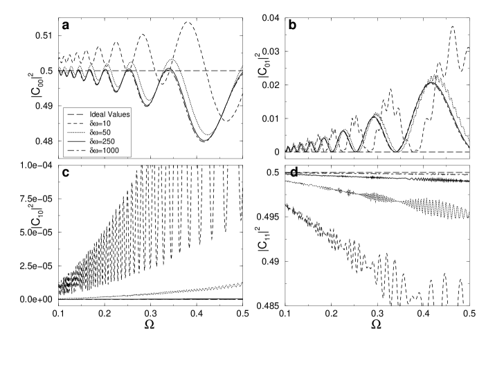
Figure 1: Dependence of final $\mathsf{CN}_{10}$-gate probabilities, $|C_{kl}|^{2}$ on the Rabi frequency, $\Omega$, for different values of $\delta\omega$. The values of $\Omega$ and $\delta\omega$ are given in units of $J$. (a) $|C_{00}|^{2}$. (b) $|C_{01}|^{2}$. (c) $|C_{10}|^{2}$. (d) $|C_{11}|^{2}$.

The simulated final probabilities are plotted in Fig. 1 as functions of the Rabi frequency for four different values of $\delta\omega$. All parameters in the simulation are given in units of $J$. We chose $\omega_{0}=100$. One can see that the variation of the probabilities definitely shows a dependence on $\delta\omega$ as well as an oscillatory dependence on the Rabi frequency. These dependencies can be explained by dividing the non-resonant transitions into two categories:

• Near-Resonant Transitions. In this case there is only one such transition, namely $|00\rangle_{l}\leftrightarrow|01\rangle_{l}$ which, for $\delta\omega=50$, has a transition frequency of $\nu=E_{1}-E_{0}=99.98$ as compared to $\nu=E_{3}-E_{2}=98.98$ for the resonant transition.

• Off-Resonant Transitions. In this case there are two, $|00\rangle_{l}\leftrightarrow|10\rangle_{l}$ and $|01\rangle_{l}\leftrightarrow|11\rangle_{l}$ which, for $\delta\omega=50$, have transition frequencies of 151.02 and 149.02 respectively.

The effects of all of the above transitions can clearly be seen in the $\delta\omega=10$ case. In Fig. 1(b), which shows the final values of $|C_{01}|^{2}$, the large amplitude low frequency oscillations are the result of the near-resonant transitions and the small amplitude high frequency oscillations are the result of the off-resonant transitions. In Fig. 1(c) for $|C_{10}|^{2}$, the primary effect is that of the high frequency oscillations since this state is not directly affected by the near-resonant transition, rather it is affected by an off-resonant one. Figure 1(d) for $|C_{11}|^{2}$ again shows the high frequency oscillations. However, the oscillations are modulated and shifted by the near-resonant transition. This may be explained by a two-step process, $|11\rangle_{l}\rightarrow|01\rangle_{l}\rightarrow|00\rangle_{l}$, an off-resonant transition followed by a near-resonant one. In Fig. 1(a) for $|C_{00}|^{2}$ the probability is primarily influenced by the near-resonant transition, but it is shifted upwards due to the off-resonant ones.

In order to decrease the errors on the $\mathsf{CN}_{10}$, one can reduce the Rabi frequency, which reduces the effect of all non-resonant transitions. Another method of error reduction can be explained by an analysis of Fig. 1. The graphs clearly show that increasing $\delta\omega$ decreases the influence of the off-resonant transitions. This is due to the fact that it increases the difference between the frequencies of the off-resonant transitions on the one hand, and that of the resonant one on the other. When $\delta\omega$ is 250, the effect of the off-resonant transitions is almost negligible.

The remaining error is due to the near-resonant transition. This error can be reduced by making use of the “$2\pi k$-method” 2 ; c , which essentially involves choosing values of the Rabi frequency where the error due to the near-resonant transition is zero. That is, a Rabi frequency is chosen such that a $\pi$-pulse, while giving rise to the resonant transition will also cause an angular change of $2\pi k$ (where $k$ is an integer), due to the near-resonant one; so that the probabilities of the states affected by the near-resonant transition return to their initial values at the end of the pulse. The condition for this is,

$$\sqrt{\Omega_{0}^{2}+\Delta^{2}}\,\tau=2\pi k,$$ (18)

where $\tau=\pi/\Omega_{1}$ as before, and $\Delta$ is the difference between the near-resonant and resonant transition frequencies. Thus, for $\delta\omega\gtrsim 250$, the errors can effectively be reduced by choosing values for the Rabi frequency satisfying the $2\pi k$ condition. (Here, we don’t consider more sophisticated pulse shaping methods, which can also be used to reduce the errors in the implementation of quantum logic gates e ).

VI Shor’s Algorithm

Figure 2: (a) Probabilities of the logical states, $|C_{n}|^{2}$, following the 41-pulse sequence for Shor’s algorithm. The values of the parameters used in our simulations were, $J=30$, $\omega_{0}=100$, $\delta\omega=30$, $\Omega=0.5$. The white bars indicate ideal output probabilities of Shor’s algorithm, and the black bars are the results of our simulation. (b) The same probabilities, on an enlarged scale, to show the probabilities of unwanted logical states.

In order to illustrate the implementation of a quantum algorithm in our system, we have performed a simulation of Shor’s algorithm for prime factorizationd . We simulated a pulse sequence for the factorization of the number four in a four-spin Heisenberg chain quantum computer. This is a 16 level-system and the logical states are $|0000\rangle_{l},\ |0001\rangle_{l},\ |0010\rangle_{l},\ \dots\ |1111\rangle_{l}$, or in decimal notation $|0\rangle_{l},\ |1\rangle_{l},\ |2\rangle_{l},\ \dots\ |15\rangle_{l}$. We used the same sequence of quantum gates as the simulations on the Ising chain quantum computer c , but the pulses used were those appropriate to the Heisenberg case.

Shor’s algorithm requires two registers of qubits. We designate the left two logical qubits as the x-register and the right as the y-register. We assume that the initial state is the ground state $|0000\rangle_{l}=|0\rangle_{l}$. The algorithm then proceeds in three steps. The first step is to create a uniform superposition in the logical x-register. The state which results from this is,

$$|\Psi\rangle = {1\over 2}\,(|0000\rangle_{l}+|0100\rangle_{l}+|1000\rangle_{l}+|1100\rangle_{l})$$ (19)

$$\equiv {1\over 2}\,(|0\rangle_{l}+|4\rangle_{l}+|8\rangle_{l}+|12\rangle_{l}),$$

The resonant pulse sequence to create this state consists of three $\pi/2$-pulses - for the transitions $|0\rangle_{l}\leftrightarrow|4\rangle_{l}$, then $|0\rangle_{l}\leftrightarrow|8\rangle_{l}$, then $|4\rangle_{l}\leftrightarrow|12\rangle_{l}$. The next step is to transform to the state,

$$|\Psi\rangle={1\over 2}\sum_{x=0}^{3}|x,\,y(x)\rangle_{l},$$ (20)

where $y(x)=3^{x}$(mod 4). This is implemented using six $\pi$-pulses. The final step is to perform a discrete Fourier transform on the logical x-register. This can be implemented using a sequence of so-called $\mathsf{A}$- and $\mathsf{B}$-gates, which in our system requires 32 ($\pi$- and $\pi/2$-) pulses. The final state after implementation of Shor’s algorithm ideally contains the following four states with equal probability,

$$|0001\rangle_{l},\qquad|0011\rangle_{l},\qquad|0101\rangle_{l},\qquad\textrm{and}\qquad|0111\rangle_{l},$$

or,

$$|1\rangle_{l},\qquad|3\rangle_{l},\qquad|5\rangle_{l},\qquad\textrm{and}\qquad|7\rangle_{l}.$$ (21)

Figure 2 shows the results of our numerical simulations of the 41-pulse sequence. The white bars correspond to the ideal values of the probabilities (1/4) of the states in (21). The black bars are the probabilities resulting from numerical simulations of the pulse sequence. The larger probabilities are shown in Fig. 2(a), and the smaller ones corresponding to errors are shown on an enlarged scale in Fig. 2(b). It can be seen that the simulated probabilities for the states in (21) are very close to their ideal values. The maximum deviation on these states is 0.0066. The probabilities of the unwanted states do not exceed 0.0043. Four unwanted states have probabilities between 0.0030 and 0.0043, and the remainder have probabilities smaller than 0.0005. The sum of the probabilities of the unwanted states is 0.016.

VII Conclusions

We have demonstrated a scheme for the implementation of quantum information processing in a system of particles with strong permanent interactions. We envisage that a number of these systems could be used for the design of quantum logical devices. We have also shown that a system of strongly coupled particles is qubitless - logical qubits don’t directly correspond to any physical two-state subsystem. Nevertheless, it is possible to implement quantum logic operations in this system.

As an example, we presented results on the implementation of the controlled-NOT gate and Shor’s algorithm in a spin-1/2 Heisenberg chain in a nonuniform magnetic field. The results show that quantum logic can be implemented with resonant electromagnetic pulses and that the errors caused by nonresonant transitions can be effectively reduced.

- (1) C. Williams, S. Clearwater, Explorations in Quantum Computing, (Springer-Verlag, Berlin, 1995).
- (2) G.P. Berman, G.D. Doolen, R. Mainieri, V.I. Tsifrinovich, Introduction to Quantum Computers, (World Scientific, Singapore, 1998).
- (3) Introduction to Quantum Computation and Information, edited by H. K. Lo, S.Popescu, T. Spiller, (World Scientific, Singapore, 1998).
- (4) D.P. DiVincenzo, D. Bacon, J. Kempe, G. Burkard, K.B. Whaley, Nature, 408, 339 (2000).
- (5) A. Barenco, C.H. Bennett, R. Cleve, D. P. DiVincenzo, N. Margolus, P. Shor, T. Sleator, J. Smolin, H. Weinfurter, Phys. Rev. A, 52, 3457 (1995).
- (6) G.P. Berman, G.D. Doolen, G.V. López, V.I. Tsifrinovich, Phys. Rev. A, 61, 042307-1 (2000).
- (7) G.D. Sanders, K.W. Kim, W.C. Holton, Phys. Rev. A, 59, 1098 (1999).
- (8) P. Shor, in Proc. 35th Annual Symposium on the Foundations of Computer Science, (IEEE Computer Society Press, New York, 1994), p. 124.