Quantum contact interactions

Abstract

The existence of several exotic phenomena, such as duality and spectral anholonomy is pointed out in one-dimensional quantum wire with a single defect. The topological structure in the spectral space which is behind these phenomena is identified.

1. Introduction

Since the successful applications of the quantum field theories to the high energy particle physics, the low-energy phenomena described by the non-relativistic quantum mechanics has been regarded, in a way, as an area of rear guard action. With the advent of quantum information theory, however, it is recognized that a seemingly simple system in elementary quantum mechanical setting can have highly nontrivial properties with potential technological ramifications.

In this article, we point out a different kind of nontriviality of generic low energy quantum mechanics other than that related to the entanglement. The key concept here is the contact, or point interaction. Let us suppose that we have a one-dimensional quantum particle subjected to a potential of finite support. If the range of the potential is small enough compared to the wave length of the particle, one should be able to approximate the action of the potential as operating at a single location. In other word, one can regard the system as being free everywhere except the vicinity of of a single point. Every student of elementary quantum mechanics learns that such system is described by a singular object called Dirac’s $\delta$-function potential, which induces the discontinuity of the space derivative of the wave functions. However, a natural question might arise to every naive mind: Why is the discontinuity allowed only for the derivative, not the wave function itself? The answer to this question is not to be found in any elementary textbooks. Indeed, it turns out that there is no good reason to reject the discontinuity of the wave function itself. We shall see in the followings that this possibility opens up a whole new vista to the problem.

2. Generalized point interaction described by U(2)

We place a quantum particle on a one-dimensional line with a defect located at $x=0$. In formal language, the system is described by the Hamiltonian

$$H=-{{1}\over{2}}{{d^{2}}\over{dx^{2}}},$$ (1)

defined on proper domains in the Hilbert space ${\cal H}=L^{2}({\bf R}\setminus\{0\})$. We ask what the most general condition at $x=0$ is. We define the two-component vectors  [?],

$$\Phi=\left({\matrix{{\varphi(0_{+})}\cr{\varphi(0_{-})}\cr}}\right)\ \ \ {\rm and}\ \ \ \Phi^{\prime}=\left({\matrix{{\varphi^{\prime}(0_{+})}\cr{-\varphi^{\prime}(0_{-})}\cr}}\right)$$ (2)

from the values and derivatives of a wave function $\varphi(x)$ at the left $x=0_{-}$ and the right $x=0_{+}$ of the missing point. The requirement of self-adjointness of the Hamiltonian operator (1) is satisfied if probability current $j(x)=-i((\varphi^{*})^{\prime}\varphi-\varphi^{*}\varphi^{\prime})/2$ is continuous at $x=0$. In terms of $\Phi$ and $\Phi^{\prime}$, this requirement is expressed as

$$\Phi^{\prime\dagger}\Phi-\Phi^{\dagger}\Phi^{\prime}=0,$$ (3)

which is equivalent to $|\Phi-iL_{0}\Phi^{\prime}|$ $=$ $|\Phi+iL_{0}\Phi^{\prime}|$ with $L_{0}$ being an arbitrary constant in the unit of length. This means that, with a two-by-two unitary matrix $U\in U(2)$, we have the relation,

$$(U-I)\Phi+iL_{0}(U+I)\Phi^{\prime}=0\ .$$ (4)

This shows that the entire family $\Omega$ of contact interactions admitted in quantum mechanics is given by the group $U(2)$. A standard parametrization for $U\in U(2)$ is

$$U=e^{i\xi}\left({\matrix{{\alpha}&{\beta}\cr{-\beta^{*}}&{\alpha^{*}}\cr}}\right),\ \ \ \xi\in[0,\pi),\ \ \ \alpha,\beta\in{\bf C};\ \ |\alpha|^{2}+|\beta|^{2}=1.$$ (5)

In mathematical term, the domain in which the Hamiltonian $H$ becomes self-adjoint is parametrized by $U(2)$ — there is a one-to-one correspondence between a physically distinct contact interaction and a self-adjoint Hamiltonian  [?]. We use the notation $H_{U}$ for the Hamiltonian with the contact interaction specified by $U\in\Omega$ $\simeq U(2)$.

If one asume $\Re\beta\neq 0$ and $\Im\beta\neq 0$, one can easily show that (2), (4), (5) is rearranged in the form

$$\left({\matrix{{\varphi(0_{+})}\cr{\varphi^{\prime}(0_{+})}\cr}}\right)=\Lambda\left({\matrix{{\varphi(0_{-})}\cr{\varphi^{\prime}(0_{-})}\cr}}\right),$$ (6)

with the form

$$\Lambda=e^{i\lambda}\left({\matrix{{s}&{u}\cr{v}&{t}\cr}}\right),\ \ \ \lambda\in[0,\pi),\ \ \ s,t,u,v\in{\bf R};\ st-uv=1.$$ (7)

This is the transfer matrix representation  [?], which has been the treated as the standard form of generalized point interaction. But it is now obvious that, unlike the $U(2)$ representation, (5), the form (7) does not cover the whole family of generalized point interaction, thus does not gives complete parametrization.

3. Fermion-boson duality

The transfer matrix form (7) is non-the-less useful in making contact with our intuition to the point interaction. If we set $s=t=1$, $uv=0$ has to be satisfied. By further choosing $\lambda=0$, one obtain two sets of one parameter family of transfer matrices

$$\Lambda_{\delta}(v)=\left(\begin{array}[]{cc}1&0\\ v&1\end{array}\right),\ \ \ \Lambda_{\varepsilon}(u)=\left(\begin{array}[]{cc}1&u\\ 0&1\end{array}\right).$$ (12)

The first one keeps the wave functions at $x=0_{+}$ and $0_{-}$ the same, while giving the jump at $x=0$ for the value of their derivatives: This clearly corresponds to the $\delta$ potential of strength $v$. The second one gives the jump in the wave function itself at the location of the defect $x=0$. We call this contact interaction as $\varepsilon$ potential with the strength $u$. It can be proven with elementary algebra that this set of connection conditions is realizable as a singular zero-range limit of three-peaked structure  [?,?]. It is anticipated from the construction that $\delta$ and $\varepsilon$ potentials play a complimentary role. An evident is that $\delta$ interaction at the origin has no effect on odd-parity states, while $\varepsilon$ has no effect on even-parity states. A more quantitative expression of the complimentarity is obtained by considering the scattering properties of the $\delta$ and $\varepsilon$ potentials. We start by putting a generalized contact interaction at the origin on $x$-axis. Incident and outgoing waves can be written as

$$\varphi_{in}(x) = A(k)e^{ikx}+B(k)e^{-ikx}\ \ \ (x<0),$$ (13)

$$\varphi_{out}(x) = e^{ikx}\ \ \ \ \ \ \ \ \ \ \ \ \ \ \ \ \ \ \ \ \ \ \ \ \ \ \ \ \ \ \ \ \ \ (x>0).$$ (14)

The connection condition (6) is written as

$$\left(\!\!\begin{array}[]{c}1\\ ik\end{array}\!\!\right)=\Lambda\left(\begin{array}[]{cc}1&1\\ ik&-ik\end{array}\right)\left(\!\!\begin{array}[]{c}A(k)\\ B(k)\end{array}\!\!\right).$$ (21)

The transmission and reflection coefficients are calculated respectively as

$$T(k)=\left|\frac{1}{A(k)}\right|^{2},\hskip 21.52771ptR(k)=\left|\frac{B(k)}{A(k)}\right|^{2}.$$ (22)

In case of $\Lambda=\Lambda_{\delta}(v)$, we obtain the well-known results

$$T_{\delta}(k)=\frac{k^{2}}{k^{2}+(v/2)^{2}},\hskip 8.61108ptR_{\delta}(k)=\frac{(v/2)^{2}}{k^{2}+(v/2)^{2}}.$$ (23)

For $\Lambda=\Lambda_{\varepsilon}(u)$, we obtain

$$T_{\varepsilon}(k)=\frac{(2/u)^{2}}{k^{2}+(2/u)^{2}},\hskip 8.61108ptR_{\varepsilon}(k)=\frac{k^{2}}{k^{2}+(2/u)^{2}}.$$ (24)

One can observe that if $u=v$, $T_{\delta}(k)=T_{\varepsilon}(1/k)$ and $R_{\delta}(k)=R_{\varepsilon}(1/k)$ are satisfied. This implies that the low (high) energy dynamics of $\varepsilon$ potential is described by the high (low) energy dynamics of $\delta$ potential.

The dual role of $\delta$ and $\varepsilon$ potentials becomes more manifest when we consider the scattering of two identical particles. We now regard the variable $x$ as the relative coordinate of two identical particles whose statistics is either fermionic or bosonic. The incoming and outgoing waves are now related by the exchange symmetry. We assume the form

$$\varphi_{in}(x) = e^{ikx}+C(k)e^{-ikx}\ \ \ \ \ \ \ \ \ \ \ \ \ (x<0),$$ (25)

$$\varphi_{out}(x) = \pm e^{-ikx}\pm C(k)e^{ikx}\ \ \ \ \ \ \ \ \ \ (x>0).$$ (26)

where the composite signs take $+$ for bosons and $-$ for fermions. Important fact to note is that the symmetry (anisymmetry) of $\varphi(x)$ leads to the antisymmetry (symmetry) of it’s derivative $\varphi^{\prime}(x)$. The coefficient $C(k)$ becomes the scattering matrix. The connection condition in (6) now reads

$$\left[\left(\begin{array}[]{cc}1&1\\ -ik&ik\end{array}\right)\mp\Lambda\left(\begin{array}[]{cc}1&1\\ ik&-ik\end{array}\right)\right]\left(\!\!\begin{array}[]{c}C(k)\\ 1\end{array}\!\!\right)=0.$$ (33)

We first consider the case for $\delta$ potential $\Lambda$ $=\Lambda_{\delta}(v)$. We obtain

$$C_{\delta}(k) = 1\ \ \ \ \ \ \ \ \ \ \ \ \ \ \ \ \ {\rm for\ fermions},$$ (34)

$$C_{\delta}(k) = {{2ik+v}\over{2ik-v}}\ \ \ \ \ {\rm for\ bosons}.$$ (35)

The first equation means that the $\delta$ function is inoperative as the two-body interaction between identical bosons, which is an obvious fact pointed out earlier. Next we consider the case of $\varepsilon$ potential $\Lambda$ $=\Lambda_{\varepsilon}(u)$. We have

$$C_{\varepsilon}(k) = {{2ik+4/u}\over{2ik-4/u}}\ \ \ {\rm for\ fermions},$$ (36)

$$C_{\varepsilon}(k) = 1\ \ \ \ \ \ \ \ \ \ \ \ \ \ \ \ \ \ {\rm for\ bosons}.$$ (37)

One finds that the role of fermion and boson cases are exchanged: The $\varepsilon$ potential as the two-body interaction has no effect on identical bosons, but does have an effect on the fermions. Moreover, the scattering amplitude of fermions with $\Lambda_{\varepsilon}(u)$ is exactly the same as that of bosons with $\Lambda_{\delta}(v)$ if the two coupling constants are related as

$$vu=4.$$ (38)

Therefore, a two-fermion system with $\varepsilon$ potential is dual to a two-boson system with $\delta$ potential with role of the strong and week coupling reversed. As expected, a natural generalization to $N$-particle systems exists  [?].

4. Spectral space decomposition and spiral anholonomy

We now go back to the general $U(2)$ representation of the contact interaction, and look at the structure of the parameter space more closely. Let us consider following generalized parity transformations  [?,?]:

$${\cal P}_{1} : \varphi(x)\longrightarrow({\cal P}_{1}\varphi)(x)=\varphi(-x),$$ (39)

$${\cal P}_{2} : \varphi(x)\longrightarrow({\cal P}_{2}\varphi)(x)=i[\Theta(-x)-\Theta(x)]\varphi(-x)\ ,$$ (40)

$${\cal P}_{3} : \varphi(x)\longrightarrow({\cal P}_{3}\varphi)(x)=[\Theta(x)-\Theta(-x)]\varphi(x)\ .$$ (41)

These transformations satisfy the anti-commutation relation

$${\cal P}_{i}{\cal P}_{j}=\delta_{ij}+i\epsilon_{ijk}{\cal P}_{k}.$$ (42)

Since the effect of ${\cal P}_{i}$ on the boundary vectors $\Phi$ and $\Phi^{\prime}$ are given by $\Phi\buildrel{\cal P}_{i}\over{\longrightarrow}\sigma_{i}\Phi\ ,$ $\Phi^{\prime}\buildrel{\cal P}_{i}\over{\longrightarrow}\sigma_{i}\Phi^{\prime}\ ,$ where $\{\sigma_{i}\}$ are the Pauli matrices, the transformation ${\cal P}_{i}$ on an element $H_{U}$$\in\Omega$ induces the unitary transformation

$$U\buildrel{\cal P}_{i}\over{\longrightarrow}\sigma_{i}U\sigma_{i}$$ (43)

on an element $U$ $\in$ $U(2)$. The crucial fact is that the transformation ${\cal P}_{i}$ turns one system belonging to $\Omega$ into another one with same spectrum. In fact, with any ${\cal P}$ defined by

$${\cal P}=\sum_{j=1}^{3}c_{j}\,{\cal P}_{j}$$ (44)

with real $c_{j}$ with constraint $\sum_{j=1}^{3}c_{j}^{2}=1$, one has a transformation

$${\cal P}H_{U}{\cal P}=H_{U_{\cal P}}$$ (45)

where $U_{\cal P}$ is given by

$$U_{\cal P}=\sigma U\sigma\ \ \ {\rm with}\ \ \ \sigma=\sum_{j=1}^{3}c_{j}\,\sigma_{j}.$$ (46)

One sees, from (45), that the system described by the Hamiltonians $H_{U}$ has a family of systems $H_{U_{\cal P}}$ which share the same spectrum with $H_{U}$.

Let us suppose that the matrix $U$ is diagonalized with appropriate $V\in SU(2)$ as

$$U=V^{-1}DV.$$ (47)

With the explicit representations

$$D=e^{i\xi}e^{i\rho\sigma_{3}}=\left({\matrix{{e^{i\theta_{+}}}&0\cr 0&{e^{i\theta_{-}}}\cr}}\right),\ \ \ \ \theta_{\pm}=\xi\pm\rho,$$ (48)

and

$$V=e^{i{\mu\over 2}\sigma_{2}}e^{i{\nu\over 2}\sigma_{3}},$$ (49)

one can show easily that with $\sigma_{V}$ $=$ $e^{-i{\nu\over 2}\sigma_{3}}$ $e^{-i{\mu\over 2}\sigma_{2}}$ $e^{i{\nu\over 2}\sigma_{3}}\sigma_{3}$ $=\sigma_{V}^{-1}$, one has

$$U=\sigma_{V}D\sigma_{V}$$ (50)

which is of the type (46). This means that $H_{U}$ and $H_{D}$ share the same spectra. One can therefore conclude that the spectrum of the system described by $H_{U}$ is uniquely determined by the eigenvalue of $U$, and also that a point interaction characterized by $U$ possesses the isospectral subfamily

$$\Omega_{iso}=\left\{H_{V^{-1}DV}|V\in SU(2)\right\},$$ (51)

which is homeomorphic to the 2-sphere specified by the polar angles $(\mu,\nu)$.

$$\Omega_{iso}=\left\{(\mu,\nu)|\mu\in[0,\pi],\nu\in[0,2\pi)\right\}\simeq S^{2}.$$ (52)

There is of course an obvious exception to this for the case of $D$ $\propto I$, in which case, $\Omega_{iso}$ consists only of $D$ itself.

To see the structure of the spectral space, i.e. the part of parameter space $U(2)$ that determines the distinct spectrum of the system, it is convenient to make the spectrum of the system discrete. Here, for simplicity, we consider the line $x\in[-l,l]$ with Dirichlet boundary, $\varphi(-l)$ $=\varphi(l)$ $=0$. Then, the wave function is of the form

$$\varphi(x) = A_{+}\sin{k(x-l)}\ \ \ \ \ \ \ (x>0)$$ (53)

$$= A_{-}\sin{k(x+l)}\ \ \ \ \ \ \ (x<0).$$ (54)

One then has

$$\left({\matrix{{\varphi(0_{+})}\cr{\varphi(0_{-})}\cr}}\right) = \sin{kl}\Phi_{0},$$ (55)

$$\left({\matrix{{\varphi^{\prime}(0_{+})}\cr{-\varphi^{\prime}(0_{-})}\cr}}\right) = k\cos{kl}\Phi_{0},$$ (56)

with some common constant vector $\Phi_{0}$. Putting this form into the connection condition (4), we obtain

$$1+kL_{0}\cot{kl}\cot{\theta_{+}\over 2} = 0,$$ (57)

$$1+kL_{0}\cot{kl}\cot{\theta_{-}\over 2} = 0.$$ (58)

This means that the spectrum of the system is effectively split into that of two separate systems of same structure, each characterized by the parameters $\theta_{+}$ and $\theta_{-}$. So the spectra of the system is uniquely determined by two angular parameters $\{\theta_{+},\theta_{-}\}$.

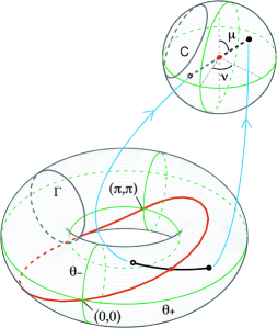
Figure  1.: The spectral torus $(\theta_{+},\theta_{-})$ and the isospectral sphere $(\mu,\nu)$.

The entire parameter space $\Omega$ = $\{\theta_{+},\theta_{-},\mu,\nu\}$ is a product of spectral space 2-torus

$$\Omega_{sp} = \left\{(\theta_{+},\theta_{-})|\theta_{+},\theta_{-}\in[0,2\pi]\right\}$$ (59)

$$\simeq T^{2}=S^{1}\times S^{1},$$ (60)

and the isospectral space $\Omega_{iso}$ = $\{\mu,\nu\}$ $\simeq S^{2}$ (See Fig. 1). There is another way to characterize this torus using a spin matrix

$$\sigma_{S}=\sigma_{V}\sigma_{3}\sigma_{V}.$$ (61)

Clearly, one has

$$\sigma_{S}U\sigma_{S}=U,$$ (62)

which means that the torus $\Omega_{sp}$ is the submanifold of $\Omega$ that is invariant with the symmetry operation related to $\sigma_{S}$.

There is one more subtle point missing in the foregoing argument: We note that this parameter space provides a double covering for the family of point inteactions $\Omega\simeq U(2)$ due to the arbitrariness in the interchange $\theta_{+}\leftrightarrow\theta_{-}$. Accordingly, two systems with interchanged values for $\theta_{+}$ and $\theta_{-}$ are isospectral. So the space of distinct spectra $\Sigma$ is the torus $T^{2}=\{(\theta_{+},\theta-)|\theta_{\pm}\in[0,2\pi)\}$ subject to the identification $(\theta_{+},\theta_{-})$ $\equiv(\theta_{-},\theta_{+})$. Thus we have

$$\Sigma=\{Spec(H_{U})|U\in\Omega\}=T^{2}/{\bf Z}_{2},$$ (63)

which is homeomorphic to a Möbius strip with boundary  [?].

Looking this double covering nature of the spectral torus from the other side, one may also say that on the isospectral $S^{2}$, the point interactions corresponding to the two polar opposite positions occupy a special positions, because they belong to the same spectral $T^{2}$ sharing the same symmetry invariance (62). We call these pairs dual to each other. One particular example is this duality is is given by $\{\mu=\pi/2,\nu=0\}$ and $\{\mu=\pi/2,\nu=\pi\}$. These pairs belong to the parity (in original left-right sense) invariant torus $\sigma_{1}U\sigma_{1}$ $=U$. One can check immediately that this essentially is the duality between the $\delta$ interaction system and $\varepsilon$ interaction system with opposite parity states which has appeared in the previous section.

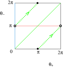
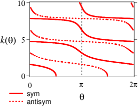
Figure  2.: Spiral anholonomy on the torus $\{\theta_{+}.\theta_{-}\}$.

An intriguing phenomenon is revealed by a closer examination of the spectral equation (57). Obviously, energy spectrum as a function of the parameter $\theta_{+}$ or $\theta_{-}$ has to be a $2\pi$-periodic function. With elementary calculation, however, one can explicitly see the relations

$${{dk\ }\over{d\theta_{+}}},\ \ {{dk\ }\over{d\theta_{-}}}<0.$$ (64)

The only way to reconcile these two facts is through the “spectral flow” ; namely, when $\theta_{\pm}$ is increased by $2\pi$, an energy eigenstate is shifted to a lower eigenstate while the spectra as a whole are unchanged  [?]. The situation becomes clear by the illustration shown in Fig. 2, where the spectra is plotted as functions of $\theta=$$\theta_{+}=$ $\theta_{-}+\pi/2$. The root of this phenomenon is the nontrivial topology of the spectral space $T^{2}$, as expressed in the homotopy group $\pi_{1}(T^{2})={\bf Z}\times{\bf Z}$. This type of “spiral anholonomy” has been known in quantum physics only in non-Abelian gauge theories until now.

At this point, some readers might be wondering whether nontrivial topology of the isospectral sphere, $\pi_{2}(S^{2})={\bf Z}$, has any observable consequences. We simply note that affirmative answers are given in the form of Berry phase  [?,?].

5. A Prospect

Immediate and useful extensions of our treatment exist for the quantum mechanics on the graphs  [?]. The analysis of so-called “X-junction” in terms of $U(4)$ parameter space appears to have particular urgency because of its potential relevance to the quantum informational devices  [?].

This work has been supported in part by the Monbu-Kagakusho Grant-in-Aid for Scientific Research (No. (C)13640413).

REFERENCES

- [1] T. Fülöp and I. Tsutsui Phys. Lett. A264, 366 (2000).
- [2] P. Šeba, Czech. J. Phys. B36, 667 (1986).
- [3] S. Albeverio, F. Gesztesy, R. Høegh-Krohn and H. Holden, Solvable Models in Quantum Mechanics (Springer, Heidelberg, 1988).
- [4] T. Cheon and T. Shigehara, Phys. Lett. A243, 111 (1998).
- [5] P. Exner, H. Neidhardt and A. Zagrebnov, Comm. Math. Phys. 224, 593 (2001).
- [6] T. Cheon and T. Shigehara, Phys. Rev. Lett. 82, 2539 (1999).
- [7] I. Tsutsui, T. Fülöp and T. Cheon, J. Phys. Soc. Jpn, 69, 3473 (2000).
- [8] T. Cheon, T. Fülöp and I. Tsutsui, Ann. of Phys. (NY) 294, 1 (2001).
- [9] I. Tsutsui, T. Fülöp and T. Cheon, J. Math. Phys. 42 5687 (2001).
- [10] T. Cheon, Phys. Lett. A248, 285 (1998).
- [11] T. Cheon and T. Shigehara, Phys. Rev. Lett. 76, 1770 (1996).
- [12] M. Brazovskaia and P. Pieranski, Phys. Rev. E58, 4076 (1998).
- [13] P. Exner, Lett. Math. Phys. 38, 313 (1996); ibid. 42 193 (1997) .
- [14] S. Bose and D. Home, Phys. Rev. Lett. 88, 050401 (2002).