Quantum learning and universal quantum matching machine

Abstract

Suppose that three kinds of quantum systems are given in some unknown states $\left|f\right\rangle^{\otimes N}$, $\left|g_{1}\right\rangle^{\otimes K}$, and $\left|g_{2}\right\rangle^{\otimes K}$, and we want to decide which template state $\left|g_{1}\right\rangle$ or $\left|g_{2}\right\rangle$, each representing the feature of the pattern class ${\cal C}_{1}$ or ${\cal C}_{2}$, respectively, is closest to the input feature state $\left|f\right\rangle$. This is an extension of the pattern matching problem into the quantum domain. Assuming that these states are known a priori to belong to a certain parametric family of pure qubit systems, we derive two kinds of matching strategies. The first is a semiclassical strategy which is obtained by the natural extension of conventional matching strategies and consists of a two-stage procedure: identification (estimation) of the unknown template states to design the classifier (learning process to train the classifier) and classification of the input system into the appropriate pattern class based on the estimated results. The other is a fully quantum strategy without any intermediate measurement which we might call as the universal quantum matching machine. We present the Bayes optimal solutions for both strategies in the case of $K=1$, showing that there certainly exists a fully quantum matching procedure which is strictly superior to the straightforward semiclassical extension of the conventional matching strategy based on the learning process.

I Introduction

Distinguishing quantum systems is one of the central tasks in quantum information theory. We have a useful formalism known as quantum detection and estimation theory for dealing with this problem Helstrom_QDET ; Holevo_book ; PeresBook . Recent progress in quantum communication and computation provides motivations to generalize this theory and apply it to various new situations. Depending on our purposes there may be various scenaria in the problem of distinguishing quantum systems. The systems to be distinguished can be sometimes a set of given quantum states, and sometimes a set of possible quantum dynamics. These systems are usually generated by a quantum source which is expected to have certain characteristic features. If the source generates a completely random phenomena, then it is impossible to extract any meaningful information from it and therefore such a case will not come into our consideration. In a broad sense, we may then essentially have three possible circumstances:

• (1) the source identity, i. e. a set of possible quantum systems and associated probability distribution, is completely known;

• (2) the source identity is unknown, but it belongs to a parametrized family of quantum systems and probability distributions;

• (3) the source is known to be stationary and ergodic, but no other information is available.

The case $(1)$ has long been a main subject of quantum detection and estimation theory. However, the other two cases are becoming of practical importance in quantum information technology. Suppose, for example, we are interested in finding efficient representations of incoming random sequences of quantum states. If the source identity is completely known then we have well known theorems on the asymptotic average length of codewords and efficient coding algorithms are being developed and will be of practical use in the near future.

Consider then the situation in which the source identity is not completely known, which is indeed the case when dealing with a realistic quantum source. The obvious way to proceed would be by direct estimation of the source identity, which is then used in the coding algorithm in place of the unknown information of the source. When the source is known to be a member of a parametric family then the unknown parameters are readily estimated from the incoming training data. With enough data the estimate will be sufficiently close to the truth and the representation will be nearly optimal. On the other hand, if only a limited number of training data are available, one has to consider an appropriate estimation strategy which would hopefully be not only asymptotically optimal when the length of the training set tends to infinity, but be also optimal for intermediate amounts of training data. This kind of problem is known as learning strategy in conventional information theory, in particular in pattern matching theory Fu76 ; Fukunaga90 . Reasonable criteria which are usually assumed for a good strategy are:

• (i) no knowledge of the source is required;

• (ii) the delay due to the learning process is not long;

• (iii) the strategy should be simple and easy to implement.

The purpose of this paper is to develop a formalism for the quantum learning strategy and to apply it to the problem of distinguishing quantum systems in cases $(2)$ and $(3)$. In a recent paper Sasaki_Carlini_Jozsa2001a , the authors considered the problem of quantum pattern matching, in which each pattern class ${\cal C}_{i}$ is represented by a known quantum state $\left|g_{i}\right\rangle$ called a template state, and the task is to find a template which optimally matches a given unknown quantum state $\left|f\right\rangle$. Namely we have assumed that the input states $\left|f\right\rangle$ are given as quantum information (i.e. unknown quantum states) whereas the template states $\left|g_{i}\right\rangle$’s with known identities are given as classical information. Our goal was to obtain the best template as classical information (i.e. knowledge of the identity of the best $\left|g_{i}\right\rangle$) via a suitable matching strategy which is represented by a probability operator measure (POM), also referred to as a positive operator valued measure (POVM).

In the present paper we relax the ingredients of our previous formulation in the following way. That is, instead of fully knowing the identities of the template states we may be given only some finite number ($K$) of copies of each template (so our original formulation is equivalent to $K=\infty$). One matching strategy would then be to apply state estimation to the sets of $K$ copies and proceed as in our original formulation with the resulting estimated state identities. But this is unlikely to be an optimal strategy, since any intermediate measurement process generally degrades the classification performance, as shown in Ref. Sasaki_Carlini_Jozsa2001a . Following the criteria (i)$\sim$(iii), we should consider a more fully quantum procedure which, for any input $\left|f\right\rangle$, identifies the best template class without attempting to obtain any further information about the identities of the template states themselves.

Unfortunately, however, it seems still difficult to deal with this problem in general contexts. Therefore, we mainly consider here some tractable cases in order to illustrate how the quantum matching strategy should work in general. In particular, we assume that we a priori know that the input feature state $\left|f\right\rangle$ and the template states $\left|g_{1}\right\rangle$ and $\left|g_{2}\right\rangle$ belong to the following parametrized families of pure quantum states:

$$\left|f\right\rangle \equiv {1\over\sqrt{2}}\left(\left|\uparrow\right\rangle+{\rm e}^{if}\left|\downarrow\right\rangle\right),$$ (1)

$$\left|g_{1}\right\rangle \equiv {1\over\sqrt{2}}\Big{(}\left|\uparrow\right\rangle+{\rm e}^{ig_{1}}\left|\downarrow\right\rangle\Big{)},$$ (2)

$$\left|g_{2}\right\rangle \equiv {1\over\sqrt{2}}\Big{(}\left|\uparrow\right\rangle+{\rm e}^{ig_{2}}\left|\downarrow\right\rangle\Big{)},$$ (3)

where the parameters $f$, $g_{1}$, and $g_{2}$ are completely unknown. In this model, we will compare the semiclassical matching strategy which is obtained by a natural extension of the conventional matching strategy, and its fully quantum counterpart which we will identify as the universal quantum matching machine.

II Semiclassical Matching Machine

We are now given only some finite number ($K$) of identical samples of each template $\left|g_{i}\right\rangle$ which represent the features of a class ${\cal C}_{i}(=1,...,M)$, but whose state identities are completely unknown. The input state $\left|f\right\rangle$ is also given as an unknown quantum state and we have $N$ identical copies of $\left|f\right\rangle$. For simplicity we set $M=2$, i.e., we study the problem of binary classification. Thus we start with a system described by the state

$$\left|\Psi\right\rangle\equiv\left|f\right\rangle^{\otimes N}\otimes\left|g_{1}\right\rangle^{\otimes K}\otimes\left|g_{2}\right\rangle^{\otimes K}.$$ (4)

We first analyze a semiclassical strategy which is a natural extension of conventional matching strategies. That is, we first apply state estimation to the template states, design a classifier based on the results, and then apply this to measure and classify the input feature state. (see Fig. 1).

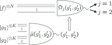
Figure 1: The semiclassical matching strategy. The POM $\{\hat{\mu}(g_{1}^{\prime},g_{2}^{\prime})\}$ is for estimating the unknown template states. The output $\{g_{1}^{\prime},g_{2}^{\prime}\}$ is used to design the classifier POM. In other words, using the training data $\hat{g}_{1}^{\otimes K}\otimes\hat{g}_{2}^{\otimes K}$, we fix the classifier to learn the appropriate template parameters.

This strategy is represented by two kinds of POMs; the first is for estimating the identities of the given unknown template states from the sets of $K$ samples $\hat{g}_{1}^{\otimes K}\otimes\hat{g}_{2}^{\otimes K}$ ($\hat{g}_{i}$ is understood as $\left|g_{i}\right\rangle\left\langle g_{i}\right|$). This POM is indexed by the possible outcomes $\{g_{1}^{\prime},g_{2}^{\prime}\}$ about the template identities and is denoted by $\{\hat{\mu}(g_{1}^{\prime},g_{2}^{\prime})\}$. The other is for classifying the input feature state with $N$ samples $\hat{f}^{\otimes N}$. This POM consists of two elements $\{\hat{\Omega}_{1}(g_{1}^{\prime},g_{2}^{\prime}),\hat{\Omega}_{2}(g_{1}^{\prime},g_{2}^{\prime})\}$ and should be the optimal matching strategy for the estimated templates $\{\hat{g}_{1}^{\prime},\hat{g}_{2}^{\prime}\}$, which was already given in our previous paper Sasaki_Carlini_Jozsa2001a . In this way each classifier POM element depends on the estimated parameters $\{g_{1}^{\prime},g_{2}^{\prime}\}$.

The problem here is then to find the optimal estimation strategy $\{\hat{\mu}(g_{1}^{\prime},g_{2}^{\prime})\}$. Such a strategy should maximize the following average score:

$$\bar{S}^{\mathrm{SC}}\equiv\sum_{(g_{1}^{\prime},g_{2}^{\prime})}\sum_{j=1}^{2}\left({1\over{2\pi}}\right)^{3}\int\int\int_{0}^{2\pi}dg_{1}dg_{2}df{\rm\,Tr}\,\left[\hat{\Omega}_{j}(g_{1}^{\prime},g_{2}^{\prime})\hat{f}^{\otimes N}\right]{\rm\,Tr}\,\left[\hat{\mu}(g_{1}^{\prime},g_{2}^{\prime})\hat{g}_{1}^{\otimes K}\otimes\hat{g}_{2}^{\otimes K}\right]\times|\langle f|g_{j}\rangle|^{2}.$$ (5)

The second trace-term in Eq. (5) is the conditional probability of having the outcomes $\{g_{1}^{\prime},g_{2}^{\prime}\}$ for the template states $\{\hat{g}_{1}^{\otimes K},\hat{g}_{2}^{\otimes K}\}$. The first trace-term is then the conditional probability that the input state $\hat{f}$ is classified into the $j$-th class when an appropriate matching strategy is applied to the $N$ identical input samples $\hat{f}^{\otimes N}$, and $|\langle f|g_{j}\rangle|^{2}$ is the conditional score.

Using the conventional terminology of pattern matching theory, the POM $\{\hat{\mu}(g_{1}^{\prime},g_{2}^{\prime})\}$ corresponds to the learning process to train the classifier $\{\hat{\Omega}_{j}(g_{1}^{\prime},g_{2}^{\prime})\}$ with given training samples $\{\hat{g}_{1}^{\otimes K},\hat{g}_{2}^{\otimes K}\}$. A well known method is the adaptive learning algorithm in which one first measures each pair of the training samples $\{\hat{g}_{1},\hat{g}_{2}\}$ and then updates the classifier parameters step by step for $K$ iterations under some appropriate updating rules. In contrast, the optimal learning strategy is expected to be a POM $\{\hat{\mu}(g_{1}^{\prime},g_{2}^{\prime})\}$ acting collectively on the state $\hat{g}_{1}^{\otimes K}\otimes\hat{g}_{2}^{\otimes K}$, i.e., fully exploiting the power of quantum entanglement.

The main purpose of this section is to develop a Bayesian formulation for the optimal learning strategy. First we introduce the score operators

$$\hat{W}(g_{j})\equiv{1\over{2\pi}}\int_{0}^{2\pi}df\hat{f}^{\otimes N}|\langle f|g_{j}\rangle|^{2},$$ (6)

just as in our previous paper, and rewrite Eq. (5) as

$$\bar{S}^{\mathrm{SC}}=\sum_{(g_{1}^{\prime},g_{2}^{\prime})}\left({1\over{2\pi}}\right)^{2}\int\int_{0}^{2\pi}dg_{1}dg_{2}{{\rm\,Tr}\,}\left[\hat{\mu}(g_{1}^{\prime},g_{2}^{\prime})\hat{g}_{1}^{\otimes K}\otimes\hat{g}_{2}^{\otimes K}\right]\sum_{j=1}^{2}{{\rm\,Tr}\,}\left[\hat{\Omega}_{j}(g_{1}^{\prime},g_{2}^{\prime})\hat{W}(g_{j})\right].$$ (7)

We then further introduce a learning score operator

$$\hat{G}(g_{1}^{\prime},g_{2}^{\prime})\equiv\left({1\over{2\pi}}\right)^{2}\int\int_{0}^{2\pi}dg_{1}dg_{2}\hat{g}_{1}^{\otimes K}\otimes\hat{g}_{2}^{\otimes K}\sum_{j=1}^{2}{{\rm\,Tr}\,}\left[\hat{\Omega}_{j}(g_{1}^{\prime},g_{2}^{\prime})\hat{W}(g_{j})\right],$$ (8)

and rewrite Eq. (7) as

$$\bar{S}^{\mathrm{SC}}=\sum_{(g_{1}^{\prime},g_{2}^{\prime})}{{\rm\,Tr}\,}\left[\hat{\mu}(g_{1}^{\prime},g_{2}^{\prime})\hat{G}(g_{1}^{\prime},g_{2}^{\prime})\right].$$ (9)

Thus the problem of finding the optimal learning strategy reduces to the estimation problem of the classifier parameters $g_{1}^{\prime}$ and $g_{2}^{\prime}$ through the learning score operator $\hat{G}(g_{1}^{\prime},g_{2}^{\prime})$.

Let us now proceed with the explicit calculation. We first need to evaluate $\sum_{j=1}^{2}{{\rm\,Tr}\,}\left[\hat{\Omega}_{j}(g_{1}^{\prime},g_{2}^{\prime})\hat{W}(g_{j})\right]$. If the score operator $\hat{W}(g_{j})$ were replaced by $\hat{W}(g_{j}^{\prime})$, then this quantity would be nothing but the average score appearing in the quantum template matching problem discussed in our previous paper Sasaki_Carlini_Jozsa2001a . In our previous work, the set $\{\hat{\Omega}_{1},\hat{\Omega}_{2}\}$ was designed for the a priori known parameters $g_{1}$ and $g_{2}$ of the template states. On the other hand, the POM $\{\hat{\Omega}_{1}(g_{1}^{\prime},g_{2}^{\prime}),\hat{\Omega}_{2}(g_{1}^{\prime},g_{2}^{\prime})\}$ here should be designed for the estimated parameters $\{g_{1}^{\prime},g_{2}^{\prime}\}$, while the score operators correspond to the unknown template states $\hat{g}_{1}$ or $\hat{g}_{2}$.

By definition, the POM $\{\hat{\Omega}_{1}(g_{1}^{\prime},g_{2}^{\prime}),\hat{\Omega}_{2}(g_{1}^{\prime},g_{2}^{\prime})\}$ should maximize the average score for $\hat{W}(g_{j}^{\prime})$ instead of $\hat{W}(g_{j})$, i.e. we should maximiize

$$\bar{S}^{\prime}=\sum_{j=1}^{2}{{\rm\,Tr}\,}\left[\hat{W}(g_{j}^{\prime})\hat{\Omega}_{j}(g_{1}^{\prime},g_{2}^{\prime})\right]={1\over 2}+{{\rm\,Tr}\,}\left[\left(\hat{W}(g_{1}^{\prime})-\hat{W}(g_{2}^{\prime})\right)\hat{\Omega}_{1}(g_{1}^{\prime},g_{2}^{\prime})\right],$$ (10)

where the resolution of the identity $\hat{\Omega}_{1}(g_{1}^{\prime},g_{2}^{\prime})+\hat{\Omega}_{2}(g_{1}^{\prime},g_{2}^{\prime})=\hat{I}$ was used in the second equality. The score operator $\hat{\Omega}_{1}(g_{1}^{\prime},g_{2}^{\prime})$ should be then taken to maximize ${\rm\,Tr}\,{\left[\left(\hat{W}(g_{1}^{\prime})-\hat{W}(g_{2}^{\prime})\right)\hat{\Omega}(g_{1}^{\prime},g_{2}^{\prime})\right]}$, that is, it should be the projection onto the subspace corresponding to the positive eigenvalues of the operator $\hat{W}(g_{1}^{\prime})-\hat{W}(g_{2}^{\prime})$. The score operators are built from the tensor product of $N$ identical copies of the input system, $\left|f\right\rangle^{\otimes N}$, and they are most appropriately described on the $N+1$ dimensional totally symmetric bosonic subspace of ${\cal H}^{\otimes N}$, ${\cal H}_{B}$, where $\{\left|m\right\rangle\}$ is the occupation number basis for the $\downarrow$ component. The score operators can then be written in the form

$$\hat{W}(g_{j}^{\prime})={1\over{2^{N+1}}}\left[\sum_{m=0}^{N}2\left|m\right\rangle\left\langle m\right|+\sum_{m=0}^{N-1}\sqrt{\bigg{(}\begin{array}[]{c}N\cr m\end{array}\bigg{)}\bigg{(}\begin{array}[]{c}N\cr m+1\end{array}\bigg{)}}\left({\rm e}^{ig_{j}^{\prime}}|m+1\rangle\langle m|+{\rm e}^{-ig_{j}^{\prime}}|m\rangle\langle m+1|\right)\right].$$ (11)

Therefore

$$\hat{W}(g_{1}^{\prime})-\hat{W}(g_{2}^{\prime})={{{\sin}\theta}\over{2^{N+1}}}\sum_{m=0}^{N-1}\sqrt{\bigg{(}\begin{array}[]{c}N\cr m\end{array}\bigg{)}\bigg{(}\begin{array}[]{c}N\cr m+1\end{array}\bigg{)}}\left({\rm e}^{i(\Theta+\pi/2)}|m+1\rangle\langle m|+{\rm e}^{-i(\Theta+\pi/2)}|m\rangle\langle m+1|\right),$$ (12)

where we have introduced $\Theta\equiv{{g_{1}^{\prime}+g_{2}^{\prime}}\over 2}$ and $\theta\equiv{{g_{1}^{\prime}-g_{2}^{\prime}}\over 2}$. Eq. (12) can also be rewritten as

$$\Delta\hat{W}(\Theta+{\pi\over 2},\theta)\equiv\hat{W}(g_{1}^{\prime})-\hat{W}(g_{2}^{\prime})=\hat{V}(\Theta+{\pi\over 2})\Delta\hat{W}(0,\theta)\hat{V}^{\dagger}(\Theta+{\pi\over 2}),$$ (13)

where

$$\hat{V}(\Theta)\equiv\sum_{m=0}^{N}{\rm e}^{im\Theta}\left|m\right\rangle\left\langle m\right|,$$ (14)

and

$$\Delta\hat{W}(0,\theta)\equiv{{{\sin}\theta}\over{2^{N+1}}}\sum_{m=0}^{N-1}\sqrt{\bigg{(}\begin{array}[]{c}N\cr m\end{array}\bigg{)}\bigg{(}\begin{array}[]{c}N\cr m+1\end{array}\bigg{)}}\big{(}|m+1\rangle\langle m|+|m\rangle\langle m+1|\big{)}.$$ (15)

Let the spectral decomposition of $\Delta\hat{W}(0,\theta)$ be

$$\Delta\hat{W}(0,\theta)=\sum_{m=0}^{N}\lambda_{m}\left|\lambda_{m}\right\rangle\left\langle\lambda_{m}\right|,$$ (16)

and introduce the POM

$$\hat{\Lambda}_{1}=\sum_{\lambda_{m}\geq 0}\left|\lambda_{m}\right\rangle\left\langle\lambda_{m}\right|,\quad\hat{\Lambda}_{2}=\sum_{\lambda_{m}<0}\left|\lambda_{m}\right\rangle\left\langle\lambda_{m}\right|.$$ (17)

Note that the $\{\left|\lambda_{m}\right\rangle\}$, and hence the $\{\hat{\Lambda}_{j}\}$, do not depend on $\theta$ while the eigenvalues $\lambda_{m}$ are proportional to ${\sin}\theta$. The optimal strategy for maximizing $\bar{S}^{\prime}$ (Eq. (10)) is then expressed by the POM

$$\hat{\Omega}_{j}(g_{1}^{\prime},g_{2}^{\prime})\equiv\hat{\Omega}_{j}(\Theta)=\hat{V}(\Theta+{\pi\over 2})\hat{\Lambda}_{j}\hat{V}^{\dagger}(\Theta+{\pi\over 2}).$$ (18)

The parameter $\Theta$ represents the relative position of the pair of the estimated states $\hat{g}_{1}^{\prime}$ and $\hat{g}_{2}^{\prime}$ from the $\hat{\sigma}_{x}$-axis in the Bloch sphere. This is the only parameter needed to specify the classifier, that is, the one to be learned from the training samples $\{\hat{g}_{1}^{\otimes K},\hat{g}_{2}^{\otimes K}\}$. The angle $\theta$ between $\hat{g}_{1}^{\prime}$ and $\hat{g}_{2}^{\prime}$ in the Bloch sphere, on the other hand, is irrelevant for the design of the classifier. The state configuration is depicted in Fig. 2.

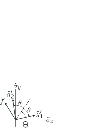
Figure 2: The configuration of the template states in the Bloch sphere representation. The input feature state and the template states lie on the great circle including the x and y axes in the Bloch sphere.

Using Eq. (18) we then obtain

$$\sum_{j=1}^{2}{{\rm\,Tr}\,}\left[\hat{\Omega}_{j}(g_{1}^{\prime},g_{2}^{\prime})\hat{W}(g_{j})\right] = \sum_{j=1}^{2}{{\rm\,Tr}\,}\left[\hat{\Omega}_{j}(\Theta)\hat{W}(g_{j})\right]$$ (19)

$$= {1\over 2}+{{\rm\,Tr}\,}\left[\hat{\Lambda}_{1}\Delta\hat{W}({{g_{1}+g_{2}}\over 2}-\Theta,{{g_{1}-g_{2}}\over 2})\right]$$

$$= {1\over 2}+\left[{\sin}(g_{1}-\Theta)-{\sin}(g_{2}-\Theta)\right]R_{N},$$

where

$$R_{N}\equiv{1\over{2^{N+1}}}\sum_{m=0}^{N-1}\sqrt{\bigg{(}\begin{array}[]{c}N\cr m\end{array}\bigg{)}\bigg{(}\begin{array}[]{c}N\cr m+1\end{array}\bigg{)}}\langle m|\hat{\Lambda}_{1}|m+1\rangle.$$ (20)

Therefore the learning score operator in Eq. (8) can be also rewritten as

$$\hat{G}(\Theta)=\left({1\over{2\pi}}\right)^{2}\int\int_{0}^{2\pi}dg_{1}dg_{2}\hat{g}_{1}^{\otimes K}\otimes\hat{g}_{2}^{\otimes K}\left\{{1\over 2}+\Bigl{[}{\sin}(g_{1}-\Theta)-{\sin}(g_{2}-\Theta)\Bigr{]}R_{N}\right\}.$$ (21)

Then the average score of Eq. (9) finally reads

$$\bar{S}^{\mathrm{SC}}=\sum_{\Theta}{{\rm\,Tr}\,}\left[\hat{\mu}(\Theta)\hat{G}(\Theta)\right].$$ (22)

After the integration of $g_{1}$ and $g_{2}$, the learning score operator $\hat{G}(\Theta)$ is represented by

$$\hat{G}(\Theta)={1\over 2}\hat{C}\otimes\hat{C}+{R_{N}\over 2}\left[\hat{D}(\Theta)\otimes\hat{C}-\hat{C}\otimes\hat{D}(\Theta)\right],$$ (23)

where

$$\hat{C} \equiv {1\over{2^{K}}}\sum_{k=0}^{K}\bigg{(}\begin{array}[]{c}K\cr k\end{array}\bigg{)}\left|k\right\rangle\left\langle k\right|,$$ (26)

$$\hat{D}(\Theta) \equiv \frac{i}{2^{K}}\sum_{k=0}^{K-1}\sqrt{\biggl{(}\begin{array}[]{c}K\cr k\end{array}\bigg{)}\bigg{(}\begin{array}[]{c}K\cr k+1\end{array}\biggr{)}}\Bigl{(}{\rm e}^{i\Theta}|k+1\rangle\langle k|-{\rm e}^{-i\Theta}|k\rangle\langle k+1|\Bigr{)}.$$ (31)

The basis $\{\left|k\right\rangle\}$ is the symmetric bosonic basis for the system of $K$ identical copies of the template states $\hat{g}_{1}^{K}$ or $\hat{g}_{2}^{K}$. Although we have not succeeded yet in deriving the optimal POM $\{\hat{\mu}(\Theta)\}$ maximizing the above score $\bar{S}$ for general $K$, in order to show how the method works we present here as an example three different kinds of optimal learning strategies for the case $K=1$.

The first one is the group covariant continuous POM. First observe that the spectral decomposition of $\hat{G}(\Theta)$ is as follows

$$\hat{G}(\Theta)=\frac{(1+2R_{N})}{8}\left|a_{+}(\Theta)\right\rangle\left\langle a_{+}(\Theta)\right|+\frac{1}{8}\left|T\right\rangle\left\langle T\right|+\frac{1}{8}\left|a_{0}(\Theta)\right\rangle\left\langle a_{0}(\Theta)\right|+\frac{(1-2R_{N})}{8}\left|a_{-}(\Theta)\right\rangle\left\langle a_{-}(\Theta)\right|,$$ (32)

where we have introduced

$$\left|a_{+}(\Theta)\right\rangle \equiv {1\over 2}\Bigl{(}-{\rm e}^{-i(\Theta+{\pi\over 2})}\left|\uparrow\uparrow\right\rangle+\sqrt{2}\left|S\right\rangle+{\rm e}^{i(\Theta+{\pi\over 2})}\left|\downarrow\downarrow\right\rangle\Bigr{)},$$ (33)

$$\left|a_{0}(\Theta)\right\rangle \equiv {1\over 2}\Bigl{(}{\rm e}^{-i(\Theta+{\pi\over 2})}\left|\uparrow\uparrow\right\rangle+\sqrt{2}\left|S\right\rangle-{\rm e}^{i(\Theta+{\pi\over 2})}\left|\downarrow\downarrow\right\rangle\Bigr{)},$$ (34)

$$\left|a_{-}(\Theta)\right\rangle \equiv {1\over{\sqrt{2}}}\Bigl{(}{\rm e}^{-i(\Theta+{\pi\over 2})}\left|\uparrow\uparrow\right\rangle+{\rm e}^{i(\Theta+{\pi\over 2})}\left|\downarrow\downarrow\right\rangle\Bigr{)},$$ (35)

$$\left|T\right\rangle \equiv {1\over{\sqrt{2}}}\Bigl{(}\left|\uparrow\downarrow\right\rangle+\left|\downarrow\uparrow\right\rangle\Bigr{)},$$ (36)

$$\left|S\right\rangle \equiv {1\over{\sqrt{2}}}\Bigl{(}\left|\uparrow\downarrow\right\rangle-\left|\downarrow\uparrow\right\rangle\Bigr{)}.$$ (37)

If we symbolically denote

$$\hat{G}(\Theta)={1\over 8}\tilde{G}(\Theta)\oplus{1\over 8}\left|T\right\rangle\left\langle T\right|,$$ (38)

the optimal POM can be written as

$$\hat{\mu}(\Theta)=\tilde{\mu}(\Theta)\oplus\left|T\right\rangle\left\langle T\right|,$$ (39)

and the average score is given by

$$\bar{S}^{\mathrm{SC}}={1\over 8}+{1\over 8}{{\rm\,Tr}\,}\tilde{\Gamma},$$ (40)

where

$$\tilde{\Gamma}\equiv\frac{1}{2\pi}\int_{0}^{2\pi}d\Theta\tilde{\mu}(\Theta)\tilde{G}(\Theta).$$ (41)

So we would like to find the POM $\tilde{\mu}(\Theta)$ maximizing ${{\rm\,Tr}\,}\tilde{\Gamma}$. We can see that the square root measurement based on the maximum eigenvalue state $\left|a_{+}(\Theta)\right\rangle$ is actually the optimal POM. In fact, using

$$\hat{a}=\frac{1}{2\pi}\int_{0}^{2\pi}d\Theta\left|a_{+}(\Theta)\right\rangle\left\langle a_{+}(\Theta)\right|={1\over 4}\left|\uparrow\uparrow\right\rangle\left\langle\uparrow\uparrow\right|+{1\over 2}\left|S\right\rangle\left\langle S\right|+{1\over 4}\left|\downarrow\downarrow\right\rangle\left\langle\downarrow\downarrow\right|,$$ (42)

the square root measurement is constructed by

$$\tilde{\mu}(\Theta) = \left|\tilde{\mu}(\Theta)\right\rangle\left\langle\tilde{\mu}(\Theta)\right|,$$ (43)

$$\left|\tilde{\mu}(\Theta)\right\rangle \equiv \hat{a}^{-{1\over 2}}\left|a_{+}(\Theta)\right\rangle$$ (44)

$$= -{\rm e}^{-i(\Theta+{\pi\over 2})}\left|\uparrow\uparrow\right\rangle+\left|S\right\rangle+{\rm e}^{i(\Theta+{\pi\over 2})}\left|\downarrow\downarrow\right\rangle.$$

We then have

$$\tilde{\Gamma}=(1+\sqrt{2}R_{N})\left|\uparrow\uparrow\right\rangle\left\langle\uparrow\uparrow\right|+(1+2\sqrt{2}R_{N})\left|S\right\rangle\left\langle S\right|+(1+\sqrt{2}R_{N})\left|\downarrow\downarrow\right\rangle\left\langle\downarrow\downarrow\right|.$$ (45)

It is almost straightforward to prove that $\tilde{\Gamma}-\tilde{G}(\Theta)\geq 0$ (i.e., by seeing the eigenvalues 3, 1, and 0), and that $[\tilde{\Gamma}-\tilde{G}(\Theta)]\tilde{\mu}(\Theta)=0$. Thus the POM of Eq. (43) is optimal Holevo73_condition ; Yuen ; Helstrom_QDET ; Holevo_book , and the maximum average score is

$$\bar{S}^{\mathrm{SC}}_{\mathrm{max}}={1\over 2}+\frac{R_{N}}{\sqrt{2}}.$$ (46)

The POM in Eq. (44) is group covariant as specified by

$$\left|\tilde{\mu}(\Theta)\right\rangle = \hat{V}(\Theta)\left|\tilde{\mu}(0)\right\rangle$$ (47)

$$\hat{V}(\Theta) = {\rm e}^{-i\Theta}\left|\uparrow\uparrow\right\rangle\left\langle\uparrow\uparrow\right|+\left|S\right\rangle\left\langle S\right|+{\rm e}^{i\Theta}\left|\downarrow\downarrow\right\rangle\left\langle\downarrow\downarrow\right|.$$ (48)

The second optimal learning strategy is the discrete version of the above strategy. Actually there are many equivalent discrete POMs attaining the same maximum average score $\bar{S}_{\mathrm{max}}^{\mathrm{SC}}$. The strategy requiring the minimum number of outputs is most appreciated practically. This can be directly read from Eq. (43) as $\{\tilde{\mu}(0),\tilde{\mu}(\frac{2\pi}{3}),\tilde{\mu}(\frac{4\pi}{3})\}$.

These two strategies have been derived from quantum estimation theory in the standard way, that is, by taking the symmetry of the operator $\hat{G}(\Theta)$ into account. On the other hand, we may also derive another solution from intuitive considerations in the following way. Since the parameters $g_{1}$ and $g_{2}$ specifying the template states are completely unknown, the two template states are independent, i.e., there is no a priori correlation between them, and they are just described by the product state $\left|g_{1}\right\rangle\otimes\left|g_{2}\right\rangle$. It might then be sensible to expect that there should exist an optimal learning strategy based on the separate measurement on each template state. Yet the relative direction between the two measurements might be correlated for us to be able to choose the appropriate classifier $\{\Omega_{1}(\Theta),\Omega_{2}(\Theta)\}$. We may then apply a von Neumann measurement on each template to know about the state identity. Let us define the two von Neumann measurements

$$\left|A_{\pm}\right\rangle \equiv \frac{1}{\sqrt{2}}\Bigl{(}\left|\uparrow\right\rangle\pm\left|\downarrow\right\rangle\Bigr{)},$$ (49)

$$\left|B_{\pm}\right\rangle \equiv \frac{1}{\sqrt{2}}\Bigl{(}\left|\uparrow\right\rangle\pm i\left|\downarrow\right\rangle\Bigr{)}.$$ (50)

We can then show that the four output POM with the corresponding guesses for $\Theta$

$$\begin{array}[]{lllll}\left|\mu(\Theta_{0})\right\rangle&=&\left|A_{+}\right\rangle\otimes\left|B_{+}\right\rangle,\quad\Theta_{0}&=&-3\pi/4\\ \left|\mu(\Theta_{1})\right\rangle&=&\left|A_{+}\right\rangle\otimes\left|B_{-}\right\rangle,\quad\Theta_{1}&=&-\pi/4\\ \left|\mu(\Theta_{2})\right\rangle&=&\left|A_{-}\right\rangle\otimes\left|B_{+}\right\rangle,\quad\Theta_{2}&=&3\pi/4\\ \left|\mu(\Theta_{3})\right\rangle&=&\left|A_{-}\right\rangle\otimes\left|B_{-}\right\rangle,\quad\Theta_{3}&=&\pi/4.\end{array}$$ (51)

is also an optimal learning strategy. Actually, it can be seen that $\sum_{i=0}^{3}{{\rm\,Tr}\,}\left[\left|\mu(\Theta_{i})\right\rangle\left\langle\mu(\Theta_{i})\right|\hat{G}(\Theta_{i})\right]$ is just the maximum average score $\bar{S}_{\mathrm{max}}^{\mathrm{SC}}$. Note that in this case, however, the POM of Eq. (51) is no longer group covariant.

III Universal Quantum Matching Machine

The strategies described in the previous section would be a good and practical matching strategy. But this is not optimal and there is a more fully quantum procedure which extracts only the required information, i. e., the classical information on which class is best matched with $\left|f\right\rangle$, without attempting to obtain any further information about the identities of the template states themselves. The total system at our hand is now represented by the state

$$\left|\Psi\right\rangle\equiv\left|f\right\rangle^{\otimes N}\otimes\left|g_{1}\right\rangle^{\otimes K}\otimes\cdots\otimes\left|g_{M}\right\rangle^{\otimes K}.$$ (52)

The optimal strategy can then be defined by a straightforward extension of the Bayesian formulation given in our previous work Sasaki_Carlini_Jozsa2001a , with the score operators now defined by

$$\hat{W}_{i}\equiv\left(\frac{1}{2\pi}\right)^{M}\int dg_{1}\cdots\int dg_{M}\int df\left|\Psi\right\rangle\left\langle\Psi\right|\times|\langle f|g_{i}\rangle|^{2}P(\hat{f}),$$ (53)

where $P(\hat{f})$ is the a priori probability distribution of the input feature parameter (taken here as uniform, i.e. $P(\hat{f})=\frac{1}{2\pi}$). The new ingredients in the present formulation are just the additional integrations over the unknown parameters for the template states. The fully quantum optimal strategy is obtained as a POM $\{\hat{\Pi}_{i}\}$ that maximizes the following average score

$$\bar{S}^{\mathrm{QM}}=\sum_{i}^{M}{\rm\,Tr}\,{(\hat{W}_{i}\hat{\Pi}_{i})}.$$ (54)

Once parametrized families of input and template states are specified, the obtained solution is expected to work equally well for any states belonging to such families by its definition. In this sense we might call this optimal POM as a universal quantum matching machine.

III.1 Example: Two state system with $M=2$ and $K=1$

Although the definition of the universal quantum matching machine is straightforward, it is in general a difficult task to derive an explicit expression for the corresponding POM. Here we present an illustrative example to demonstrate how the universal quantum matching machine works and attains a performance which cannot be reached by any other conventional (semiclassical) matching strategy.

As usual by now, the full input system $\left|f\right\rangle^{\otimes N}$ is most appropriately described on the $N+1$ dimensional totally symmetric bosonic subspace ${\cal H}_{B}$ as

$$\left|f\right\rangle^{\otimes N}=\sum_{k=0}^{N}\sqrt{{1\over 2^{N}}\left(\begin{array}[]{c}N\cr k\end{array}\right)}{\rm e}^{ikf}\left|k\right\rangle,$$ (55)

where $\{\left|k\right\rangle\}$ is the occupation number basis of the $\downarrow$-component. In the case of a binary matching problem ($M=2$) we have the two score operators

$$\hat{W}_{1}={1\over{2^{N+2+2K}}} \Bigg{[} 2\sum_{k=0}^{N}\sum_{m=0}^{K}\sum_{n=0}^{K}\bigg{(}\begin{array}[]{c}N\cr k\end{array}\bigg{)}\bigg{(}\begin{array}[]{c}K\cr m\end{array}\bigg{)}\bigg{(}\begin{array}[]{c}K\cr n\end{array}\bigg{)}|k,m,n\rangle\langle k,m,n|$$ (62)

$$+ \sum_{k=0}^{N-1}\sqrt{\bigg{(}\begin{array}[]{c}N\cr k\end{array}\bigg{)}\bigg{(}\begin{array}[]{c}N\cr k+1\end{array}\bigg{)}}\sum_{m=0}^{K-1}\sum_{n=0}^{K}\bigg{(}\begin{array}[]{c}K\cr n\end{array}\bigg{)}\sqrt{\bigg{(}\begin{array}[]{c}K\cr m\end{array}\bigg{)}\bigg{(}\begin{array}[]{c}K\cr m+1\end{array}\bigg{)}}$$ (73)

$$\times \Big{(}|k+1,m,n\rangle\langle k,m+1,n|+|k,m+1,n\rangle\langle k+1,m,n|\Big{)}\Bigg{]},$$ (74)

$$\hat{W}_{2}={1\over{2^{N+2+2K}}} \Bigg{[} 2\sum_{k=0}^{N}\sum_{m=0}^{K}\sum_{n=0}^{K}\bigg{(}\begin{array}[]{c}N\cr k\end{array}\bigg{)}\bigg{(}\begin{array}[]{c}K\cr m\end{array}\bigg{)}\bigg{(}\begin{array}[]{c}K\cr n\end{array}\bigg{)}|k,m,n\rangle\langle k,m,n|$$ (81)

$$+ \sum_{k=0}^{N-1}\sqrt{\bigg{(}\begin{array}[]{c}N\cr k\end{array}\bigg{)}\bigg{(}\begin{array}[]{c}N\cr k+1\end{array}\bigg{)}}\sum_{m=0}^{K}\sum_{n=0}^{K-1}\bigg{(}\begin{array}[]{c}K\cr m\end{array}\bigg{)}\sqrt{\bigg{(}\begin{array}[]{c}K\cr n\end{array}\bigg{)}\bigg{(}\begin{array}[]{c}K\cr n+1\end{array}\bigg{)}}$$ (92)

$$\times \Big{(}|k+1,m,n\rangle\langle k,m,n+1|+|k,m,n+1\rangle\langle k+1,m,n|\Big{)}\Bigg{]},$$ (93)

where $|k,m,n\rangle\equiv|k\rangle\otimes|m\rangle\otimes|n\rangle$, and $\{|k\rangle\}$, $\{|m\rangle\}$, and $\{|n\rangle\}$ are the occupation number basis of the $\downarrow$-component for $\left|f\right\rangle^{\otimes N}$, $\left|g_{1}\right\rangle^{\otimes K}$, and $\left|g_{2}\right\rangle^{\otimes K}$, respectively. We are to maximize the following quantity

$$\bar{S}^{\mathrm{QM}}{} = {1\over 2}+{\rm\,Tr}\,{\left[(\hat{W}_{1}-\hat{W}_{2})\hat{\Pi}_{1}\right]}.$$ (94)

As already explained in section II below Eq. (10), the problem reduces to finding the subspace corresponding to the positive eigenvalues of the operator $\hat{W}_{1}-\hat{W}_{2}$. From Eqs. (62) and (81) we have in the case of $K=1$ that,

$$\hat{W}_{1}-\hat{W}_{2}={{\sqrt{2}}\over{2^{N+4}}}\sum_{k=0}^{N-1}\sqrt{\bigg{(}\begin{array}[]{c}N\cr k\end{array}\bigg{)}\bigg{(}\begin{array}[]{c}N\cr k+1\end{array}\bigg{)}}\times\Bigg{[} - |k+1,00\rangle\langle k,S|-|k,S\rangle\langle k+1,00|$$ (99)

$$+ |k+1,S\rangle\langle k,11|+|k,11\rangle\langle k+1,S|\Bigg{]},$$ (100)

where the state $|k+1,00\rangle$ is understood as $|k+1\rangle\otimes|0\rangle\otimes|0\rangle$. (Note that in the $K=1$ case we have that $|S\rangle\equiv(|01\rangle-|10\rangle)/\sqrt{2}=(|\uparrow\downarrow\rangle-|\downarrow\uparrow\rangle)/\sqrt{2}$, i.e., the bosonic space for the template states reduces to the original one-qubit space.) The operator $\hat{W}_{1}-\hat{W}_{2}$ can be finally arranged into a direct sum as

$$\hat{W}_{1}-\hat{W}_{2}=\bigoplus_{k=0}^{N}\Delta\hat{W}_{k},$$ (101)

where

$$\Delta\hat{W}_{k}\equiv{{\sqrt{2}}\over{2^{N+4}}}\sum_{k=1}^{N-1}\sqrt{\bigg{(}\begin{array}[]{c}N\cr k\end{array}\bigg{)}}\Bigg{[} - \sqrt{\bigg{(}\begin{array}[]{c}N\cr k+1\end{array}\bigg{)}}\Big{(}|k+1,00\rangle\langle k,S|+|k,S\rangle\langle k+1,00|\Big{)}$$ (106)

$$+ \sqrt{\bigg{(}\begin{array}[]{c}N\cr k-1\end{array}\bigg{)}}\Big{(}|k,S\rangle\langle k-1,11|+|k-1,11\rangle\langle k,S|\Big{)}\Bigg{]},\quad(1\leq k\leq N-1),$$ (109)

$$\Delta\hat{W}_{0}\equiv{{\sqrt{2N}}\over{2^{N+4}}}\Big{(}-|1,00\rangle\langle 0,S|-|0,S\rangle\langle 1,00|\Big{)},$$ (110)

and

$$\Delta\hat{W}_{N}\equiv{{\sqrt{2N}}\over{2^{N+4}}}\Big{(}|N,S\rangle\langle N-1,11|+|N-1,11\rangle\langle N,S|\Big{)}.$$ (111)

Subsequently, the $\Delta\hat{W}_{k}$’s are diagonalized as

$$\Delta\hat{W}_{k}\equiv{{\sqrt{2}}\over{2^{N+4}}}\sqrt{\bigg{(}\begin{array}[]{c}N\cr k\end{array}\bigg{)}}\sqrt{\bigg{(}\begin{array}[]{c}N\cr k+1\end{array}\bigg{)}+\bigg{(}\begin{array}[]{c}N\cr k-1\end{array}\bigg{)}}\Big{(}|k_{+}\rangle\langle k_{+}|-|k_{-}\rangle\langle k_{-}|\Big{)},\quad(1\leq k\leq N-1),$$ (118)

$$\Delta\hat{W}_{0}\equiv{{\sqrt{2N}}\over{2^{N+4}}}\Big{(}|1_{+}\rangle\langle 1_{+}|-|1_{-}\rangle\langle 1_{-}|\Big{)},$$ (119)

and

$$\Delta\hat{W}_{N}\equiv{{\sqrt{2N}}\over{2^{N+4}}}\Big{(}|N+1_{+}\rangle\langle N+1_{+}|-|N+1_{-}\rangle\langle N+1_{-}|\Big{)},$$ (120)

where

$$\left|k_{\pm}\right\rangle\equiv{{\mp\sqrt{\bigg{(}\begin{array}[]{c}N\cr k+1\end{array}\bigg{)}}\left|k+1,00\right\rangle+\sqrt{\bigg{(}\begin{array}[]{c}N\cr k+1\end{array}\bigg{)}+\bigg{(}\begin{array}[]{c}N\cr k-1\end{array}\bigg{)}}\left|k,S\right\rangle\pm\sqrt{\bigg{(}\begin{array}[]{c}N\cr k-1\end{array}\bigg{)}}\left|k-1,11\right\rangle}\over{{\sqrt{2}}\sqrt{\bigg{(}\begin{array}[]{c}N\cr k+1\end{array}\bigg{)}+\bigg{(}\begin{array}[]{c}N\cr k-1\end{array}\bigg{)}}}},$$ (121)

for $1\leq k\leq N-1$,

$$\left|1_{\pm}\right\rangle\equiv{1\over\sqrt{2}}\left(\mp\left|1,00\right\rangle+\left|0,S\right\rangle\right),$$ (122)

and

$$\left|N+1_{\pm}\right\rangle\equiv{1\over\sqrt{2}}\left(\pm\left|N,S\right\rangle+\left|N-1,11\right\rangle\right),$$ (123)

respectively. Therefore the optimal matching strategy is described by the POM

$$\hat{\Pi}_{1}=\sum_{k=1}^{N+1}\left|k_{+}\right\rangle\left\langle k_{+}\right|,\quad\hat{\Pi}_{2}=\sum_{k=1}^{N+1}\left|k_{-}\right\rangle\left\langle k_{-}\right|,$$ (124)

and the optimal attainable average score is given by

$$\bar{S}^{\mathrm{QM}}={1\over 2}+\frac{\sqrt{2}}{2^{N+4}}\left(2{\sqrt{N}}+\sum_{k=1}^{N-1}\sqrt{\bigg{(}\begin{array}[]{c}N\cr k\end{array}\bigg{)}}\sqrt{\bigg{(}\begin{array}[]{c}N\cr k+1\end{array}\bigg{)}+\bigg{(}\begin{array}[]{c}N\cr k-1\end{array}\bigg{)}}\right).$$ (125)

This score $\bar{S}^{\mathrm{QM}}$ obtained by the universal quantum matching machine should be compared with the optimal score $\bar{S}^{\mathrm{SC}}$ of the semiclassical matching strategy based on the learning process. Fig. 3 shows the average score by the two kind of matching strategies as a function of $N$, the number of input feature samples. The big dots represent the average score by the universal quantum matching machine in the case of $K=1$. This is larger than the one by the optimal semiclassical matching strategy based on the learning process, shown by the big circle. As $K$ increases, we expect larger score although the values can not be plotted because we have not succeeded yet in deriving the optimal solution for general $K$. For $K=\infty$, we have derived the maximum attainable score in Sasaki_Carlini_Jozsa2001a , which is shown by the solid line in Fig. 3. The dashed line is for the semiclassical matching by majority voting.

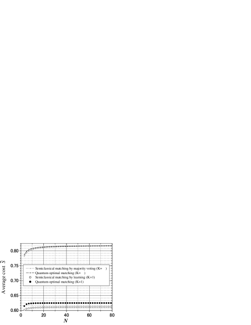
Figure 3: The average score as a function of the number of input feature systems. The big dots and circles represent the attainable scores by the universal quantum matching machine and the optimal semiclassical matching strategy based on the learning process, respectively, in the case $K=1$. The solid and dashed lines are the scores in the case of $K=\infty$ derived in our previous paper.

IV Concluding remarks

We have considered a full quantum extension of the binary quantum pattern matching problem which was addressed in the recent paper Sasaki_Carlini_Jozsa2001a . In such a problem, given unknown template states $\left|g_{1}\right\rangle^{\otimes K}$ and $\left|g_{2}\right\rangle^{\otimes K}$, and an input feature state $\left|f\right\rangle^{\otimes N}$, we are to decide to which template the input feature state is closest in the sense of the fidelity criterion. We have presented two kinds of matching strategies, that is, a semiclassical matching strategy based on learning and a universal quantum matching strategy. In particular, we have explicitly derived the Bayes optimal learning strategy for the semiclassical matching and the optimal universal quantum matching strategy in the case of one copy, $K=1$, for the template states, and an arbitrary number $N$ of copies of the input state. Our previous results in Sasaki_Carlini_Jozsa2001a correspond to the case of $K=\infty$.

For general $K\geq 2$, the Bayes optimal solutions for both the semiclassical learning strategy and the universal quantum matching strategy are still not known. Concerning the optimal learning strategy used in the semiclassical matching problem, one of the interesting questions would be whether there exists an optimal separable strategy of the type as described in Eq. (51). From a preliminary analysis of the case of $K=2$, the POM similar to Eq. (51), which is now the product made of two 3-output von Neumann measurements, does not satisfy the Bayes optimal condition for state estimation. What would then the optimal learning strategy look like in this case? Of course there should be a group covariant POM which is generally an entangled measurement on the two templates. Is such an entangled measurement the only optimal learning strategy? If so, it would be surprising because the two templates have no a priori correlation. Or are there other kinds of separable measurements? As for the universal quantum matching machine, the problem would just reduce to finding the appropriate division of the Hilbert space, but for larger $K$ this becomes a tedious task.

The reader might feel that the model used in this paper is in some respect artificial. In fact, this model is still far away from practically encountered situations. However, we may say that an important aspect of quantum pattern matching problem is already seen. Namely, there certainly exists a full quantum matching procedure as the universal quantum matching machine which is strictly superior to the straightforward extension of the conventional matching strategy based on the learning process of the classifier with the training template samples. The derived universal quantum matching machine, i.e., the POM in Eq. (124), provides a typical matching model for extracting the meaningful information about the best template class without attempting to obtain any further information about the identities of the template states themselves, excluding any intermediate measurement process. In the similar spirit, it is worth mentioning the recent work on the comparison of two unknown quantum pure states BarnettCheflesJex2002 , where the quantum optimal comparing strategies are derived for several criteria.

In practical applications, the input and the template systems will be more complicated, and possibly associated with secondary features which are not relevant to the pattern classification. So, as already pointed out in Sasaki_Carlini_Jozsa2001a , it would be of practical concern how to enhance the features of interest and to quarry the essential components (subspaces) of the quantum system for the pattern classification. In the scenario where the input and template identities are completely unknown, we might rely on a two stage procedure: first estimate the input and template identities to extract important features by using some set of aymptotically vanishing measure of the given samples; then discard redundant parts of the input and the template systems, and cut an effective subspace out of the original quantum Hilbert space; finally, after the feature enhancement process, carry out a fully quantum pattern classification procedure in the smaller space. Thus, in a sense, we see that the quantum pattern matching problem naturally involves aspects of both state estimation and state discrimination. The former is necessary for the learning process and the feature enhancement, while the latter is used for the pattern classification. In this direction, it would be also interesting to study effective quantum matching algorithms which are simple enough in structure and easy to be implemented, although not necessarily Bayes optimal.

Similarly to the case of the conventional pattern matching problem, the quantum matching algorithm complexity will be an important future problem. It is in fact believed that the complexity in some image recognition problems is in the NP-complete class. How can the quantum pattern matching problem be treated from the point of view of quantum computational complexity? If there will be some progress in the synthesis of a quantum network for the obtained optimal POM in the Bayesian approach, then it will be possible to search near optimal quantum matching algorithms whose complexity might be eventually lower than that of the corresponding conventional semiclassical approaches.

- (1) C. W. Helstrom, Quantum Detection and Estimation Theory (Academic Press, New York, 1976).
- (2) A. S. Holevo, Probabilistic and Statistical Aspects of Quantum Theory (North-Holland, Amsterdam, 1982).
- (3) A. Peres, Quantum Theory: concepts and methods (Kluwer Academic Publishers, Dortrecht, 1993).
- (4) Digital Pattern Recognition (ed. by K. S. Fu, Springer-Verlag, New York, 1976).
- (5) K. Fukunaga, Statistical Pattern Recognition (Academic Press, New York, 1990).
- (6) A. S. Holevo, J. Multivar. Anal. 3, 337 (1973).
- (7) H. P. Yuen, R. S. Kennedy, and M. Lax, IEEE Trans. IT-21, 125 (1975).
- (8) M. Sasaki, A. Carlini, and R. Jozsa, Phys. Rev. A64, 022317 (2001).
- (9) S. M. Barnett, A. Chefles, I. Jex, e-print archive, quant-ph/0202087.