Decoherence in the Heisenberg model

Abstract

We study a simplified Heisenberg spin model in order to clarify the idea of decoherence in closed quantum systems. For this purpose, we define a new concept: the decoherence function $\Xi(t)$, which describes the dynamics of decoherence in the whole system, and which is linked with the total (von Neumann) entropy of all particles. As expected, decoherence is understood both as a statistical process that is caused by the dynamics of the system, and also as a matter of entropy. Moreover, the concept of decoherence time is applicable in closed systems and we have solved its behaviour in the Heisenberg model with respect to particle number $N$, density $\rho$ and spatial dimension $D$ in a $1/r$ -type of potential. We have also studied the Poincaré recurrences occurring in these types of systems: in an $N=1000$ particle system the recurrence time is close to the order of the age of the universe. This encourages us to conclude that decoherence is the solution for quantum-classical problems not only in practice, but also in principle.

1 Introduction

Decoherence is widely accepted as an explanation of how quantum correlations are damped out to make physical systems effectively classical. Open (infinite) quantum systems have been studied in great detail by many researchers [1, 2, 3, 4, 5]. Their works are not relevant in our case, because they consider an infinite environment that consumes the quantum coherence irrevocably. But how about a finite environment or a finite system without an environment? In principle, if time is unlimited a finite system returns arbitrarily close to its starting position an infinite amount of times (Poincaré recurrence). Therefore, if a finite system starts from a superposition state it begins to lose its coherence, but will at some moment return back to its initial superposition state. Within these systems, is it reasonable to talk about decoherence, and whether there is some kind of preferred, i.e., pointer basis as Zurek calls it [6], that is realised by decoherence. If the answer is “yes”, is it somehow possible to circumvent decoherence in closed quantum systems?

Our interest in closed and finite quantum systems arises from the “cosmological” aspects of reality. The universe has no environment [3] and it has a finite number of degrees of freedom [7]. Yet decoherence is observed in our universe [8]. To understand decoherence, one should be able to model these critical aspects of the universe in decoherence studies. Previously closed quantum systems have been studied [9, 10, 11] using the frame of the many histories interpretation of quantum mechanics. This approach is, however, found to be problematic [12, 13, 14]. In this study we consider the off-diagonal elements of a reduced density matrix to avoid the problems of many histories. Another reason is that decoherence theory using reduced density matrices has not been studied in great detail, unlike the decoherent histories approach. A well established decoherence theory using reduced density matrices may clarify the concept of decoherence in closed systems. Moreover, these approaches are not equivalent [10].

Elsewhere we have analysed in detail the conceptual problem of decoherence in closed and finite systems [15]. A few major results should also be outlined here, since, they are the key concepts and premises.

1. There are two different decoherence types (similar to the different entropy types): the idealistic and the realistic decoherence.

   • The idealistic decoherence scheme can be applied only by those observers who do not interact with the universe, and who know the wave function of the universe and its time evolution. In a closed system, there is no idealistic decoherence, since the wave function of the universe remains always pure.

   • The realistic decoherence scheme is the internal view of the universe calculated from the wave function of the universe. It describes the events as the real observers that are totally correlated with the universe perceive them. To acquire this realistic viewpoint, one should make an effective theory from the wave function of the universe, e.g., to use reduced density matrices. This is often referred to as coarse-graining.

   In this study, the word “decoherence” refers to the concept of realistic decoherence. Exceptions are mentioned.

2. The possibility of recoherence does not mean that there is no decoherence. Decoherence is the decay of the off-diagonal elements of the reduced density matrix, and hence, recoherence means the growth of the off-diagonal elements of reduced density matrix. All finite quantum systems may experience recoherence.

Idealistic decoherence is often referred to with the word “decoherence”, since, in open and infinite system studies both decoherences behave similarly. The principal difference between idealistic and realistic decoherence can be seen only in closed systems.

Using a reduced-density-matrix approach, we have studied a Heisenberg spin model in order to clarify the idea of decoherence in closed systems. We focus on one particle coherence (and entropy), and thereby calculate the time evolution of the system. This coarse-graining makes our (closed) system effectively open. Within this model, it is easy to sketch how decoherence is advancing in the system. The main task of this research is to derive functional dependences of decoherence time on relevant parameters of the system (particle number $N$, density $\rho$, potential and dimension $D$ of the system), i.e., to determine how the decoherence time depends on these system variables, and why.

This paper consists of four main sections. First, we introduce our model in section 2. In section 3 we present theoretically the dynamics of a simple initial state, and define a decoherence function $\Xi(t)$ as the measure of the coherence of the whole system. Section 4 explains the structure of our simulations, along with the main results. Section 5 is for discussion.

2 The model

We have chosen the Heisenberg spin model because it is simple enough to solve, and yet complicated enough to simulate properties of real quantum systems. Coupled spin systems are interesting from a quantum computational point of view, too. Our system, $N$ interacting particles fixed in space, has no environment and, in that sense, the system forms a closed quantum universe. The particles are spin-$1\over{2}$ particles, and the interaction between them is due to their spin $z$-component (analogous to the Ising model). When there is no coupling with the environment (i.e., no outer environment), the two spin states have the same energy, which is taken to be zero. Zurek [6] and Omnès [16] have considered a similar, but simpler model in order to show that off-diagonal elements (i.e., quantum correlations) will decay in time. They labeled one particle as the system, and the others as an environment ; but, we study the particle system as a whole.

The interaction Hamiltonian,

$$H=\hbar\sum^{N-1}_{j=1}\sum^{N}_{i=j+1}g_{ij}\sigma^{j}_{z}\otimes\sigma^{i}_{z}\prod^{N}_{k=1,\neq j,i}\otimes\mathbf{1}_{k},$$ (1)

describes the dynamics of the system. The interaction matrix $G$, where $g_{ij}=g_{ji}$, gives the interaction strength between particles $i$ and $j$. The interaction strength arises from the potential $V$; but, for formal calculations there is no need to know more about it, because particles are doomed to stay in one place. Fixing the positions of the particles is a justified assumption in decoherence studies since, in most cases, the decoherence time scale is the shortest time scale [2], at least shorter than the time scale of particle motion.

3 Theoretical calculations

Let us now consider only the simplest case in order to present our method, namely initially a product state of superposition states

$$|\Psi(0)\rangle=\prod^{N}_{k=1}\otimes\left(a_{k}|+_{k}\rangle+b_{k}|-_{k}\rangle\right),$$ (2)

where $a$’s and $b$’s are normalised probability amplitudes $|a_{k}|^{2}+|b_{k}|^{2}=1$ for all $k=1,\dots,N$. The Schrödinger equation,

$$\rmi\hbar\partial_{t}|\Psi(t)\rangle=H|\Psi(t)\rangle,$$ (3)

gives the dynamics of the system, and with the given initial condition of equation (2) one gets the time dependence

$$|\Psi(t)\rangle={\rm exp}\left[-\rmi\sum^{N-1}_{j=1}\sum^{N}_{i=j+1}g_{ij}\sigma^{j}_{z}\sigma^{i}_{z}t\right]\prod^{N}_{k=1}\otimes\left(a_{k}|+_{k}\rangle+b_{k}|-_{k}\rangle\right).$$ (4)

The fate of the $l^{{\rm th}}$ particle is solved by tracing over other particles, i.e., degrees of freedom,

$$\rho_{l}={\rm Tr}_{1,\dots,N\neq l}\rho,$$ (5)

where $\rho=|\Psi(t)\rangle\langle\Psi(t)|$. This is a crucial step. We make an effective theory of our particle system by tracing over the “uninteresting” particles (that form an effective environment to the particular particle of our interest), as in the mean field approximation. The net effect of traced-out particles is described in a simpler form and with lesser degrees of freedom. This results in the particular particle under consideration being an effectively open system. The validity of this type of coarse-graining can be checked by comparing the results with the entropy studies (see section 4.3).

We thus have

$$\rho_{l} =|a_{l}|^{2}|+_{l}\rangle\langle+_{l}|+|b_{l}|^{2}|-_{l}\rangle\langle-_{l}|$$ (6)

$$+\left[a_{l}b^{*}_{l}\prod^{N}_{k=1,\neq l}\left(|a_{k}|^{2}\rme^{-\rmi 2g_{lk}t}+|b_{k}|^{2}\rme^{\rmi 2g_{lk}t}\right)|+_{l}\rangle\langle-_{l}|+h.~{}c.\right].$$

It is interesting that the result of equation (6) is the same as in reference [6], if one drops the index $l$ away. In reference [6] only an interactionless environment has been considered, but our model counts all the interactions between particles. The result of equation (6) is obvious: one particle of the system will be a victim of decoherence. In fact, all particles separately will be victims of decoherence. Other particles act as an environment for the particle of interest, and the coherence of this particular particle is dumped (i.e., displaced) temporarily into its “environment”. Now the interesting question concerns the decoherence of the whole particle system, as opposed to the decoherence of the particles separately.

The answer can be reasoned out in the following way: let us first make our notation a bit lighter by denoting

$$z_{l}=a_{l}b^{*}_{l}\prod^{N}_{k=1,\neq l}\left(|a_{k}|^{2}\rme^{-\rmi 2g_{lk}t}+|b_{k}|^{2}\rme^{\rmi 2g_{lk}t}\right).$$ (7)

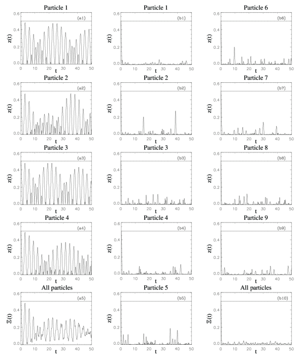
Figure 1: We illustrate two cases with different $N$: (a), $N=4$ and (b), $N=9$. For all particles $l=1,\dots,N$, $z_{l}(t)$ is plotted. We have also plotted $\Xi(t)={1\over{N}}{\sum^{N}_{l=1}|z_{l}(t)|}$ (a5, b10) which describes the decoherence of the whole system. Straight lines represent the initial states. For $N=4$, recurrences are stronger and occur more often than for $N=9$ (compare (a5) and (b10)).

This $z_{l}$ (or its complex conjugate $z^{*}_{l}$) describes the fate of the off-diagonal elements of $l^{th}$ particle. Let us put the whole system into the superposition state $a_{k}=b_{k}={1\over{\sqrt{2}}}$, $\forall k$, and let the elements of the matrix $G$ be random numbers at the interval $[0,1]$ . The time dependencies of the off-diagonal elements for all particles of the system are presented in figure 1. Note that parts of the system may come close to their starting level, but each recurs at different times. It is obvious that the whole system returns to its starting point more seldom than its parts, so the fate of all off-diagonal elements of the system is described by the function

$$\Xi(t)={1\over{N}}{\sum^{N}_{l=1}|z_{l}(t)|}.$$ (8)

We have returned to a description of the whole system; but, $\Xi(t)$ is a quantity of an effective theory, and therefore our initially closed system becomes effectively open. We are definitely describing the system from the inside view of the system, i.e., using the realistic decoherence scheme.

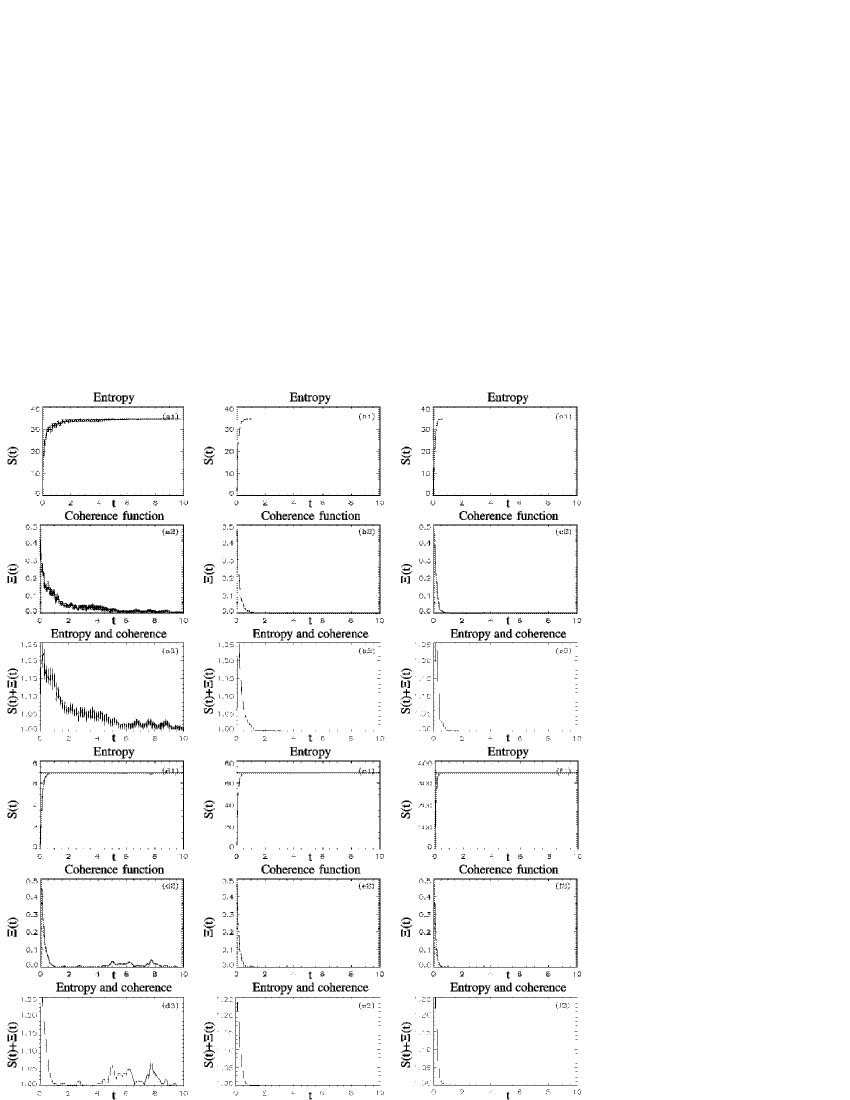
Figure 2: These figures illustrate the relation between entropy $S(t)$ (1) and coherence function $\Xi(t)$ (2). Various cases are considered (with $\rho=1$): (a) $N=50,D=1$; (b) $N=50,D=2$; (c) $N=50,D=3$; (d) $N=10,D=3$; (e) $N=100,D=3$; (f) $N=500,D=3$. It seems clear that entropy (1) and coherence function (2) are mirror images. Also the sum ${1\over{2N\ln{2}}}S(t)+\Xi(t)$ is plotted (3).

If $\Xi(t)$ achieves its initial level, the system has returned to its initial position, i.e., superpositions have recurred. The complement event of $\Xi(t)$, i.e. $Y={1\over{N}}\sum^{N}_{k=1}|a_{k}b^{*}_{k}|-\Xi(t)$, behaves as the statistical entropy in classical physics: it grows fast to some equilibrium value with certain fluctuations that depend on the number of particles in the system [in figure 2 we have presented the behaviour of $\Xi(t)$]. In open and infinite systems entropy and decoherence are related to each other (see, e.g., reference [2]), and therefore it is reasonable to assume that the same holds also in closed (and finite) systems. The decoherence function, $\Xi(t)$, is a quantity similar to the sum of all one particle (von Neumann) entropies of the system. The most stable (and the most probable) state is the one with the maximum entropy, i.e., with minimum quantum coherence. The system tends to reach this state and to spend most of its time in it. It should be clear that decoherence is a similar dynamical process as the growth of the entropy (see section 4.3); therefore, recurrences in $\Xi(t)$ are rare and short-termed phenomena.

Our model shows that decoherence is advancing at different speeds at different parts of the system. The decoherence speed of the whole particle system differs from decoherence speed of the parts of the system, and it can be evaluated from the normalised sum of all particles, i.e., $\Xi(t)$. Also, the pointer basis is realised. In our model with a particular interaction of equation (1), the pointer basis is the $\sigma_{z}$-basis. It is quite reasonable to talk about decoherence (and entropy) in a closed system.

4 Decoherence time

In infinite quantum systems, decoherence time is easily defined: it is the time when off-diagonal elements have decayed by the factor $\rme^{-1}$ (e.g. [2, 3]). If this definition is straightforwardly applied in closed systems, the following problem will appear. Decoherence is advancing at different speeds at different parts of the system, so what is the decoherence time in this case? In open systems the decay of off-diagonal elements nicely follows the function $\rme^{-t/\tau_{d}}$, where $\tau_{d}$ is decoherence time; but, in closed systems the decay function fluctuates, in some cases fluctuating a lot compared to the usual exponential behaviour. What is the decoherence time when these fluctuations are present?

We have solved this problem in the following way. First, we focus on the decoherence time of the whole system. Therefore, we use $\Xi(t)$ to solve for the decoherence time. Of course, it is also possible to pay attention only to some subsystem $S$, and solve the behaviour of this subsystem using

$$\Xi_{S}={1\over{m}}\sum^{m}_{l\in S}|z_{l}(t)|.$$ (9)

Second, we use a least squares fit on $\Xi(t)$ using a function $\xi(t)=(0.5-c)\rme^{-t/\tau_{d}}+c$ that allows fluctuations around the average level $c$. This fluctuation model is valid only when $t$ is small. “Real” time averages and fluctuations are calculated after $\Xi(t)$ has stabilised. The above mentioned decay time $\tau_{d}$ is the decoherence time. By the way, the given definition yields the same results in open and infinite systems as the familiar form ${1\over{2}}\rme^{-t/\tau_{d}}$, because in open and infinite systems $c\rightarrow 0$.

4.1 Numerics and simulations

Our main task is to try to derive the function $\tau_{d}=\tau_{d}(N,\rho,V,D)$. The starting point in our simulations is a $D$-dimensional “box” whose volume is $l^{D}$. $N$ particles are placed randomly in this box. These particles are in fixed places, and they interact with each other according to the Hamiltonian (1). In this paper, we concentrate on potentials of type

$$g_{ij}={\eta\over{|\bar{r}_{i}-\bar{r}_{j}|^{\epsilon}}},$$ (10)

where $\epsilon=1$. Now we calculate $\Xi(t)$ and fit it to the function

$$\xi(t)=(0.5-c)\rme^{-t/\tau}+c.$$ (11)

We also solve the average level of $\Xi(t)$ by calculating its time average over the interval $[t_{1},t_{2}]$, where $\tau_{d}\ll t_{1}$ and $\tau_{d}\ll t_{2}-t_{1}$:

$$\langle\Xi\rangle={1\over{t_{2}-t_{1}}}\int^{t_{2}}_{t_{1}}\Xi(t)dt.$$ (12)

This procedure is repeated $U$ times, after which we have a statistical hunch about what is going on in the box. Finally, we average acquired values of $\tau_{u}$ and $\langle\Xi\rangle_{u}$ to get a statistical estimate. $\tau_{d}={1\over{U}}\sum_{u=1}^{U}\tau_{u}$ is a function of parameters $N$, $\rho$, $V$ and $D$. Standard deviations $\sigma_{\tau_{d}}$ and $\sigma_{\langle\Xi\rangle}$ are also interesting. $\sigma_{\tau_{d}}$ is used in calculating error estimates of our model, and $\sigma_{\langle\Xi\rangle}$ describes fluctuations of $\Xi(t)$ around its average level $\langle\Xi\rangle$.

If the density under consideration is constant, then, when the number of particles is changed, the size of the box is changed, too:

$$l=\left({N\over{\rho}}\right)^{1/D}.$$ (13)

This simulation is repeated with different values of parameters $(N_{i},\rho_{i},V_{i},D_{i})$, and we get results $({\tau_{d}}_{i},\sigma_{{\tau_{d}}_{i}},\langle\Xi\rangle_{i},\sigma_{\langle\Xi\rangle_{i}})$. The next task is to find the possible underlying functional dependence.

4.2 Dependence on relevant parameters

We have focused on an initial state that contains complete superpositions, so $a_{i}=b_{i}={1\over{\sqrt{2}}}$ . The number of simulations with particular parameter values is $L=100$. Entangled particles have not (yet) been studied in relation to the case of determination of decoherence time, so our initial state is the state of equation (2). The time average is calculated in the interval of $t_{1}=50$ to $t_{2}=100$.

In this paper, we only consider the potential (10) with $\epsilon=1$. The average level of $\Xi(t)$ is only a function of $N$, and it behaves as

$$\langle\Xi\rangle(N)=A\rme^{-BN},$$ (14)

where $A\sim 1.27$ and $B\sim 0.43$. The fluctuation level around $\langle\Xi\rangle$ is the same type of function: $\sigma_{\langle\Xi\rangle}(N)=F\rme^{-GN}$, where $F\sim 0.03$ and $G\sim 0.3$.

Zurek [6] and Omnès [16] have reported that theoretical fluctuations of one particle coherence, $z(t)$, are $\sim\rme^{-N\ln{2}/2}\simeq\rme^{-0.3466N}$, so it is reasonable that our numerical results for $\Xi(t)$ behave in a similar manner.

The behaviour of decoherence time is more complicated, but it can also be analysed. The function which fits well to simulated data is

$$\tau_{d}={1\over{\eta}}\left({P\over{N^{Q}}}+R\right)\rho^{-S},$$ (15)

where $P,Q,R,S$ are fitting constants which depend on dimension $D$, and where the potential scaling factor $\eta$ is taken into account. In Table 1 we present the values of these fitting constants in dimensions $D=1,2,3$. Dimensional dependencies may be extracted from these results.

Some general results for different kinds of systems can be calculated. For $D=3$ system of $N=100$ atoms in $V=0.01~{}{\rm m^{3}}$, whose interaction strength is an electromagnetic-type interaction ($\eta\simeq 2.2\cdot 10^{6}$), the decoherence time is $\tau_{d}\sim 2\cdot 10^{-10}~{}{\rm s}$. We encourage experimentalists to do experiments with as good as possible isolated closed interacting quantum systems.

In figure 2(a2, b2, c2) differences between the dimensions are considered. The analysis shows clearly that $\Xi(t)$ describes the decoherence of the system quite well; especially when $D>1$, it follows nicely the exponential form that is typical for open and infinite quantum systems.

4.3 Recurrence

The interesting thing to notice is that our quantum system (of $N$ particles) is a closed and finite quantum system. That means, roughly speaking, that quantum correlations are never lost. They are only displaced, and the system may return to its initial state, if one waits long enough. But how much time is long enough? The answer can be reasoned out in the following way. Let us give an approximation about Poincaré recurrence time $T_{P}$ of our almost periodic function $\Xi(t)$. In reference [17] it has been argued that the period of a function of type

$$F=\sum_{i}\cos{\omega_{i}t}$$ (16)

is

$$T_{P_{F}}={2\pi\over{{\rm min}|\omega_{j}-\omega_{i}|}}.$$ (17)

This is quite elementary. The same line of thinking is applicable to the products of cosine functions, too. So, we can give an estimate of period $T_{P_{\Xi}}$ for the function of type

$$\Xi(t)={1\over{N}}\sum_{i=1}^{N}\prod_{j=1,\neq i}^{N}\cos{2g_{ij}t},$$ (18)

that is,

$$T_{P_{\Xi}}={2\pi\over{{\rm min}|\omega_{i}-\omega_{i^{\prime}}|}},$$ (19)

where $\omega_{i}=2{\rm min}|g_{ij}-g_{ij^{\prime}}|$.

The recurrence time in our simulations can be solved, and in Table 2 some examples with various $N$ and $D$ are given. The effect of $\rho$ shows up only as a common factor of $g_{ij}$ in $\omega_{i}$.

Let us study the possibility for recurrences from an entropy-based point of view. The von Neumann entropy of a particular system that is described by the density matrix $\rho$ is

$$S(\rho)=-{\rm Tr}(\rho\ln\rho).$$ (20)

The entropy of a pure state is, of course, equal to zero. Information that lies in correlations between particles is given by

$$I=\sum_{l=1}^{N}S(\rho_{l})-S(\rho),$$ (21)

where index $l$ counts subsystems, e.g., particles (see reference [18]). In our system, $S(\rho(t))\equiv 0$ because the system is closed and it starts from a pure state $|\psi(t)\rangle\langle\psi(t)|$. But the entropy of subsystems grows because the information, which is in the correlations between particles, grows. Let us now put this into a quantitative form: the total entropy of subsystems is

$$S_{tot}=\sum_{l=1}^{N}S(\rho_{l})=-\sum_{i,l}\lambda_{i,l}\ln{\lambda_{i,l}},$$ (22)

where $\lambda_{i,l}={1\over{2}}\pm{1\over{2}}\sqrt{1-4(|a_{l}|^{2}|b_{l}|^{2}-|z_{l}(t)|^{2})}$ are the eigenvalues of the reduced density matrix $\rho_{l}$. If $|a_{l}|^{2}=|b_{l}|^{2}={1\over{2}}$, then $\lambda_{i,l}={1\over{2}}\pm|z_{l}(t)|.$ In figure 2 we have plotted $S_{tot}$ with various particle numbers $N$. It is notable that the total entropy behaves as a mirror image of $\Xi(t)$. Moreover, the shape of the sum $\Xi(t)+{1\over{2N\ln{2}}}S_{tot}(t)$ is similar in every case, even if in $D=1$ there are large fluctuations present. The peak in figures 2(a3-f3) indicates that, in the beginning, the entropy grows slightly faster than decoherence, but, after the system is relaxed, they are equal. Decoherence and entropy behave regularly; they are linked to each other because they have the same origin (quantum dynamics). Our analysis shows that $\Xi(t)$ is the right concept to describe decoherence in closed and finite systems.

It seems clear that the system may return to its initial position, but the recurrence time grows fast with respect to $N$. From the entropy point of view, it is possible, in principle, for the system to get completely to the initial state again, but, it is thermodynamically impossible, i.e., the recurrence time is much greater than the age of the universe.

5 Discussion

We have studied this simple scenario in order to clarify the idea of decoherence in closed systems. We have stated that decoherence and entropy are two sides of the same coin: they are well defined inside (effective theory) descriptions of the closed system. This effective theory of a closed system is valid for observers inside the universe, i.e., they observe a truly closed and finite universe as effectively open. The universe is truly closed from an outside point of view (complete description), but the only way to access this view is an academic example. We leave the detailed analysis of different types of observers in complete and effective theories for elsewhere. Still, decoherence is a working concept in closed systems also in principle, not only in practice, e.g., as Bell has argued [16, 19]. Bell’s argument against decoherence has been refuted (e.g., by Omnès [16]) .

The possibility of recurrence makes neither concept, entropy nor decoherence, empty. Decoherence is a dynamical process, arising from interactions between particles, that diagonalises reduced density matrices in the pointer basis. This holds true in our model. Decoherence time $\tau_{d}$ can be applied and determined in closed systems as well as in open systems, and the function $\Xi(t)$ describes the fate of all off-diagonal elements of particles forming the system. $\Xi(t)$ can be linked with the entropy of the system as a mirror image. The particles-in-a-box example in classical statistical physics is analogous to decoherence: the recurrence of all off-diagonal elements in our system is a similar kind of phenomenon to the gas in a closed chamber going completely to the other half of the chamber. This is possible, but its possibility diminishes as $N$ grows. In the complete description (view from outside), the total entropy and the idealistic quantum coherence of a closed system are constants, but in the effective theory (view from inside) sums of both realistic quantities are evolving in time, as described in Sections 4.2 and 4.3.

It is quite obvious that the decoherence time $\tau_{d}$ behaves as $\sim N^{-Q}$ and $\sim\rho^{-S}$, because decoherence is faster in bigger systems (many particles and high density) than in small systems. An interesting feature is that the decoherence time with respect to $N$ saturates to a certain value $R$ that is dimension-dependent. Using equation (15) one can argue that an $N\sim 43000$ $3D$-particle system behaves as an infinite particle system with an accuracy of $99\%$. The amount of particles needed to cause a nearly-infinite type of behaviour is small compared to the baryon number of our universe ($\sim 10^{80}$ [7]). The saturation effect gives in principle a possibility to fight against decoherence: just make a low density system. Of course, vacuum fluctuations are present in low density cases, and therefore studies of the effects of second quantisation are important in fighting decoherence.

With our model, it is possible study the Schrödinger cat experiment which crucially showed the problems in understanding quantum mechanics and the demarcation problem between quantum and classical [20]. Many improvements have been made in quantum mechanics since the days of Schrödinger, especially concerning decoherence. This study covers basically the question of quantum-classical problem; we have shown that quantum mechanics can be applied to the whole universe, and as an effective theory we acquire almost a classical universe with the help of decoherence. The Schrödinger cat problem is more than this demarcation problem, but the presented model can be used in constructing a realistic enough model of a cat and its surroundings. Entangled states will play a crucial role in that case.

The “cat-in-the-box” will be in our future interests, as well as other $1/r^{\epsilon}$ potentials. Also, ideas how to circumvent decoherence are interesting. The system geometry may play some role in slowing down decoherence and making recurrence more probable. Correlations between particles should be studied as well in greater detail; here we have only considered an effective theory with one-particle correlations, but many-particle correlations may contribute to the dynamics of the system. However, our entropy studies seem to justify the results. There is one minor drawback in our model that is a result of simplifying and making an academic example, and it may affect the results: the model is, strictly speaking, discrete because the particles are placed (randomly, but this does not matter) in fixed and accurate places. Clearly, this violates the Heisenberg uncertainty principle and may cause considerable effects. It would be interesting to study what kind of results are acquired with particles as probability distributions in space.

References

Tables and table captions

Table 1: The values of fitting constants. Some constants follow (within the error bars which are acquired from our statistical analysis) a dimensional scaling which is presented on the last row.

• $D$	$P$	$Q$	$R$	$S$
  1	$3.73\pm 1.0$	$1.49\pm 0.3$	$0.415\pm 0.022$	$1.80\pm 0.05$
  2	$0.77\pm 0.3$	$0.80\pm 0.1$	$0.166\pm 0.004$	$1.00\pm 0.05$
  3	$0.45\pm 0.1$	$0.55\pm 0.05$	$0.128\pm 0.003$	$0.67\pm 0.05$
  Scaling	$3.5/D^{2}$	$1.6/D$		$1.80/D^{0.88}$

Table 2: Examples of estimated recurrence times $T_{P_{\Xi}}$ with various initial conditions. We have also presented standard deviations of these numerically estimated recurrence times. Note that $T_{P_{\Xi}}$ is highly dependent on $N$ and $D$. The unit of time is $gt$.

• $N$	$\rho$	$D$	$T_{P_{\Xi}}$	$\sigma_{T_{P_{\Xi}}}$
  10	1	1	$5.0\cdot 10^{6}$	$1.1\cdot 10^{8}$
  50	1	1	$4.6\cdot 10^{10}$	$2.7\cdot 10^{11}$
  100	1	1	$2.2\cdot 10^{12}$	$1.2\cdot 10^{13}$
  500	1	1	$6.3\cdot 10^{16}$	$3.6\cdot 10^{17}$
  1000	1	1	$5.5\cdot 10^{17}$	$1.9\cdot 10^{18}$
  1000	1	2	$2.2\cdot 10^{15}$	$4.7\cdot 10^{15}$
  1000	1	3	$4.0\cdot 10^{14}$	$8.6\cdot 10^{14}$
  1000	10	3	$2.0\cdot 10^{14}$	$4.5\cdot 10^{14}$

Figures and figure captions

References

- [1] Caldeira A O and Leggett A J 1983 Physica A 121 587; 1985 Phys. Rev. A 31 1059
- [2] Unruh W G and Zurek W H 1989 Phys. Rev. D 40 1071
- [3] Zurek W H 1991 Phys. Today 44(10) 36
- [4] Hu B L, Paz J P and Zhang Y 1992 Phys. Rev. D 45 2843
- [5] Anglin J R, Laflamme R, Zurek W H and Paz J P 1995 Phys. Rev. D 52 2221
- [6] Zurek W H 1982 Phys. Rev. D 26 1862
- [7] Lloyd S 2002 Phys. Rev. Lett. 88 237901
- [8] Brune M, Hagley E, Dreyer J, Maître X, Maali A, Wunderlich C, Raimond J M and Haroche S 1996 Phys. Rev. Lett. 77 4887
- [9] Dowker H F and Halliwell J J 1992 Phys. Rev. D 46 1580
- [10] Gell-Mann M and Hartle J B 1993 Phys. Rev. D 47 3345
- [11] Brun T A and Hartle J B 1999 Phys. Rev. D 60 123503
- [12] Dowker H F and Kent A 1996 J. Stat. Phys. 82 1575
- [13] Kent A 1996 Phys. Rev. A 54 4670
- [14] Kent A 1997 Phys. Rev. Lett. 78 2874
- [15] Dannenberg O 2003 Unpublished
- [16] Omnès R 1994 The Interpretation of Quantum Mechanics (Princeton University Press, Princeton)
- [17] Gaioli F H, Alvarez E T G and Guevara J 1997 Int. J. Theor. Phys. 36 2167
-
[18]
Preskill J 1998
Quantum Information and Computation (lecture notes for physics
229),
http://www.theory.caltech.edu/preskill/ph229 - [19] Bell J S 1975 Helv. Phys. Acta 48 93
- [20] Schrödinger E 1935 Die Naturwissenschaften 23 807-812, 823-828, 844-849