Quantum properties of transverse pattern formation in second-harmonic generation

Abstract

We investigate the spatial quantum noise properties of the one dimensional transverse pattern formation instability in intra-cavity second-harmonic generation. The Q representation of a quasi-probability distribution is implemented in terms of nonlinear stochastic Langevin equations. We study these equations through extensive numerical simulations and analytically in the linearized limit. Our study, made below and above the threshold of pattern formation, is guided by a microscopic scheme of photon interaction underlying pattern formation in second-harmonic generation. Close to the threshold for pattern formation, beams with opposite direction of the off-axis critical wave numbers are shown to be highly correlated. This is observed for the fundamental field, for the second harmonic field and also for the cross-correlation between the two fields. Nonlinear correlations involving the homogeneous transverse wave number, which are not identified in a linearized analysis, are also described. The intensity differences between opposite points of the far fields are shown to exhibit sub-Poissonian statistics, revealing the quantum nature of the correlations. We observe twin beam correlations in both the fundamental and second-harmonic fields, and also nonclassical correlations between them.

I Introduction

Pattern formation has been an active area of research in many diverse systems [1]. Numerous similarities to pattern formation in other systems have been reported in recent studies in nonlinear optics [2, 3, 4, 5, 6]. However similar, nonlinear optics also displays properties that are wholly unique due to the relevance of quantum aspects in optical systems, one manifestation of this is the inevitable quantum fluctuations of light. In the last decade an effort has been made to study the interplay in the spatial domain between optical pattern formation, known from classical nonlinear optics, and the quantum fluctuations of light [7, 8]. New nonclassical effects such as quantum entanglement and squeezing in patterns were predicted [8, 9]. Another interesting example is the phenomenon of quantum images: below the instability threshold, information about the pattern is encoded in the way the quantum fluctuations of the fields are spatially correlated [10].

Nonlinear $\chi^{(2)}$-materials immersed in a cavity have shown most promising quantum effects. A paradigm of spatiotemporal quantum behavior has been the optical parametric oscillator (OPO), which despite its striking simplicity is able to display highly complex behavior [11, 12, 13]. In the degenerate OPO, pump photons are down-converted to signal photons at half the frequency and with a high degree of quantum correlation. This might be attributed to the fact that the signal photons are created simultaneously conserving energy and momentum, leading to the notion of twin photons. In the opposite process of second-harmonic generation (SHG) fundamental photons are up-converted to second-harmonic photons at the double frequency. On a classical level, both the OPO and intra-cavity SHG display similar spatiotemporal behavior. The essential difference between them is that in the OPO an oscillation threshold for the process exists, which simultaneously acts as the threshold for pattern formation. On the contrary, SHG always takes place no matter the strength of the pump field, but there is a threshold that marks the onset of pattern formation. This gives pronounced differences with the OPO in the linearized behavior below the threshold for pattern formation. In the OPO the pump and the signal fields effectively decouple and only the latter becomes unstable at threshold. At a microscopic level, the behavior of the OPO close to the threshold can be understood in terms of a unique process in which a pump photon decays into two signal photons with opposite wave numbers. In SHG the fundamental and second-harmonic fields are coupled and both become unstable at threshold. This complicates the picture mainly by the number of microscopic mechanisms that are relevant to describe the pattern formation process. But this complexity, on the other hand, is likely to generate interesting correlations between the fundamental and the second-harmonic field. Recently, transverse quantum properties in the singly resonant SHG setup were investigated [14]. There, squeezing in the fundamental output was observed close to the critical wave number, but since the second-harmonic is not resonated the question of possible correlations between the two fields was not addressed. However, since the second harmonic in the singly resonant case is given directly as a function of the fundamental, correlations similar to the ones observed in the fundamental should be expected. In this paper, we will consider the case of doubly resonant SHG with the aim of investigating the spatial correlations not only within each field (fundamental field and second-harmonic field), but also between the two fields.

For this purpose we use the formalism of quasi-probability distributions [15]. Choosing the use of the Q representation we are able to derive a set of nonlinear Langevin equations that describes the time evolution of the quantum fields in the SHG setup (Sec. II). In Sec. III, the linear stability analysis of this system will be discussed and a proper regime of parameters specified, for which the formalism adopted here is applicable. Section IV will be devoted to an analysis, on a microscopic level, of the implications of the three-wave interactions in the nonlinear crystal. These considerations allow to identify the most important spatial correlations expected in this two-field system and to define suitable quantities to be calculated. In particular, we will focus on equal time correlation functions of intensity fluctuations and we will study photon number variances when looking for nonclassical features of the intra-cavity fields. A systematic study of the spatial correlations is presented first through analytical results in the framework of a linearized theory below the threshold for pattern formation (Sec. V), and also through extensive numerical simulations of the nonlinear Langevin equations reported below (Sec. VI) and above (Sec. VII) the threshold for pattern formation. We conclude in Sec. VIII.

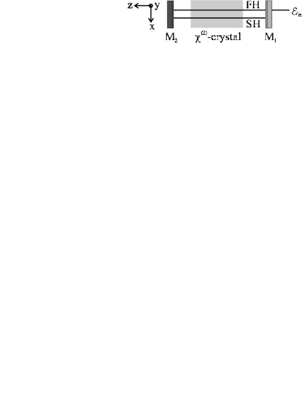
FIG. 1.: The model setup in a top-view.

II Nonlinear quantum model for intra-cavity SHG

We consider a nonlinear $\chi^{(2)}$-material with type I phase matching immersed in a cavity with a high reflection input mirror $M_{1}$ and a fully reflecting mirror $M_{2}$ at the other end, cf. Fig. 1. The cavity is pumped at the frequency $\omega_{1}$ and through the nonlinear interaction in the crystal photons of frequency $\omega_{2}=2\omega_{1}$ are generated. This is the process of SHG. The cavity supports a discrete number of longitudinal modes, and we will consider the case where only two of these modes are relevant, namely the mode $\omega_{1,{\mathrm{c}av}}$ closest to the fundamental frequency and $\omega_{2,{\mathrm{c}av}}$ closest to the second-harmonic frequency. In the setup shown in Fig. 1 $\omega_{2,{\mathrm{c}av}}=2\omega_{1,{\mathrm{c}av}}$, but we will allow the cavity resonances to be independent in order to control the detunings individually. The pump beam propagates along the $z$-direction and using the mean field approximation, variations in the $z$-direction are averaged out. This approach is justified as long as the losses and detunings are small. Due to diffraction the transverse section perpendicular to the $z$-direction spanned by the $xy$-plane also comes into play. We consider the simple 1D case where only one of the transverse directions is relevant, so variations along the $y$-direction are neglected and only the $x$-direction is taken into account (this could easily be achieved experimentally by using a crystal with a small height). Let $\hat{A}_{1}(x,t)$ and $\hat{A}_{2}(x,t)$ denote the 1D intra-cavity boson operators of the fundamental field (FH) and second-harminic field (SH), respectively. They obey the following equal time commutation relation

$$[\hat{A}_{i}(x,t),\hat{A}_{j}^{\dagger}(x^{\prime},t)]=\delta_{ij}\delta(x-x^{\prime}),\quad i,j=1,2.$$ (1)

The Hamiltonian operator describing SHG including diffraction can be written as done in Ref. [13] for the OPO,

$$\hat{H}=\hat{H}_{\mathrm{f}ree}+\hat{H}_{\mathrm{i}nt}+\hat{H}_{\mathrm{e}xt},$$ (2)

where the free Hamiltonian is given by

$$\hat{H}_{\mathrm{f}ree} = \hbar\int dx\hat{A}_{1}^{\dagger}(x,t)\left(-\delta_{1}-\frac{c^{2}}{2\omega_{1}}\frac{\partial^{2}}{\partial x^{2}}\right)\hat{A}_{1}(x,t)$$ (4)

$$+\hbar\int dx\hat{A}_{2}^{\dagger}(x,t)\left(-\delta_{2}-\frac{c^{2}}{4\omega_{1}}\frac{\partial^{2}}{\partial x^{2}}\right)\hat{A}_{2}(x,t).$$

Here $\delta_{j}=\omega_{j}-\omega_{j,{\mathrm{c}av}}$ are the detunings from the nearest cavity resonances, $\partial^{2}/\partial x^{2}$ describes the diffraction, and $c$ is the speed of light. The interaction Hamiltonian describes the nonlinear interaction in the material

$$\hat{H}_{\mathrm{i}nt}=\frac{i\hbar g}{2}\int dx\left(\hat{A}_{2}(x,t)({\hat{A}}_{1}^{\dagger}(x,t))^{2}-{\mathrm{H}.c.}\right),$$ (5)

where $g$ is the nonlinear coupling parameter proportional to the $\chi^{(2)}$-nonlinearity of the crystal. The external Hamiltonian describes the effects of the pump injected into the cavity at the fundamental frequency, which is taken to be a classical quantity ${\mathcal{E}}_{\mathrm{i}n}$, so we have

$$\hat{H}_{\mathrm{e}xt}=i\hbar\int dx\left({\mathcal{E}}_{\mathrm{i}n}\hat{A}_{1}^{\dagger}(x,t)-{\mathcal{E}}_{\mathrm{i}n}^{*}\hat{A}_{1}(x,t)\right).$$ (6)

Then the master equation for the density matrix $\hat{\rho}$ in the interaction picture is given by

$$\frac{\partial\hat{\rho}}{\partial t}=-\frac{i}{\hbar}[\hat{H},\hat{\rho}]+(\hat{L}_{1}+\hat{L}_{2})\hat{\rho}.$$ (7)

The cavity losses are assumed to occur only through the input coupling mirror to the external continuum of modes, and are here included through the Liouvillian terms

$$\hat{L}_{j}\hat{\rho}= \int dx\gamma_{j}\Big{(}2\hat{A}_{j}(x,t)\hat{\rho}\hat{A}_{j}^{\dagger}(x,t)$$ (9)

$$-\hat{\rho}\hat{A}_{j}^{\dagger}(x,t)\hat{A}_{j}-\hat{A}_{j}^{\dagger}(x,t)\hat{A}_{j}(x,t)\hat{\rho}\Big{)},$$

where $\gamma_{j}$ are the cavity loss rates. Here we have assumed that thermal fluctuations in the system can be neglected.

Using the standard approach of expanding the density matrix into coherent states weighted by a quasi-probability distribution function, the master equation (7) is mapped onto a functional equation, depending on the order for creation and destruction operators [16, 17]. For a Hamiltonian that is quadratic in the field operators this results in a Fokker-Planck equation, implying that the dynamical evolution of the distribution function may be modelled by an equivalent set of classical stochastic Langevin equations. However, due to the contributions of higher order to the Hamiltonian (5) problems may arise. When using the Wigner representation the evolution equation of the quasi-probability functional contains third order derivatives, which means that no equivalent Langevin equations can be found. These third order terms have been shown to model quantum jump processes [18]. In some cases these terms can be neglected leading to an approximate Fokker-Planck form. When using the P or Q representations problems of negative diffusion in the Fokker-Planck equation come into play [15]. To avoid negative diffusion in the P representation, some techniques have been developed where the phase space is doubled [19, 20], but then numerical problems due to divergent stochastic trajectories generally appear [21, 22]. We choose here to use the Q representation which in a restricted domain of parameters has a nonnegative diffusion matrix and has been shown to be a useful alternative in the similar problem of calculating nonlinear quantum correlations in the OPO [23]. The Q representation has no singularity problems, is bounded and always nonnegative.

Introducing $\alpha_{i}$ and $\alpha_{i}^{*}$ as the c-number equivalents of the intra-cavity boson operators $\hat{A}_{i}$ and $\hat{A}_{i}^{\dagger}$, the evolution equation for the quasi-probability distribution function $Q(\underline{\alpha})$ is

$$\frac{\partial Q(\underline{\alpha})}{\partial t} =\Bigg{(}\frac{\partial}{\partial\alpha_{1}}[(\gamma_{1}-i\delta_{1})\alpha_{1}-g\alpha_{1}^{*}\alpha_{2}-i\frac{c^{2}}{2\omega_{1}}\frac{\partial^{2}}{\partial x^{2}}-{\mathcal{E}}_{{\mathrm{i}n}}]$$ (10)

$$+ \frac{\partial}{\partial\alpha_{2}}[(\gamma_{2}-i\delta_{2})\alpha_{2}+\frac{g}{2}\alpha_{1}^{2}-i\frac{c^{2}}{4\omega_{1}}\frac{\partial^{2}}{\partial x^{2}}]-\frac{g}{2}\alpha_{2}\frac{\partial^{2}}{\partial\alpha_{1}^{2}}$$ (11)

$$+ \gamma_{1}\frac{\partial^{2}}{\partial\alpha_{1}\partial\alpha_{1}^{*}}+\gamma_{2}\frac{\partial^{2}}{\partial\alpha_{2}\partial\alpha_{2}^{*}}+{\mathrm{c}.c.}\Bigg{)}Q(\underline{\alpha}),$$ (12)

with $\underline{\alpha}=\{\alpha_{1},\alpha_{1}^{*},\alpha_{2},\alpha_{2}^{*}\}$. This is just an extension to the diffractive case of the result obtained by Savage [24]. Equation (10) has the form of a Fokker-Planck equation, and it has positive diffusion if

$$|\alpha_{2}|<2\frac{\gamma_{1}}{g}.$$ (13)

As shown below, it is possible to fix the parameters of the system in such a way that the stable solution for the SH field is well below the value $2\gamma_{1}/g$. Fluctuations around this stable solution are small, so that the probability violating the condition (13) is almost zero. Neglecting then stochastic trajectories violating this condition, we may write a set of equivalent Langevin stochastic equations by applying the Ito formalism for the stochastic integration [25]. We then obtain the following nonlinear Langevin equations

$$\partial_{t}\alpha_{1}(x,t)= (-\gamma_{1}+i\delta_{1})\alpha_{1}(x,t)+g\alpha_{1}^{*}(x,t)\alpha_{2}(x,t)$$ (16)

$$+i\frac{c^{2}}{2\omega_{1}}\frac{\partial^{2}}{\partial x^{2}}\alpha_{1}(x,t)+{\mathcal{E}}_{\mathrm{i}n}+\sqrt{2\gamma_{1}}\xi_{1}(x,t),$$

$$\partial_{t}\alpha_{2}(x,t)= (-\gamma_{2}+i\delta_{2})\alpha_{2}(x,t)-\frac{g}{2}\alpha_{1}^{2}(x,t)$$ (18)

$$+i\frac{c^{2}}{4\omega_{1}}\frac{\partial^{2}}{\partial x^{2}}\alpha_{2}(x,t)+\sqrt{2\gamma_{2}}\xi_{2}(x,t),$$

with multiplicative Gaussian white noise sources correlated as follows

$$\langle\xi_{i}^{*}(x,t)\xi_{j}(x^{\prime},t^{\prime})\rangle = \delta_{ij}\delta(x-x^{\prime})\delta(t-t^{\prime}),$$ (20)

$$\langle\xi_{2}(x,t)\xi_{2}(x^{\prime},t^{\prime})\rangle = 0,$$ (21)

$$\langle\xi_{1}(x,t)\xi_{1}(x^{\prime},t^{\prime})\rangle = -\frac{g\alpha_{2}(x,t)}{2\gamma_{1}}\delta(x-x^{\prime})\delta(t-t^{\prime}).$$ (22)

We rescale space and time according to

$$\tilde{t}=t\gamma_{1},\quad\tilde{x}=x/l_{d},$$ (23)

where $l_{d}$ is the characteristic length scale given by

$$l_{d}^{2}=\frac{c^{2}}{2\gamma_{1}\omega_{1}}.$$ (24)

We also normalize the fields and noise according to

$$A_{j}(x,t)=\alpha_{j}(x,t)\frac{g}{\gamma_{1}},\quad\tilde{\xi}_{j}(x,t)=\xi_{j}(x,t)\sqrt{\frac{l_{d}}{\gamma_{1}}},$$ (25)

$$E={\mathcal{E}}_{\mathrm{i}n}\frac{g}{\gamma_{1}^{2}}.$$ (26)

This allows to rewrite the Langevin equations in dimensionless form:

$$\partial_{\tilde{t}}A_{1}(\tilde{x},\tilde{t}) = (-1+i\Delta_{1})A_{1}(\tilde{x},\tilde{t})+A_{1}^{*}(\tilde{x},\tilde{t})A_{2}(\tilde{x},\tilde{t})$$ (29)

$$+i\frac{\partial^{2}}{\partial\tilde{x}^{2}}A_{1}(\tilde{x},\tilde{t})+E+\sqrt{\frac{2}{n_{th}}}\tilde{\xi}_{1}(\tilde{x},\tilde{t}),$$

$$\partial_{\tilde{t}}A_{2}(\tilde{x},\tilde{t}) = (-\gamma+i\Delta_{2})A_{2}(\tilde{x},\tilde{t})-\frac{1}{2}A_{1}^{2}(\tilde{x},\tilde{t})$$ (31)

$$+\frac{i}{2}\frac{\partial^{2}}{\partial\tilde{x}^{2}}A_{2}(\tilde{x},\tilde{t})+\sqrt{\frac{2\gamma}{n_{th}}}\tilde{\xi}_{2}(\tilde{x},\tilde{t}),$$

where $\gamma=\gamma_{2}/\gamma_{1}$ and $\Delta_{j}=\delta_{j}/\gamma_{1}$, and $E$ may be taken real. Moreover we have introduced

$$n_{th}=\frac{\gamma_{1}^{2}l_{d}}{g^{2}},$$ (32)

which in the OPO coincides with the number of photons in the characteristic “area” $l_{d}$ required to trigger the oscillation. The noise strength is seen to scale like $n_{th}^{-1/2}$. The normalized noise sources are correlated by

$$\langle\tilde{\xi}_{i}^{*}(\tilde{x},\tilde{t})\tilde{\xi}_{j}(\tilde{x}^{\prime},\tilde{t}^{\prime})\rangle = \delta_{ij}\delta(\tilde{x}-\tilde{x}^{\prime})\delta(\tilde{t}-\tilde{t}^{\prime}),$$ (34)

$$\langle\tilde{\xi}_{2}(\tilde{x},\tilde{t})\tilde{\xi}_{2}(\tilde{x}^{\prime},\tilde{t}^{\prime})\rangle = 0,$$ (35)

$$\langle\tilde{\xi}_{1}(\tilde{x},\tilde{t})\tilde{\xi}_{1}(\tilde{x}^{\prime},\tilde{t}^{\prime})\rangle = -\frac{A_{2}(\tilde{x},\tilde{t})}{2}\delta(\tilde{x}-\tilde{x}^{\prime})\delta(\tilde{t}-\tilde{t}^{\prime}).$$ (36)

These noise sources turn out to only to be defined for

$$|A_{2}(\tilde{x},\tilde{t})|<2,$$ (37)

which coincides with the condition (13) for a positive diffusion expressed in terms of the rescaled fields.

In the following the tildes are dropped, and only normalized dimensionless equations are considered. We will also use the terminology $\omega\equiv\omega_{1}$ and $2\omega\equiv\omega_{2}$.

III Linearized equations and bifurcation diagram

In this section we consider the linearization of the nonlinear Langevin equations in the Q representation around the homogeneous steady state solutions below the threshold for pattern formation. This approach relies on the assumption that the fluctuations are small with respect to the field mean values, and therefore we expect this approach to break down close to the instability threshold. We will come back later (Sec. VI B) to the question of the validity of the linear approximation. We write the fields as $A_{j}(x,t)={\mathcal{A}}_{j}+\beta_{j}(x,t)$, where $\beta_{j}(x,t)$ represent the fluctuations around ${\mathcal{A}}_{j}$. The classical homogeneous values ${\mathcal{A}}_{j}$ of the fields given by the homogeneous steady state solutions of the deterministic limit ($n_{th}\rightarrow\infty$) of Eqs. (II), as found in Ref.[6]. Using this in Eqs. (II) we find the following set of linearized equations

$$\partial_{t}\beta_{1}(x,t) = (-1+i\Delta_{1})\beta_{1}(x,t)+{\mathcal{A}}_{2}\beta_{1}^{*}(x,t)$$ (39)

$$+ {{\mathcal{A}}^{*}_{1}}\beta_{2}(x,t)+i\frac{\partial^{2}}{\partial x^{2}}\beta_{1}(x,t)+\sqrt{\frac{2}{n_{th}}}\xi_{1}(x,t),$$ (40)

$$\partial_{t}\beta_{2}(x,t) = (-\gamma+i\Delta_{2})\beta_{2}(x,t)-{\mathcal{A}}_{1}\beta_{1}(x,t)$$ (41)

$$+ \frac{i}{2}\frac{\partial^{2}}{\partial x^{2}}\beta_{2}(x,t)+\sqrt{\frac{2\gamma}{n_{th}}}\xi_{2}(x,t).$$ (42)

The correlations of the stochastic sources $\xi_{i}(x,t)$ in the linearized limit become

$$\langle\xi_{i}^{*}(x,t)\xi_{j}(x^{\prime},t^{\prime})\rangle = \delta_{ij}\delta(x-x^{\prime})\delta(t-t^{\prime}),$$ (44)

$$\langle\xi_{1}(x,t)\xi_{1}(x^{\prime},t^{\prime})\rangle = -\frac{{\mathcal{A}}_{2}}{2}\delta(x-x^{\prime})\delta(t-t^{\prime}),$$ (45)

$$\langle\xi_{2}(x,t)\xi_{2}(x^{\prime},t^{\prime})\rangle = 0.$$ (46)

With ${\mathcal{A}}_{2}$ being merely a constant, the noise in the linear approximation is not multiplicative any more. However, as in the nonlinear equations we have the restriction

$$|{\mathcal{A}}_{2}|<2.$$ (47)

We would like to mention that the Wigner representation, in the linear regime, would lead to equivalent results without suffering from any limitation since it satisfies a Fokker-Planck equation for any value of $|{\mathcal{A}}_{2}|$. However, for the sake of a consistent presentation of our results we have chosen to consider the Q representaion also in the linear case.

It is instructive to introduce the spatial Fourier transform of the fluctuations

$$\beta_{j}(k,t)=\int_{-\infty}^{\infty}\frac{dx}{\sqrt{2\pi}}\beta_{j}(x,t)e^{ikx},$$ (48)

which physically represents the amplitude of the fluctuations in the far field. Considering Eqs. (III) and their complex conjugates, it is readily shown that these amplitudes $\beta_{j}(k,t)$ fulfill a set of equations which can be written in the following matrix form

$$\partial_{t}\left(\begin{array}[]{c}\beta_{1}(k,t)\\ \beta_{1}^{*}(-k,t)\\ \beta_{2}(k,t)\\ \beta_{2}^{*}(-k,t)\end{array}\right)={\mathbf{M}}(k)\left(\begin{array}[]{c}\beta_{1}(k,t)\\ \beta_{1}^{*}(-k,t)\\ \beta_{2}(k,t)\\ \beta_{2}^{*}(-k,t)\end{array}\right)$$ (58)

$$+\sqrt{\frac{2}{n_{th}}}\left(\begin{array}[]{c}\eta_{1}(k,t)\\ \eta_{1}^{*}(-k,t)\\ \sqrt{\gamma}\eta_{2}(k,t)\\ \sqrt{\gamma}\eta_{2}^{*}(-k,t)\end{array}\right),$$ (63)

$${\mathbf{M}}(k)=\left(\begin{array}[]{cccc}\sigma_{1}(k)&{\mathcal{A}}_{2}&{\mathcal{A}}_{1}^{*}&0\\ {\mathcal{A}}_{2}^{*}&\sigma_{1}^{*}(k)&0&{\mathcal{A}}_{1}\\ -{\mathcal{A}}_{1}&0&\sigma_{2}(k)&0\\ 0&-{\mathcal{A}}_{1}^{*}&0&\sigma_{2}^{*}(k)\\ \end{array}\right),$$ (68)

where $\sigma_{1}(k)=-1+i(\Delta_{1}-k^{2})$ and $\sigma_{2}(k)=-\gamma+i(\Delta_{2}-k^{2}/2)$ have been introduced and each noise term $\eta_{j}(k,t)$ is the Fourier transform of the noise term appearing in the real space linearized Langevin equations (III). Their correlations are given by

$$\langle\eta_{i}^{*}(k,t)\eta_{j}(k^{\prime},t^{\prime})\rangle = \delta_{ij}\delta(k-k^{\prime})\delta(t-t^{\prime}),$$ (70)

$$\langle\eta_{1}(k,t)\eta_{1}(k^{\prime},t^{\prime})\rangle = -\frac{{\mathcal{A}}_{2}}{2}\delta(k+k^{\prime})\delta(t-t^{\prime}),$$ (71)

$$\langle\eta_{2}(k,t)\eta_{2}(k^{\prime},t^{\prime})\rangle = 0.$$ (72)

The linear stability of the classical equations obtained as the $n_{th}\rightarrow\infty$ limit of Eqs. (III) was investigated by Etrich et al. [6]. A rich variety of instabilities was shown to exist: A self-pulsing instability, that leads to oscillations of the homogeneous steady states without any transverse structure, was present for all parameters. The oscillatory transverse instability leading to patterns traveling in space and time was only present for certain parameters and branched out from the self-pulsing instability. Bistability was demonstrated for large detunings of same sign and for $\gamma$ small. Most importantly, for all parameters also stationary transverse instabilities were found to exist, i.e. instabilities at a critical transverse wave number $k=k_{c}$ and with zero imaginary eigenvalue. It was shown that stripe-type solutions exist but are always unstable, and numerical simulations showed that instead hexagons are the dominating stationary transverse instability. The 1D configuration we have chosen to consider here has the advantage that the pattern always will be a stripe and therefore leads to simpler interpretation of the correlations. We will choose a range of parameters in which the stationary transverse instability is accessible as the primary bifurcation. This bifurcation is supercritical in the 1D model.

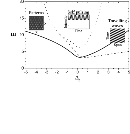
FIG. 2.: Stability diagram for $\Delta_{1}=2.0$ and $\gamma=0.5$, showing transverse stationary instability (solid line), transverse oscillatory instability (dashed line) and self-pulsing instability (dotted line).

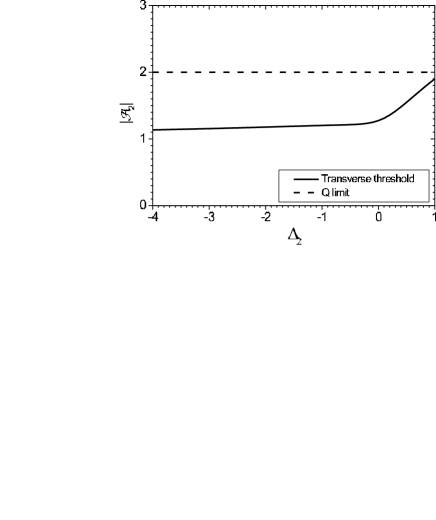
FIG. 3.: Transverse instability for $\Delta_{1}=2.0$ and $\gamma=0.5$ shown for the intra-cavity second-harmonic field, along with the limit for the Q representation, $|A_{2}|<2$.

The choice of parameters must take into account the requirement of applicability of the Q representation. One finds that Eq. (47) can only be satisfied for $\Delta_{1}>0$ [26]. Using the expressions presented in Ref. [6] and fixing $\Delta_{1}=2.0$ and $\gamma=0.5$ we obtain the bifurcation diagram shown in Fig. 2 [27]. We observe that for $\Delta_{2}<0$ it is possible to obtain stationary patterns (solid line) as the primary bifurcation at a critical value of the pump, $E_{t}$; increasing the pump beyond $E_{t}$ eventually the system will also become self-pulsing unstable (dotted line). For $\Delta_{2}>0$ the transverse oscillatory bifurcation (dashed line) is the primary one, and therefore travelling waves are observed in this region. The bistable area is located for $\Delta_{2}>8.3$ and hence beyond the range shown here.

Expressing the onset of transverse instability, seen in Fig. 2, in terms of the intra-cavity value of the SH we have the bifurcation diagram for the transverse instability shown in Fig. 3. We see that for $\Delta_{2}<0$ we are well below the limit for positive diffusion (47). Therefore, the probability of trajectories violating the condition (37) of the nonlinear equations is almost zero. For $\Delta_{2}>0$, increasing $\gamma$ or decreasing $\Delta_{1}$ towards zero, this threshold gets closer to $|{\mathcal{A}}_{2}|=2$.

We will therefore use the parameters $\Delta_{1}=2.0$, $\Delta_{2}=-2.0$ and $\gamma=0.5$ in the rest of this paper, which gives a pattern formation threshold of $E_{t}=7.481757$ and a critical wave number $k_{c}=1.833$. The noise strength is set to $n_{th}=10^{8}$ which is a typical value for the cavity setup discussed here [28].

FIG. 4.: Numerical simulation of the Langevin equations above threshold with $E/E_{t}=1.01$ and $L=102.84$. Left: The absolute value of the near field of the FH (above) and SH (below). Right: Far field average intensity of FH, $\langle|A_{1}(k)|^{2}\rangle$. The far field of the SH shows a similar structure.

The main task of the following section is to identify the most important correlations we expect to find in the system. For this purpose it is useful to have a good knowledge of the spatial structures that emerge in the system.

Numerical simulations [29] of the nonlinear Eqs. (II) confirmed the instability at a finite transverse wave number $k=k_{c}$ predicted by the linear stability analysis. Above the threshold for pattern formation modulations was observed around the steady state with wavelengths corresponding to $k_{c}$. This is shown in Fig. 4 where the far field intensity shows distinct peaks at $k=0$, corresponding to the homogeneous background, and at $k=\pm k_{c}$ corresponding to the modulations observed in the near field, as well as higher harmonics.

Below threshold the quantum noise will excite the least damped modes and precursors of the spatial pattern are observed. This is shown in Fig. 5 where a space-time plot is presented for the FH near and far field. Clearly a stripe-type pattern is formed, but as time progresses the noise diffuses the pattern [10, 30] so that averaging over time will wash out this emerging structure and a spatially homogeneous near field will remain. On the contrary, as we will show the spatial correlation functions do encode precise information about the emerging pattern, even after this time averaging has been carried out, as illustrated through the concept of quantum images [10].

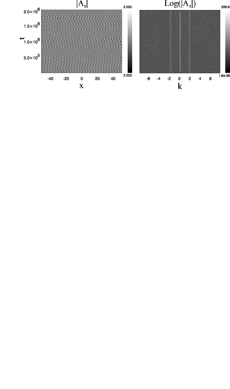
FIG. 5.: Numerical simulation with $E/E_{t}=0.9999$ and $L=103.057$, showing the space-time evolution of $|A_{1}|$ in the near field (left) and far field (right). A similar behavior is seen for the SH.

IV Correlations, photon interaction and pattern formation

Our general objective is the investigation of the spatial intra-cavity field correlations emerging in this system as a result of the coupling of FH and SH field through the nonlinearity of the crystal, and the implications of the spatial instability on these correlations. This study has a two-fold purpose: First, to obtain a precise picture on how pattern formation occurs in cavity SHG. In particular, we will aim at identifying the relevant mechanisms, in terms of elementary three-wave processes that are important for the understanding of the intra-cavity field dynamics. Secondly, it will be interesting to investigate whether these correlations are the manifestation of nonclassical states of the fields. Such states are identified by investigating the statistics of the intra-cavity intensities, looking in particular for possible sub-Poissonian features [31].

A Photon interaction

We will start by investigating the equal time correlations between intensity fluctuations at different points in the far field. The intensity of each field being directly proportional to the number of photons in the corresponding mode, we can relate the intensity fluctuations to the creation or destruction of photons. The idea is that the way these fluctuations are correlated gives information about the microscopic mechanisms that take place in the cavity and, ultimately, that are involved in the pattern formation process. Generally speaking, a positive correlation tells us that there should exist a coherent mechanism that creates simultaneously the corresponding photons. The following normalized correlations are considered

$$C_{ij}^{n}(k,k^{\prime})=\frac{\langle\delta\hat{N}_{i}(k,t)\delta\hat{N}_{j}(k^{\prime},t)\rangle}{\sqrt{\langle\delta\hat{N}_{i}(k,t)^{2}\rangle\langle\delta\hat{N}_{j}(k^{\prime},t)^{2}\rangle}},$$ (73)

where the superscript $n$ denotes normalization. The intensity fluctuations are given by $\delta\hat{N}_{j}(k,t)=\hat{N}_{j}(k,t)-\langle\hat{N}_{j}(k,t)\rangle$, which involves the photon number operator $\hat{N}_{j}(k,t)=\hat{A}_{j}^{\dagger}(k,t)\hat{A}_{j}(k,t)$. The brackets denote quantum mechanical averages (expectations) of the operators, which in our approach based on numerical simulations of equivalent c-numbers will be translated into an average over time. The normalization of the correlations implies that $C_{ij}^{n}(k,k^{\prime})=1$ for perfectly correlated fluctuations, whereas $C_{ij}^{n}(k,k^{\prime})=-1$ will be the signature of perfect anti-correlation between the intensity fluctuations. As usual, the absence of any correlation will translate into a vanishing correlation function $C_{ij}^{n}(k,k^{\prime})=0$. In the following we will refer to $C^{n}_{11}(k,k^{\prime})$ and $C^{n}_{22}(k,k^{\prime})$ as self-correlations (between different modes of a given field) and to $C^{n}_{12}(k,k^{\prime})$ as cross-correlations (between modes in different fields).

As a guideline for the investigation of the properties of these correlation functions, the first step consists in identifying the basic photon processes when the system is taken close to a transverse instability. These photon processes must obey the standard energy and momentum conservation laws. Whereas the former merely implies that each elementary process must connect one SH photon with two FH photons, the latter will translate into a condition on the transverse wave numbers. Keeping in mind that the cavity is pumped with an homogeneous field at the frequency $\omega$, the first process to consider consists in two homogeneous FH photons, $[\omega](k=0)\equiv[\omega](0)$ combining to give one homogeneous SH photon, $[2\omega](0)$, what will be written as $[\omega](0)+[\omega](0)\rightarrow[2\omega](0)$. This is encoded in the Hamiltonian term $\hat{A}_{1}^{2}\hat{A}_{2}^{\dagger}$ in Eq. (5). The inverse process, which corresponds to the degenerate OPO process, also takes place in the system, as shown by the presence of the term $(\hat{A}_{1}^{\dagger})^{2}\hat{A}_{2}$ in Eq. (5). Elaborating on these considerations we propose the scheme in Fig. 6 as the simplest way of obtaining a pattern in both fields.

• The first step is the basic SHG channel where two homogeneous FH photons give a SH photon and vice versa, i.e. the channel $[\omega](0)+[\omega](0)\leftrightarrow[2\omega](0)$. It is important to realize that fluctuations around the steady state are considered, hence it is not considered how the FH photons combine to give the steady state SH photons via the channel above, but rather how the fluctuations invoke the channel beyond this.

• The second step is the down-conversion of a SH photon into two FH photons. Momentum conservation in the process implies that the two FH photons have the same value of the transverse wave number but with opposite signs. These are called twin photons since an emission of a $[\omega](+k^{\prime})$ photon must be accompanied by an emission of a $[\omega](-k^{\prime})$ photon, and they therefore show a high degree of correlation. This channel written as $[2\omega](0)\leftrightarrow[\omega](-k^{\prime})+[\omega](+k^{\prime})$ generates off-axis FH photons.

• Off-axis SH photons are obtained by combining the created off-axis FH photon from step 2) with a photon from the homogeneous background to give a SH photon, which by momentum conservation must have the same wave number as the off-axis FH photon. This channel can be written as $[\omega](0)+[\omega](+k^{\prime})\leftrightarrow[2\omega](+k^{\prime})$.

FIG. 6.: The basic picture of pattern formation on a microscopic level through SHG. The single arrows ($\rightarrow$) symbolize FH photons, while double arrows ($\Rightarrow$) symbolize SH photons. The dashed arrows are photons from the homogeneous background.

Of course, these are not the only three-wave processes which are kinematically allowed in the nonlinear crystal, since the interaction Hamiltonian (5) induces any process of the form $[\omega](k^{\prime})+[\omega](k^{\prime\prime})\leftrightarrow[2\omega](k^{\prime}+k^{\prime\prime})$, with arbitrary wave numbers $k^{\prime}$ and $k^{\prime\prime}$. In fact, the basic scheme we propose in Fig. 6 only takes into account those three-wave processes which involve at least one photon of the homogeneous background fields. Empirically, this choice is motivated by the observation that below the threshold these are the only field modes that are macroscopically populated, so that any process involving them should be stimulated in analogy to what occurs in standard stimulated emission. Formally, the selection of these particular elementary processes corresponds precisely to the approximation made by linearizing the field equations around the steady state solution. As can easily be checked, the full equations for the far field fluctuations contain additional terms quadratic in the fluctuation amplitudes, which indeed account for other three-wave processes. Linearizing we are left with Eq. (63), which only take into account the processes represented by step 2) and step 3). These processes translate into nondiagonal elements of the matrix ${\bf M}(k)$ of the linear system, and as a consequence, for any value of $k$, the time evolution of the four amplitudes $\beta_{1}(k,t)$, $\beta_{1}(-k,t)$, $\beta_{2}(k,t)$ and $\beta_{2}(-k,t)$ will be coupled. This coupling is expected to translate into correlations between the intensity fluctuations $\delta I_{1}(k)$, $\delta I_{1}(-k)$, $\delta I_{2}(k)$, $\delta I_{2}(-k)$.

This preliminary observation already allows to give a more explicit interpretation of the basic scheme of Fig. 6. Splitting the dynamics of the intra-cavity fields into independent elementary steps, as suggested in the discussion of Fig. 6, would not explain any correlations either between $[\omega](k^{\prime})$ and $[2\omega](-k^{\prime})$ nor between $[2\omega](k^{\prime})$ and $[2\omega](-k^{\prime})$. Hence the inspection of the linearized equations shows that the interpretation of Fig. 6 in terms of a cascade is too naive. Instead, we have to understand step 2) and 3) as two coherent, joint processes, which generate simultaneously correlations between the 4 modes $[\omega](k^{\prime})$, $[\omega](-k^{\prime})$, $[2\omega](k^{\prime})$ and $[2\omega](-k^{\prime})$. Finally, it is important to stress that the linearized analysis does not predict any correlation between intensity fluctuations in field modes with wave numbers of different modulus. Mathematically, this is due to the fact that in the linear approximation all correlation functions (73) have the structure

$$C_{ij}(k,k^{\prime})=C_{ij}^{(-)}(k)\delta^{2}(k-k^{\prime})+C_{ij}^{(+)}(k)\delta^{2}(k+k^{\prime}),$$ (74)

as will be shown in the next section. Close enough to threshold, however, this will not be true any more because of the emergence of additional correlations of nonlinear nature.

Let us finally briefly address the fundamental difference between OPO and SHG: Whereas in SHG, the two fields ${\mathcal{A}}_{1}$ and ${\mathcal{A}}_{2}$ are always nonzero regardless of the pump level, in the OPO case below the oscillation threshold ${\mathcal{A}}_{2}$ is fixed by the pump and ${\mathcal{A}}_{1}=0$. Considering the scheme presented in Fig. 6, the vanishing of ${\mathcal{A}}_{1}$ implies that there is no macroscopic population of the mode $[\omega](0)$ and therefore, step 3) of Fig. 6 is not present. The route to pattern formation simply consists of step 2) in Fig. 6, generating correlations between $\delta\hat{N}_{1}(k,t)$ and $\delta\hat{N}_{1}(-k,t)$. Mathematically, the consequence for the stability of the homogeneous solution is that the two equations (III) effectively decouple and that only the FH becomes unstable at the threshold.

B Correlations below shot-noise

Once correlations between intensity fluctuations are identified, it is interesting to investigate if they are connected to nonclassical states of the intra-cavity fields. A coherent field obeys Poissonian photon statistics, which implies that the variance and the mean of the photon number operator $\hat{N}$ are equal. Let us consider the photon number operators associated with the sum and difference of the intensities at different far-field points $\hat{N}_{i}(k)\pm\hat{N}_{j}(k^{\prime})$, where $\hat{N}_{i}(k)=\hat{a}_{i}^{\dagger}(k)\hat{a}_{i}(k)$ and $\hat{N}_{j}(k)=\hat{a}_{j}^{\dagger}(k)\hat{a}_{j}(k)$ are the number operators of two states $\hat{a}_{i}(k,t)$ and $\hat{a}_{j}(k,t)$. Since we will consider equal time correlation functions in the steady state of the system, from now on we will drop the time argument of the field operators. Taking out the special case $i=j$ and $k^{\prime}=k$ which will be treated separately, the variance expressed in normal order (indicated by dots) reads

$${\mathrm{V}ar}(\hat{N}_{i}(k) \pm\hat{N}_{j}(k^{\prime}))=:\!{\mathrm{V}ar}(\hat{N}_{i}(k)\pm\hat{N}_{j}(k^{\prime}))\!:$$ (75)

$$+\langle:\!\hat{N}_{i}(k)\!:\rangle[\hat{a}_{i}(k),\hat{a}_{i}^{\dagger}(k)]$$ (76)

$$+\langle:\!\hat{N}_{j}(k^{\prime})\!:\rangle[\hat{a}_{j}(k^{\prime}),\hat{a}_{j}^{\dagger}(k^{\prime})],$$ (77)

where ${\mathrm{V}ar}(X)\equiv\langle X^{2}\rangle-\langle X\rangle^{2}$. For a coherent state, the normal ordered variance vanishes, and the mean, given by last two terms in (77), represents the shot noise level for the considered quantity

$$S.N.=\langle:\!\hat{N}_{i}(k)\!:\rangle[\hat{a}_{i}(k),\hat{a}_{i}^{\dagger}(k)]+\langle:\!\hat{N}_{j}(k^{\prime})\!:\rangle[\hat{a}_{j}(k^{\prime}),\hat{a}_{j}^{\dagger}(k^{\prime})].$$ (78)

If the normal ordered variance becomes negative

$$:\!{\mathrm{V}ar}(\hat{N}_{i}\pm\hat{N}_{j})\!:<0,$$ (79)

the variance becomes less than the mean, indicating sub-Poissonian behavior. Such a nonclassical state is identified when the correlation normalized to the shot-noise level, defined as

$$C_{ij}^{(\pm)}(k,k^{\prime})\equiv$$ (80)

$$\frac{:\!{\mathrm{V}ar}[\hat{N}_{i}(k)\pm\hat{N}_{j}(k^{\prime})]\!:}{\langle:\!\hat{N}_{i}(k)\!:\rangle[\hat{a}_{i}(k),\hat{a}_{i}^{\dagger}(k)]+\langle:\!\hat{N}_{j}(k^{\prime})\!:\rangle[\hat{a}_{j}(k^{\prime}),\hat{a}_{j}^{\dagger}(k^{\prime})]}+1,$$ (81)

is such that $C_{ij}^{(\pm)}(k,k^{\prime})<1$. The computation of this quantity requires to write the normal ordered quantities appearing in (81) in terms of anti-normal ordered quantities, since these are the quantities that are computed as averages in our Langevin equations associated with the Q representation. Using the identities

$$\vdots\hat{N}_{i}(k)\vdots = \hat{a}_{i}(k)\hat{a}^{\dagger}_{i}(k)=:\!\hat{N}_{i}(k)\!:+[\hat{a}_{i}(k),\hat{a}^{\dagger}_{i}(k)],$$ (83)

$$\vdots\hat{N}^{2}_{i}(k)\vdots = \hat{a}_{i}(k)\hat{a}_{i}(k)\hat{a}^{\dagger}_{i}(k)\hat{a}^{\dagger}_{i}(k)$$ (84)

$$= :\!\hat{N}_{i}(k)^{2}\!:+4:\!\hat{N}_{i}(k)\!:[\hat{a}_{i}(k),\hat{a}^{\dagger}_{i}(k)]$$ (86)

$$+2[\hat{a}_{i}(k),\hat{a}^{\dagger}_{i}(k)]^{2}$$

with three dots indicating anti-normal ordering, Eq. (81) reads, when expressed in terms of anti-normal ordered quantities

$$C_{ij}^{(\pm)}(k,k^{\prime})=\frac{\vdots{\mathrm{V}ar}[\hat{N}_{i}(k)\pm\hat{N}_{j}(k^{\prime})]\vdots-\langle\vdots\hat{N}_{i}(k)\vdots\rangle[\hat{a}_{i}(k),\hat{a}^{\dagger}_{i}(k)]-\langle\vdots\hat{N}_{j}(k^{\prime})\vdots\rangle[\hat{a}_{j}(k^{\prime}),\hat{a}^{\dagger}_{j}(k^{\prime})]}{\langle\vdots\hat{N}_{i}(k)\vdots\rangle[\hat{a}_{i}(k),\hat{a}^{\dagger}_{i}(k)]+\langle\vdots\hat{N}_{j}(k^{\prime})\vdots\rangle[\hat{a}_{j}(k^{\prime}),\hat{a}^{\dagger}_{j}(k^{\prime})]-[\hat{a}_{i}(k),\hat{a}^{\dagger}_{i}(k)]^{2}-[\hat{a}_{j}(k^{\prime}),\hat{a}^{\dagger}_{j}(k^{\prime})]^{2}}.$$ (87)

Then e.g. the normalized correlation ${\mathrm{V}ar}[\hat{N}_{1}(k)\pm\hat{N}_{1}(-k)]/{S.N.}$ may be found by setting $i=j=1$ and $k^{\prime}=-k$. Equation (87) is valid for $k,k^{\prime}\neq 0$, while the special case $k=0$ will be addressed in the specific cases.

V Linearized calculations below threshold

Below threshold, the linear approximation scheme allows to derive semi-analytical expressions for the correlation functions defined in the previous section. These may be expressed in terms of the auxiliary correlation function

$$C_{ij}^{Q}(k,k^{\prime}) = {\langle\vdots\delta\hat{N}_{i}(k,t)\delta\hat{N}_{j}(k^{\prime},t)\vdots\rangle},\quad i,j=1,2$$ (88)

$$= {\langle|A_{i}(k,t)|^{2}|A_{j}(k^{\prime},t)|^{2}\rangle}$$ (90)

$$-{\langle|A_{i}(k,t)|^{2}\rangle\langle|A_{j}(k^{\prime},t)|^{2}\rangle},$$

where the superscript Q indicates that the average is done with the Q representation, corresponding to anti-normal ordered quantities, as indicated in the first line of (90).

The starting point of our analysis is the set of linearized Langevin equations (63) which have the exact solutions

$$\left(\begin{array}[]{c}\beta_{1}(k,t)\\ \beta_{1}^{*}(-k,t)\\ \beta_{2}(k,t)\\ \beta_{2}^{*}(-k,t)\end{array}\right)=e^{{\mathbf{M}}(k)t}\left(\begin{array}[]{c}\beta_{1}(k,0)\\ \beta_{1}^{*}(-k,0)\\ \beta_{2}(k,0)\\ \beta_{2}^{*}(-k,0)\end{array}\right)$$ (99)

$$+\sqrt{\frac{2}{n_{th}}}e^{{\mathbf{M}}(k)t}\int_{0}^{t}dt^{\prime}e^{-{\mathbf{M}}(k)t^{\prime}}\left(\begin{array}[]{c}\eta_{1}(k,t^{\prime})\\ \eta_{1}^{*}(-k,t^{\prime})\\ \sqrt{\gamma}\eta_{2}(k,t^{\prime})\\ \sqrt{\gamma}\eta_{2}^{*}(-k,t^{\prime})\end{array}\right).$$ (104)

The first term in Eq. (104) describes how the intra-cavity fields with arbitrary initial conditions relax to the steady state solution and it does not contribute to the steady state correlations. The second term in Eq. (104) gives the response of the intra-cavity fields to the vacuum fluctuations entering the cavity through the partially transparent input mirror. Starting from Eq. (104), it is possible to derive semi-analytical expressions for the correlations (90)

$$C^{Q}_{ij}(k,k^{\prime}) = \langle|\beta_{i}(k,t)|^{2}|\beta_{j}(k^{\prime},t)|^{2}\rangle$$ (105)

$$- \langle|\beta_{i}(k,t)|^{2}\rangle\langle|\beta_{j}(k^{\prime},t)|^{2}\rangle$$ (106)

$$+ 2{\mathrm{R}e}\big{\{}{\mathcal{A}}_{i}^{*}{\mathcal{A}}_{j}\langle\beta_{i}(k,t)\beta^{*}_{j}(k^{\prime},t)\rangle$$ (108)

$$+{\mathcal{A}}_{i}^{*}{\mathcal{A}}_{j}^{*}\langle\beta_{i}(k,t)\beta_{j}(k^{\prime},t)\rangle\big{\}}\delta(k)\delta(k^{\prime}),$$

where ${\mathrm{R}e}\{\cdot\}$ denotes the real part. Whereas the first two terms in the right-hand side (r.h.s.) of Eq. (108) measure the correlations in the intensities of the fluctuations, the last two terms can be traced back to interferences between the fluctuations and the homogeneous component of each field. Since these interferences only contribute to the equal time correlations when $k=k^{\prime}=0$, we will first concentrate on $k,k^{\prime}\neq 0$ and come back later to this special case. Henceforth, unless otherwise specified we consider the case $k,k^{\prime}\neq 0$.

The Gaussian character of the fluctuations in this linearized Langevin model allows to factorize (108) in terms of second order moments of the field fluctuations

$$C^{Q}_{ij}(k,k^{\prime})=|\langle\beta_{i}(k,t)\beta^{*}_{j}(k^{\prime},t)\rangle|^{2}+|\langle\beta_{i}(k,t)\beta_{j}(k^{\prime},t)\rangle|^{2}.$$ (109)

The field correlations $\langle\beta_{i}(k,t)\beta^{*}_{j}(k^{\prime},t)\rangle$ and $\langle\beta_{i}(k,t)\beta_{j}(k^{\prime},t)\rangle$ can be best evaluated for the solution Eq. (104) if we introduce the set of eigenvectors $\{{\mathbf{v}}^{(l)}(k)\}_{l=1,...,4}$ of the matrix ${\mathbf{M}}(k)$, defined through:

$${\mathbf{M}}(k){\mathbf{v}}^{(l)}(k)=\lambda^{(l)}(k){\mathbf{v}}^{(l)}(k).$$ (110)

An arbitrary $4$-component vector ${\mathbf{w}}$ can be decomposed on this basis

$${\mathbf{w}}(k)=\left(\begin{array}[]{c}w_{1}(k)\\ w_{2}(k)\\ w_{3}(k)\\ w_{4}(k)\end{array}\right)=\sum_{l=1}^{4}w^{(l)}(k){\mathbf{v}}^{(l)}(k),$$ (111)

and its components $w^{(l)}$ in the new basis are calculated via the linear transformation

$$w^{(l)}(k)=\sum_{m=1}^{4}T_{lm}(k)w_{m}(k).$$ (112)

This involves a $4\times 4$ matrix $T_{lm}(k)$ calculated as ${\mathbf{T}}(k)={\mathbf{V}}(k)^{-1}$ with $V_{lm}(k)=v^{(m)}_{l}(k)$. Decomposing now the noise vector appearing on the r.h.s. of Eq. (104) on this basis

$$\left(\begin{array}[]{c}\eta_{1}(k,t^{\prime})\\ \eta_{1}^{*}(-k,t^{\prime})\\ \sqrt{\gamma}\eta_{2}(k,t^{\prime})\\ \sqrt{\gamma}\eta_{2}^{*}(-k,t^{\prime})\end{array}\right)=\sum_{l=1}^{4}\eta^{(l)}(k,t^{\prime}){\mathbf{v}}^{(l)}(k),$$ (113)

allows to rewrite Eq. (104) in the large time limit as

$$\left(\begin{array}[]{c}\beta_{1}(k,t)\\ \beta_{1}^{*}(-k,t)\\ \beta_{2}(k,t)\\ \beta_{2}^{*}(-k,t)\end{array}\right) =\sqrt{\frac{2}{n_{th}}}\int_{0}^{t}dt^{\prime}$$ (119)

$$\times\sum_{l=1}^{4}e^{{\lambda}^{(l)}(k)(t-t^{\prime})}\eta^{(l)}(k,t^{\prime}){\mathbf{v}}^{(l)}(k).$$

The needed field correlations are given as

$$\langle\beta_{i}(k,t)\beta_{j}^{*}(k^{\prime},t)\rangle = \frac{2}{n_{th}}\int_{0}^{t}dt^{\prime}\int_{0}^{t}dt^{\prime\prime}\sum_{l,m=1}^{4}v_{2i-1}^{(l)}(k){v_{2j-1}^{(m)}}^{*}(k^{\prime})e^{{\lambda}^{(l)}(k)(t-t^{\prime})}e^{{\lambda^{(m)}}^{*}(k^{\prime})(t-t^{\prime\prime})}\langle\eta^{(l)}(k,t^{\prime}){\eta^{(m)}}^{*}(k^{\prime},t^{\prime\prime})\rangle,$$ (121)

$$\langle\beta_{i}(k,t)\beta_{j}(k^{\prime},t)\rangle = \frac{2}{n_{th}}\int_{0}^{t}dt^{\prime}\int_{0}^{t}dt^{\prime\prime}\sum_{l,m=1}^{4}v_{2i-1}^{(l)}(k)v_{2j-1}^{(m)}(k^{\prime})e^{{\lambda}^{(l)}(k)(t-t^{\prime})}e^{{\lambda}^{(m)}(k^{\prime})(t-t^{\prime\prime})}\langle\eta^{(l)}(k,t^{\prime})\eta^{(m)}(k^{\prime},t^{\prime\prime})\rangle.$$ (122)

The noise correlations in the new basis $\langle\eta^{(l)}(k,t^{\prime}){\eta^{(m)}}^{*}(k^{\prime},t^{\prime\prime})\rangle$ and $\langle\eta^{(l)}(k,t^{\prime})\eta^{(m)}(k^{\prime},t^{\prime\prime})\rangle$ are

$$\langle\eta^{(l)}(k,t^{\prime}){\eta^{(m)}}^{*}(k^{\prime},t^{\prime\prime})\rangle = A_{lm}(k)\delta(k-k^{\prime})\delta(t^{\prime}-t^{\prime\prime}),$$ (124)

$$\langle\eta^{(l)}(k,t^{\prime})\eta^{(m)}(k^{\prime},t^{\prime\prime})\rangle = B_{lm}(k)\delta(k+k^{\prime})\delta(t^{\prime}-t^{\prime\prime}).$$ (125)

where the matrix elements of the $4\times 4$ matrices ${\mathbf{A}}(k)$ and ${\mathbf{B}}(k)$ can easily be evaluated in terms of the matrix elements $T_{lm}\equiv T_{lm}(k)$ as

$$A_{lm}(k)= T_{l1}T^{*}_{m1}-\frac{{\mathcal{A}}_{2}}{2}T_{l1}T^{*}_{m2}+T_{l2}T^{*}_{m2}$$ (128)

$$-\frac{{\mathcal{A}}^{*}_{2}}{2}T_{l2}T^{*}_{m1}+\gamma T_{l3}T^{*}_{m3}+\gamma T_{l4}T^{*}_{m4},$$

$$B_{lm}(k)= T_{l1}T_{m2}-\frac{{\mathcal{A}}_{2}}{2}T_{l1}T_{m1}+T_{l2}T_{m1}$$ (130)

$$-\frac{{\mathcal{A}}^{*}_{2}}{2}T_{l2}T_{m2}+\gamma T_{l3}T_{m4}+\gamma T_{l4}T_{m3}.$$

Inserting Eqs. (V) in Eqs. (V) we can easily carry out the time integration, and neglecting transient contributions, we end up with the following expressions

$$\lim_{t\to\infty}\langle\beta_{i}(k,t)\beta^{*}_{j}(k^{\prime},t)\rangle = \frac{2}{n_{th}}G_{ij}^{(-)}(k)\delta(k-k^{\prime}),$$ (132)

$$\lim_{t\to\infty}\langle\beta_{i}(k,t)\beta_{j}(k^{\prime},t)\rangle = \frac{2}{n_{th}}G_{ij}^{(+)}(k)\delta(k+k^{\prime}).$$ (133)

with

$$G_{ij}^{(-)}(k)=\sum_{l=1}^{4}\sum_{m=1}^{4}A_{lm}(k)\frac{v_{2i-1}^{(l)}(k){v_{2j-1}^{(m)}}^{*}(k)}{-(\lambda^{(l)}(k)+{\lambda^{(m)}}^{*}(k))},$$ (135)

$$G_{ij}^{(+)}(k)=\sum_{l=1}^{4}\sum_{m=1}^{4}B_{lm}(k)\frac{v_{2i-1}^{(l)}(k)v_{2j-1}^{(m)}(k)}{-(\lambda^{(l)}(k)+\lambda^{(m)}(k))}.$$ (136)

In terms of $G_{ij}^{(-)}(k)$ and $G_{ij}^{(+)}(k)$, Eq. (109) is given by

$$C^{Q}_{ij}(k,k^{\prime})= \frac{4}{n_{th}^{2}}\big{[}|G_{ij}^{(-)}(k)|^{2}\delta^{2}(k-k^{\prime})$$ (138)

$$+|G_{ij}^{(+)}(k)|^{2}\delta^{2}(k+k^{\prime})\big{]}.$$

A Intensity fluctuation correlations

It is now easy to compute the normalized correlation function Eq. (73). This involves taking into account the commutation relation Eq. (1) which reads

$$\big{[}{\hat{A}_{i}}(k,t),{\hat{A}_{j}}^{\dagger}(k^{\prime},t)\big{]}=\delta_{ij}\frac{1}{n_{th}}\delta(k-k^{\prime}),$$ (139)

after rescaling space and time according to Eq. (23) and the operators similar to the c-number fields in Eq. (25). We finally find

$$C^{n}_{ij}(k,k^{\prime})= \frac{|G_{ij}^{(-)}(k)|^{2}}{\sqrt{\eta_{i}(k)}\sqrt{\eta_{j}(k)}}\frac{\delta(k-k^{\prime})^{2}}{\delta(0)^{2}}$$ (141)

$$+\frac{|G_{ij}^{(+)}(k)|^{2}}{\sqrt{\eta_{i}(k)}\sqrt{\eta_{j}(k)}}\frac{\delta(k+k^{\prime})^{2}}{\delta(0)^{2}},$$

with $\eta_{j}(k)=G_{jj}^{(-)}(k)(G_{jj}^{(-)}(k)-1/2)$, the $-1/2$ in the parenthesis reflecting the conversion from anti-normal to direct ordering. Unlike the mathematical expression (141) derived for an ideally infinite system, the correlation functions determined from the simulations will have peaks of a finite width, which will be determined by the discretization in $k$-space used in the numerical codes, i.e. the inverse of the total length of the system. This difference, however, will not alter the only relevant information, which is the height of each of these peaks. In fact, the quantities

$$C^{n}_{jj}(k,-k) = \frac{|G_{jj}^{(+)}(k)|^{2}}{{\eta_{j}(k)}}$$ (143)

$$C^{n}_{12}(k,\pm k) = \frac{|G_{12}^{(\mp)}(k)|^{2}}{\sqrt{\eta_{1}(k)}\sqrt{\eta_{2}(k)}},$$ (144)

characterize the strength of the correlations between the modes $[\omega](k)$ and $[\omega](-k)$, $[2\omega](k)$ and $[2\omega](-k)$, $[\omega](k)$ and $[2\omega](k)$, and $[\omega](k)$ and $[2\omega](-k)$ respectively. One easily checks that $C^{n}_{ii}(k,k)=1$, as a result of an autocorrelation.

All the expressions derived so far are only valid for nonvanishing transverse wave numbers. At $k=k^{\prime}=0$, we already observed that there are extra contributions to the equal time correlation function, as expressed by Eq. (108). Furthermore, in the framework of an expansion in the small parameter $\sqrt{2/n_{th}}$, it is obvious that these extra terms even dominate, since they scale with $|\beta_{i}(k,t)|^{2}\sim 2/n_{th}$, whereas the contributions on the first line of Eq. (108) scales with $|\beta_{i}(k,t)|^{4}\sim(2/n_{th})^{2}$. Hence, in the leading order, the correlation function at $k=k^{\prime}=0$ is given by

$$C_{12}^{Q}(k,k^{\prime}) \big{|}_{k=k^{\prime}=0}=\frac{2\delta(0)}{n_{th}}2{\mathrm{R}e}\Big{(}{\mathcal{A}}_{1}^{*}{\mathcal{A}}_{2}G_{12}^{(-)}(0)$$ (146)

$$+{\mathcal{A}}_{1}^{*}{\mathcal{A}}_{2}^{*}G_{12}^{(+)}(0)\Big{)}\delta(k)\delta(k^{\prime})\big{|}_{k=k^{\prime}=0}.$$

Similar calculations as before allow us to derive the following expression for the value of the normalized cross-correlation at $k=k^{\prime}=0$

$$C^{n}_{12}(0,0)=\frac{{\mathrm{R}e}\left({\mathcal{A}}_{1}^{*}{\mathcal{A}}_{2}G_{12}^{(-)}(0)+{\mathcal{A}}_{1}^{*}{\mathcal{A}}_{2}^{*}G_{12}^{(+)}(0)\right)}{\sqrt{\zeta_{1}}\sqrt{\zeta_{2}}},$$ (147)

where $\zeta_{j}=|{\mathcal{A}}_{j}|^{2}(G_{jj}^{(-)}(0)-1/4)+{\mathrm{R}e}\{{{\mathcal{A}}_{j}^{*}}^{2}G_{jj}^{(+)}(0)\}$.

B Nonclassical photon number variances

The photon number variances considered in Sec. IV B can be calculated in terms of the auxiliary functions $G_{ij}^{(-)}(k)$ and $G_{ij}^{(+)}(k)$ as well. The anti-normal ordered quantities in Eq. (87) can be directly calculated by averages in the Langevin equation, so below threshold the anti-normal ordered variance is for $k\neq 0$

$$\vdots{\mathrm{V}ar}[\hat{N}_{i}(k)\pm\hat{N}_{j}(-k)]\vdots={\mathrm{V}ar}[|\beta_{i}(k,t)|^{2}\pm|\beta_{j}(-k,t)|^{2}].$$ (148)

Using the commutation relations (139), the commutators in Eq. (87) are $[a_{j}(k),a^{\dagger}_{j}(k)]=\delta(0)/n_{th}$, and the normalized self-correlations takes the form

$$C_{jj}^{(\pm)}(k,-k)=\frac{2\left(|G_{jj}^{(-)}(k)|^{2}\pm|G_{jj}^{(+)}(k)|^{2}\right)-G_{jj}^{(-)}(k)}{G_{jj}^{(-)}(k)-1/2}.$$ (149)

Similarly, the cross-correlations are

$$C_{12}^{(\pm)}(k,\nu k)=\frac{2\left(\sum_{j}|G_{jj}^{(-)}(k)|^{2}\pm 2|G_{12}^{(-\nu)}(k)|^{2}\right)-\sum_{j}G_{jj}^{(-)}(k)}{\sum_{j}G_{jj}^{(-)}(k)-1},\quad\nu=+1,-1$$ (150)

When $k=k^{\prime}=0$ Eq. (148) is no longer valid. Instead, following the procedure outlined for the normalized correlations we have to the leading order $O(n_{th}^{-1})$

$$C_{12}^{(\pm)}(0,0)=4\frac{{\mathrm{R}e}\left[\sum_{j}{{\mathcal{A}}_{j}^{*}}^{2}G_{jj}^{(+)}(0)\pm 2{\mathcal{A}}_{1}^{*}\left({\mathcal{A}}_{2}^{*}G_{12}^{(+)}(0)+{\mathcal{A}}_{2}G_{12}^{(-)}(0)\right)\right]+\sum_{j}|{\mathcal{A}}_{j}|^{2}G_{jj}^{(-)}(0)}{\sum_{j}|{\mathcal{A}}_{j}|^{2}}-1.$$ (151)

The self-correlations become

$$C_{jj}^{(-)}(0,0) = 0,$$ (153)

$$C_{jj}^{(+)}(0,0) = 4{\mathrm{R}e}\left[e^{-i2\phi_{A_{j}}}G_{jj}^{(+)}(0)\right]+4G_{jj}^{(-)}(0)-1.$$ (154)

where $\phi_{A_{j}}$ is the phase of ${\mathcal{A}}_{j}$. Note that $C_{jj}^{(+)}(0,0)$ is actually ${\mathrm{V}ar}[\hat{N}_{j}(0)]$ normalized to shot-noise. The result of Eq. (153) is simply because the correlation $C_{jj}^{(-)}(k,k^{\prime})$ amounts to calculating the variance of zero for $k=k^{\prime}=0$.

FIG. 7.: The linear self-correlations a) $C^{n}_{11}(k,-k)$, b) $C^{n}_{22}(k,-k)$ and linear cross-correlations c) $C^{n}_{12}(k,k)$, d) $C^{n}_{12}(k,-k)$ as function of the transverse wave number for $E/E_{t}=0.99$. The points are numerical results while the lines are analytical results.

VI Correlations below threshold

The linearized results of Sec. V gives an analytical insight to the behaviour below threshold for pattern formation. However, very close to the threshold this linear approximation breaks down because of critical nonlinear fluctuations, and additional contributions may emerge as for example shown in a vector Kerr model by Hoyuelos et al. [32]. Such nonlinear correlations can be calculated through numerical simulations of the full nonlinear evolution equations.

In this section we present numerical results obtained from simulations of the nonlinear equations (II) below threshold, with the parameters discussed in Sec. III. Our numerical results are compared with the analytical results of the previous section, and therefore also serves as a cross-check of our analytical and numerical methods.

A Linear correlations: Analytical and numerical results

We first consider the strength of the correlations between symmetric points in the far fields below the threshold for pattern formation. In Fig. 7, the four quantities defined by Eq. (73) are plotted. The data are obtained from numerical simulations and from the analytical results of Eqs. (V A) and (147). Very good agreement is found between numerics and analytical results.

There are three main features to be considered in the results of Fig. 7. First, all curves present a distinctly peaked behavior around the critical wave number $k_{c}$ for pattern formation, which means that the corresponding modes are more strongly correlated than the modes at any other wave number. Manifestly, this behavior is connected with the pattern formation mechanism and is closely related to the phenomenon of quantum images [10]. Secondly, we also note that in all four plots the correlations show a jump at $k=0$. In a) and b) it is the trivial manifestation of an auto-correlation, since for $k=0$, $k$ and $-k$ coincide, while in c) and d) the jump is due to the extra interferences with the homogeneous background fields as predicted from Eq. (147). Finally, we observe that the peaks localized around $k_{c}$ are superimposed onto smooth correlation profiles.

The strong correlations appearing between the modes associated with wave numbers around $k_{c}$ indicate a strongly synchronized emission of photons in the modes $[\omega](+k)$, $[\omega](-k)$ and $[2\omega](+k)$, $[2\omega](-k)$. This behavior reflects the direction of instability of the system. As a matter-of-fact, regardless that all transverse modes of both fields are equally excited by the vacuum fluctuations entering the cavity, the fluctuations of the intra-cavity field modes around the critical wave vector will be less damped than the fluctuations in the other modes. The closer to the threshold, the more the behavior of the intra-cavity fields will be dominated by the mode that becomes unstable at the threshold and gives rise to the pattern. In the 4-dimensional phase space spanned by the fluctuation amplitudes $\{\beta_{1}(k,t),\beta_{1}^{*}(-k,t),\beta_{2}(k,t),\beta_{2}^{*}(-k,t)\}$, this mode is characterized by a vector with a given direction. What we learn from the correlation functions is that the emerging instability results in an almost perfectly synchronized emission of photons in the modes $[\omega](+k)$, $[\omega](-k)$ and $[2\omega](+k)$, $[2\omega](-k)$.

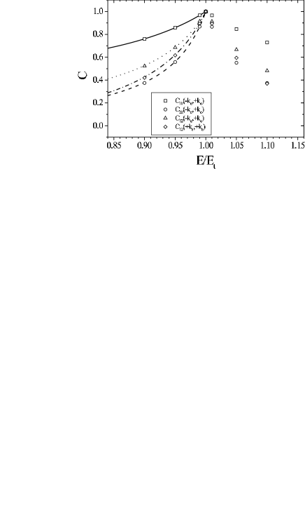
FIG. 8.: The self-correlations $C^{n}_{11}(k_{c},-k_{c})$ (full, squares) and $C^{n}_{22}(k_{c},-k_{c})$ (dashed, circles) and the cross-correlations $C^{n}_{12}(k_{c},-k_{c})$ (dotted, triangles) and $C^{n}_{12}(k_{c},k_{c})$ (dash-dotted, diamonds) as function of the pump normalized to the threshold. The points are numerical results while the lines are analytical results.

The dominance of this particular mode when the threshold is approached is confirmed by the study of the strength of these correlations as a function of the pump. In Fig. 8 we follow the height of the peaks at $k=k_{c}$ of the four linear correlations displayed in Fig. 7, as a function of the pump level $E/E_{t}$. The most immediate observation is that all the correlations become perfect in the limit $E\rightarrow E_{t}$. This asymptotic behavior can be understood from the linearized fluctuation analysis presented in Sec. V. It is enough to observe that Eqs. (V) involve the inverse of the real part of the eigenvalues of the linear system (63). The dominance at the threshold of the undamped eigenmode of the linear system (63) emerges from the fact that here the real part of the associated eigenvalue precisely goes to zero. Thus, the decrease in the correlations as we move away from threshold can be seen as the result of the coexistence of different eigenmodes. Physically the emergence of these correlations is much less intuitive than the ones in an OPO. As a matter-of-fact, in the OPO below the threshold momentum conservation is enough to predict the existence of correlations between the fluctuations in the modes $[\omega](+k)$ and $[\omega](-k)$. In the presence of the 4-mode interaction of SHG, the momentum conservation gives a global condition involving all four beams (at $[\omega](+k)$, $[\omega](-k)$ and $[2\omega](+k)$, $[2\omega](-k)$). These correlations in fact arise in connection with the emergence of an instability.

Turning now to the cross-correlation between the homogeneous components of the fields, we observe that $C^{n}_{12}(k=0,k^{\prime}=0)$ in Fig. 7 is negative, reflecting an anticorrelation of the photons associated with the FH and SH homogeneous waves. In other words, the creation of a photon $[2\omega](0)$ implies the destruction of (two) photons $[\omega](0)$ and vice versa. The origin of this correlation is much simpler to understand than the previous one: The two modes $[\omega](0)$ and $[2\omega](0)$ being macroscopically populated, the vacuum fluctuations simply induce transitions between these two modes, according to step 1) in the scheme in Fig. 6. In Fig. 9 we plot this correlation as a function of the pump. Comparing the value of the correlations below and above threshold, we observe that very close to, but below, the threshold, the tendency of the curve is reversed and it anticipates the behavior of the correlation above threshold. These are nonlinear correlation effects that will be discussed in Sec. VI B.

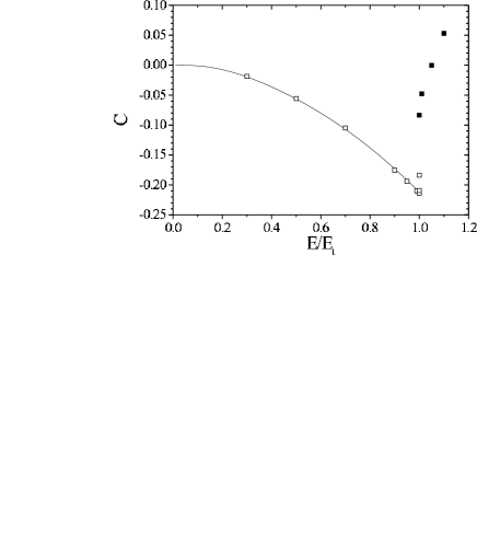
FIG. 9.: The linear cross-correlation $C^{n}_{12}(k=0,k^{\prime}=0)$ as function of the pump normalized to the threshold, comparing numerical results (points) with the analytical result (line). Open (full) symbols are numerics below (above) $E_{t}$.

Finally, we would like to discuss the smooth contributions to the correlations displayed in Fig. 7. We first note that these are not connected with the pattern instability. This was checked by considering very low pump values for which the peaks around $k_{c}$ completely vanish, while the smooth structures of the curves remain. Considering the central region of the curves, roughly for $|k|<k_{c}$, the most striking observation is the absence of correlations between the fluctuations in the modes $[\omega](k)$ and $[2\omega](k)$, whereas $[\omega](k)$ and $[2\omega](-k)$ are correlated, as well as $[2\omega](k)$ with $[2\omega](-k)$. This behavior seems to indicate the existence of a symmetry restoring principle in the dynamics of the intra-cavity fields. As a matter-of-fact, the absence of correlations between $[\omega](k)$ and $[2\omega](k)$ implies that the fluctuations of the numbers of pair productions through step 2) and the fluctuations of the number of conversions $[\omega](k)\to[2\omega](k)$ through step 3) occur independently of each other. However, while step 2) of Fig. 6 conserves the $k\rightarrow-k$ symmetry of the system, step 3) does not. As a consequence, a positive fluctuation in the number of times step 3) occurs ($[\omega](k)+[\omega](0)\rightarrow[2\omega](k)$), automatically implies that there will be less $[\omega](k)$ than $[\omega](-k)$ in the system, and more $[2\omega](k)$ than $[2\omega](-k)$. The correlations observed may indicate that the system will try to restore the $k\rightarrow-k$ symmetry by down-converting $[2\omega](0)\rightarrow[\omega](k)+[\omega](-k)$, producing a surplus of $[\omega](-k)$ which again will produce more $[2\omega](-k)$. These mechanisms seems to fit well with the relative strengths of the correlations observed in the central region of Fig. 7. The strongest is always $C^{n}_{11}(k,-k)$, in agreement with the fact that the twin photon emission is the principal source of correlations in the system. Weaker is the correlation $C_{12}^{n}(k,-k)$ and even weaker $C_{22}^{n}(k,-k)$. This interpretation is consistent with the way the correlations at $k=k_{c}$ depart from the value $1$ at threshold, when the pump is lowered, as displayed in Fig. 8.

FIG. 10.: Photon number variances for $E/E_{t}=0.99$ showing $C_{11}^{(-)}(k,-k)$ (full, diamonds) and $C_{11}^{(+)}(k,-k)$ (dashed, squares). The lines are analytical results while the points are numerical simulations. The shot-noise level $C=1$ is indicated by a thin dotted line.

We now turn our attention to the study of the fluctuations in the sum and difference of the photon numbers at symmetrical points of the far field. We first consider the twin beam photon variances for the FH, $C_{11}^{(\pm)}(k,-k)$ defined in Eq. (81) and shown in Fig. 10. The results are symmetric with respect to the substitution $k\rightarrow-k$, wherefore we plotted this quantity for positive $k$, shifting the origin for better view of the specific behavior at $k=0$. The linearized calculation predicts sub shot-noise statistics in the difference $\hat{N}_{1}(k)-\hat{N}_{1}(-k)$ for all wave numbers. For large wave numbers the analytical result for the correlation approaches the value $1/2$. It is interesting to keep in mind that for the OPO, the same quantity is equal to $1/2$ independently of the wave number [33, 34]. In the SHG case additional processes taking place in the cavity result in a smooth $k$-dependence of $C_{11}^{(-)}(k,-k)$. These characteristics do not depend much on the value of pump, and are not changed significantly even when the pump level is taken beyond threshold, cf. Sec. VII. Therefore, the statistics of the intensity difference is not directly affected by the pattern formation mechanism. A radically different situation occurs for the sum-correlation $C_{11}^{(+)}(k,-k)$, which shows a strong peak around $k=k_{c}$. For the pump value used in Fig. 10 the peaks correspond to a maximum value $C_{11}^{(+)}(k_{c},-k_{c})\simeq 35$. This behavior is connected with the increase of the fluctuations in the modes associated with the pattern instability when the threshold is approached, leading to a large excess noise in the statistics of the intensity of the individual modes $[\omega](k)$ and $[\omega](-k)$. This excess noise in each intensity cancels when the difference $\hat{N}_{1}(k)-\hat{N}_{1}(-k)$ is considered leading to a sub-Poissonian statistics, while it is still present in the sum $\hat{N}_{1}(k)+\hat{N}_{1}(-k)$. For large $k$ the correlation approaches 1.5, coinciding again with the corresponding value for the OPO. Finally, as before, the jumps at $k=0$ are due to contributions from the homogeneous steady states, cf. Eqs. (151)-(151).

FIG. 11.: Photon number variances for $E/E_{t}=0.99$ showing $C_{22}^{(-)}(k,-k)$ (full, diamonds) and $C_{22}^{(+)}(k,-k)$ (dashed, squares).

The corresponding photon number variances $C_{22}^{(\pm)}(k,-k)$ for the SH field are shown in Fig. 11. In contrast to the FH correlations there is almost no sub-shot noise behavior in the difference correlation $C_{22}^{(-)}(k,-k)$. In other words, the SH beams only display very weak nonclassical correlations. As for the FH field, the emerging instability does not influence the noise level in $C_{22}^{(-)}(k,-k)$, but $C_{22}^{(+)}(k,-k)$ displays a large amount of excess noise in the vicinity of $k_{c}$. The asymptotic large $k$ behavior for both correlations $C_{22}^{(-)}(k,-k)$ and $C_{22}^{(+)}(k,-k)$ is analytically found to correspond to the shot-noise limit 1.0.

The cross-correlations $C_{12}^{(-)}(k,k)$ and $C_{12}^{(+)}(k,k)$ are shown in Fig. 12. The linearization approach predicts that these correlations are always above the shot-noise limit. Furthermore, at small wave numbers we note that the variances of the sum and difference coincide. This can only occur when the fluctuations in the individual modes $[\omega](k)$ and $[2\omega](k)$ are uncorrelated, what was indeed observed in Fig. 7. Moreover, both the sum and difference correlations show a large excess noise at $k=k_{c}$, which is slightly weaker for the difference, as the result of a partial noise cancellation.

FIG. 12.: Photon number variances for $E/E_{t}=0.99$ showing $C_{12}^{(-)}(k,k)$ (full, diamonds) and $C_{12}^{(+)}(k,k)$ (dashed, squares).

FIG. 13.: Photon number variances for $E/E_{t}=0.99$ showing $C_{12}^{(-)}(k,-k)$ (full, diamonds) and $C_{12}^{(+)}(k,-k)$ (dashed, squares).

The cross-correlations $C_{12}^{(-)}(k,-k)$ and $C_{12}^{(+)}(k,-k)$ are shown in Fig. 13, and here the difference correlations interestingly go below the shot-noise limit as long as $k$ is not too close to the critical wave number. It is worth pointing out that the difference $\hat{N}_{1}(k)-\hat{N}_{2}(-k)$ shows nonclassical behavior while the difference $\hat{N}_{1}(k)-\hat{N}_{2}(k)$ (shown in Fig. 12) does not. This somehow paradoxical situation is related to what was observed in the normalized correlations where the cross-correlation between $\hat{N}_{1}(k)$ and $\hat{N}_{2}(-k)$ was stronger than the almost vanishing cross-correlation between $\hat{N}_{1}(k)$ and $\hat{N}_{2}(k)$. At $k=k_{c}$ a large amount of excess noise dominates the behavior of both the sum and the difference correlation and the two correlations show a pronounced peak. For large $k$ the correlations approach the shot noise limit, as seen for the other cross-correlations in Fig. 12.

Olsen et al. [35] have investigated the system without spatial coupling corresponding to our results at $k=0$, and they find that, for certain detunings, the variance of the sum of the FH and SH intensities are more strongly quantum correlated than the variance of the individual intensities, due to the anti-correlation between them. ${\mathrm{V}ar}[\hat{N}_{1}(0)]/S.N.$ and ${\mathrm{V}ar}[\hat{N}_{2}(0)]/S.N.$ can be seen from Fig. 10 and 11, respectively, at $k=0$. Both are larger than the ${\mathrm{V}ar}[\hat{N}_{1}(0)+\hat{N}_{2}(0)]/S.N.$ observed in Figs. 12 and 13, so that our results confirm the ones of [35].

B Nonlinear correlations: Numerical results

So far we have only considered the correlations predicted by the linearized equations. In order to go beyond this regime, we use our numerical simulations to search for nonlinear fingerprints in the correlations and in particular for the emergence of new correlations, i.e. $C^{n}_{ij}(k,k^{\prime})$ with $k\neq\pm k^{\prime}$. Of particular interest is to look for correlations between the homogeneous steady states ($k=0$) and the states with $k=\pm k_{c}$, $C^{n}_{ij}(0,\pm k_{c})$. From a technical point of view this task turned out to be difficult because nonlinear contributions to the correlation functions were only observable for pump values extremely close to threshold, in a region where the characteristic time of the dynamics diverges because of critical slowing down. This translates into very long transients and the need of equally long simulations.

We have observed some indication of nonlinear correlations for a pump $E/E_{t}=0.99999$, which became very clear when using $E/E_{t}=0.999999$. For this value of the pump, we show in Fig. 14 our results for $C^{n}_{12}(k,k^{\prime}=0)$ and $C^{n}_{12}(k^{\prime}=0,k)$: these curves put into evidence an anti-correlation between the modes $[\omega](\pm k_{c})$ and $[2\omega](0)$, and between $[2\omega](\pm k_{c})$ and $[\omega](0)$ . They present a very sharp peak structure, with a width determined by the distance between two adjacent points of the discretized $k$-space used for the simulations. This is due to the fact that we now consider the correlation functions at fixed $k^{\prime}$ and let $k$ vary. These correlations are a result of nonlinear amplification of the diverging fluctuations as the threshold is approached. The negative nature of the correlation is connected with the fact that the fields with nonzero average values (here the homogeneous components) act as a ”reservoir” of photons for all processes occurring in the cavity. As we will show later, they are a precursor of the behavior of the correlations above the threshold. The correlations at $k=0$ correspond to the linear correlation shown in Fig. 9. The bottom plot in Fig. 14 shows the nonlinear correlations $C^{n}_{ij}(k=+k_{c},k^{\prime}=0)$ as the threshold is approached. The correlations are nonzero only for $E/E_{t}>0.9999$. As the nonlinear correlations set in the nonlinear channels in step 2) and 3) of Fig. 6 become stronger and this weakens the correlations induced by the channel of step 1), which is exactly what we observed in Fig. 9; $C^{n}_{12}(0,0)$ becomes less correlated very close to the threshold. Moreover, we see that the correlations $C^{n}_{11}(0,+k_{c})$ and $C^{n}_{12}(0,+k_{c})$ have almost identical values, and the same holds for $C^{n}_{22}(+k_{c},0)$ and $C^{n}_{12}(+k_{c},0)$. This interesting behavior can be traced back to the fact that close to the threshold the fluctuations $\delta I_{1}(k_{c})$ and $\delta I_{2}(k_{c})$ are perfectly correlated, as displayed by Fig. 8, whereas the slight anti-correlation between $\delta I_{1}(0)$ and $\delta I_{2}(0)$ is responsible for the lower values of $C^{n}_{22}(+k_{c},0)$ and $C^{n}_{12}(+k_{c},0)$ with respect to $C^{n}_{11}(0,+k_{c})$ and $C^{n}_{12}(0,+k_{c})$.

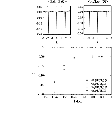
FIG. 14.: Above: Nonlinear cross-correlations $C^{n}_{12}(k,k^{\prime}=0)$ (left) and $C^{n}_{12}(k^{\prime}=0,k)$ (right) as function of $k$ for $E/E_{t}=0.999999$. Below: Semi-log plot the nonlinear correlations $C^{n}_{ij}(k=+k_{c},k^{\prime}=0)$ as function of $E/E_{t}$.

VII Correlations above threshold

Above the threshold for pattern formation the linearized equations (III) are no longer valid. As displayed in Fig. 4, above the threshold not only the homogeneous modes, but also all modes with wave numbers $k=\pm k_{c},\pm 2k_{c},\pm 3k_{c},\ldots$, will present a macroscopic photon number. Linearizing around the steady state pattern solution above the threshold under the assumption of small fluctuations, one obtains new linear equations for the far field fluctuation amplitudes, which take into account three-wave processes such as $[2\omega](k_{c})\leftrightarrow[\omega](k)+[\omega](k_{c}-k)$ or $[2\omega](k)\leftrightarrow[\omega](k_{c})+[\omega](k-k_{c})$. In analogy to the situation below the threshold a linear fluctuation analysis above the threshold predicts, in addition to the correlations already present below the threshold, the existence of additional correlations between the fluctuations $\delta I_{1}(k)$ and $\delta I_{1}(k_{c}-k)$, and between $\delta I_{2}(k)$ and $\delta I_{1}(k-k_{c})$. We will not report here the explicit results of this cumbersome linear analysis and restore directly to the numerical analysis of the full nonlinear Langevin equations.

FIG. 15.: The self-correlations a) $C^{n}_{11}(k,-k)$, b) $C^{n}_{22}(k,-k)$ and cross-correlations c) $C^{n}_{12}(k,k)$, d) $C^{n}_{12}(k,-k)$ as function of the transverse wave number for $E/E_{t}=1.05$.

To investigate the implications of the new field configuration above the threshold on the intensity correlations, we first consider the correlations $C^{n}_{ij}(k,k^{\prime})$. The same normalized correlations discussed in Fig. 7 below the threshold are plotted in Fig. 15 for a pump value above the threshold. We observe that the correlations at $k=\pm k_{c}$ decrease from their threshold value and are no longer perfect as they were at the threshold. A closer look actually reveals a dip in the correlations exactly at the pixels corresponding to $k=\pm k_{c}$. A tentative explanation for this is based on the fact that now the modes at the critical wave number have a finite average value, connected with macroscopic photon numbers in these modes, whereas the neighbouring pixels are significantly less populated, cf. the far field of Fig. 4. In comparison the normalized correlations $C^{n}_{ij}(k,k^{\prime})$ show a much smoother behaviour around $k_{c}$. Hence, the observed reductions in the correlations above threshold at $k=\pm k_{c}$ are connected with spontaneous population exchanges between these macroscopically populated modes.

In Fig. 8 the peaks at $k=\pm k_{c}$ of Fig. 15 are followed as function of the pump. The behavior is very similar to what is seen below the threshold. Close to the threshold the correlations are perfect, and as the pump is taken further away from $E_{t}$ the correlations become weaker. Below the threshold this was explained through an eigenvalue competition, while above the threshold the explanation is that the competitions between the states become stronger.

The $k=0$ cross-correlation is plotted in Fig. 9, and above the threshold there is a loss of anticorrelation or there is even a small positive correlation. This might be attributed to the macroscopic and independent occurrences of the processes of step 2) and 3) in Fig. 6.

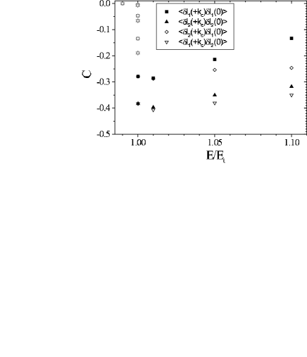
FIG. 16.: The correlations $C^{n}_{ij}(k=+k_{c},k^{\prime}=0)$ as function of the pump relative to the threshold. The gray symbols are the correlations below the threshold from Fig. 14.

FIG. 17.: Photon number variances for $E/E_{t}=1.05$ showing $C_{11}^{(-)}(k,-k)$ (diamonds) and $C_{11}^{(+)}(k,-k)$ (squares) from a numerical simulation.

We saw in Sec. VI B nonlinear correlations just below the threshold, and in Fig. 16 the peaks corresponding to these correlations are plotted in order to follow the progress above the threshold. The strongest anti-correlation is observed just above the threshold, $E/E_{t}=1.0001$ and as the pump is increased the correlations become weaker due to increasing competition of processes involving higher harmonics. Moreover, the connection between the self-correlations and cross-correlations seen below $E_{t}$ only remains very close to the threshold, so as the pump is increased $C^{n}_{11}(0,+k_{c})\neq C^{n}_{12}(0,+k_{c})$ and $C^{n}_{22}(+k_{c},0)\neq C^{n}_{12}(+k_{c},0)$. This is related to the loss of perfect correlations away from the threshold.

In Fig. 17 the photon number variances $C_{11}^{(\pm)}(k,-k)$ above the threshold are presented. Comparing these results with the corresponding ones below the threshold from Fig. 10 we observe that they are very similar. Generally, the correlation $C_{11}^{(-)}(k,-k)$ does not change much with the pump level, and this fact has also been observed in the OPO [36]. The sum correlation $C_{11}^{(+)}(k,-k)$, however, contains peaks that are very sensitive to the pump level, both below and above the threshold. The behavior discussed here for the FH is also valid for the SH and the cross-correlations.

VIII Conclusion and discussion

We have used the master equation approach to describe the spatiotemporal dynamics of the boson intra-cavity operators in second-harmonic generation, and we included in the model quantum noise as well as diffraction. Our study is based on the Q representation to describe the dynamics of the quantum fields in terms of a set of nonlinear stochastic Langevin equations for equivalent c-number fields. The choice of the Q representations gives some restraints on the parameter space, but we have checked that similar results are obtained using the approximated Wigner representation in other parameter regions.

A simple scheme describing the microscopic photon interaction that underlies the process of pattern formation has guided us in our analytical and numerical studies of the spatial correlations. Equal time correlations between intensity fluctuations were used to investigate the strength of the correlations between different modes. Also, possible nonclassical effects, such as twin beam correlations, were considered by calculating the photon number variances of the intensity sums and differences between spatial modes of the FH and SH fields.

We have found that at the threshold for pattern formation the Fourier modes with the critical wave number are perfectly correlated for the FH field, the SH field and also between the FH and the SH field. As the distance to the threshold is increased these correlations become weaker, which was shown analytically to be due to the competition of the eigenvalues of the linear system describing the system below the threshold. At large wave numbers, only the correlation between opposite points of the FH far field survives. This correlation is always found to be stronger than the others, which is consistent with the fact that the twin photon emission at the fundamental frequency is the primary source for correlations in the system. For far field modes around the critical wave number the self-correlations as well as the cross-correlations between FH and SH photons are linked to the pattern forming instability.

Very close to the threshold the linear analysis breaks down. The numerical simulations below the threshold showed the existence of nonlinear correlations which involve the $k=0$ mode and these are also seen above the threshold. The other correlations described above are also found above the threshold, but their strength decreases when moving away from the threshold. This can be understood from the fact that additional processes come into play, mainly consisting in population exchanges between the macroscopic fields at the critical wave number and its harmonics.

The intensity differences between opposite points of both the FH and SH far fields, as well as the cross-correlation between the two have been shown to exhibit nonclassical sub-shot noise behavior. These properties for the intensity difference turn out not to be sensitive to the process of pattern formation, since the corresponding correlations depend very weakly on the distance to the threshold and show no particular structure close to the critical wave number. The emerging pattern is connected with increased fluctuations in the modes with wave numbers around the critical wave number, leading to an excess noise in the corresponding individual intensities. Therefore, the sub-Poissonian statistics of the intensity differences reveal a partial noise cancellation. On the contrary, the sum of intensities clearly exhibit peaks around the critical wave number, originating from excess noise connected with the formation of a pattern.

In this work we considered equal time correlations calculated for the intra-cavity fields. This approach turned out to be very useful to understand the intra-cavity field dynamics. For the output fields we expect that the nonclassical correlations of the intra-cavity fields will remain below shot noise. The quantitative assessment of the amount of noise reduction or excess noise with respect to the shot noise level requires a specific additional calculation. For future work it would also be interesting to calculate the output fluctuation spectra at $0$ frequency for the difference and sum of intensities, which reflect the full amount of quantum correlations induced by the microscopic processes taking place inside the cavity, as for example considered for a vectorial Kerr model in [30].

IX Acknowledgments

We acknowledge financial support from the European Commission projects QSTRUCT (FMRX-CT96-0077), QUANTIM (IST-2000-26019) and PHASE and from the Spanish MCyT project BFM2000-1108. We thank Steve Barnett and Pere Colet for helpful discussions on this topic.

REFERENCES

- [1] M. C. Cross and P. C. Hohenberg, Rev. Mod. Phys. 65, 851 (1993).
- [2] Special issue on Transverse Effects in Nonlinear Optical Systems, edited by N. B. Abraham and W. J. Firth (J. Opt. Soc. Am. B, 951, 1990), Vol. 7.
- [3] Special issue on ”Nonlinear optical structures, patterns, chaos, edited by L. A. Lugiato (Chaos, Solitons and Fractals, 1249, 1994), Vol. 4.
- [4] F. T. Arecchi, S. Boccaletti, and P. Ramazza, Phys. Rep. 318, 1 (1999).
- [5] L. A. Lugiato and R. Lefever, Phys. Rev. Lett. 58, 2209 (1987).
- [6] C. Etrich, U. Peschel, and F. Lederer, Phys. Rev. E 56, 4803 (1997).
- [7] M. I. Kolobov, Rev. Mod. Phys. 71, 1539 (1999).
- [8] L. A. Lugiato, M. Brambilla, and A. Gatti, in Advances in atomic, molecular and optical physics, edited by B. Bederson and H. Walther (Academic, Boston, 1999), Vol. 40, p. 229.
- [9] L. A. Lugiato and P. Grangier, J. Opt. Soc. Am. B 14, 225 (1997).
- [10] L. Lugiato and G. Grynberg, Europhysics Letters 29, 675 (1995).
- [11] L. A. Lugiato and A. Gatti, Phys. Rev. Lett. 70, 3868 (1993).
- [12] G.-L. Oppo, M. Brambilla, and L. A. Lugiato, Phys. Rev. A 49, 2028 (1994).
- [13] A. Gatti, H. Wiedemann, L. A. Lugiato, I. Marzoli, G.-L. Oppo, and S. M. Barnett, Phys. Rev. A 56, 877 (1997).
- [14] P. Lodahl and M. Saffman, Opt. Lett. 27, 110 (2002).
- [15] C. W. Gardiner and P. Zoller, Quantum Noise, 2 ed. (Springer, Berlin, 2000).
- [16] M. Hillery, R. F. O’Connell, M. O. Scully, and E. P. Wigner, Phys. Rep. 106, 121 (1984).
- [17] W. S. Schleich, Quantum Optics in Phase Space (Wiley-VCH, Berlin, 1997).
- [18] P. Kinsler and P. D. Drummond, Phys. Rev. A 43, (1991).
- [19] P. D. Drummond and C. W. Gardiner, J. Phys. A: Math. Gen. 13, 2353 (1980).
- [20] H. P. Yuen and P. Tombesi, Opt. Comm. 59, 155 (1986).
- [21] A. Gilchrist, C. W. Gardiner, and P. D. Drummond, Phys. Rev. A 55, 3014 (1997).
- [22] R. Zambrini and S. M. Barnett, submitted, (2001).
- [23] R. Zambrini, S. M. Barnett, P. Colet, and M. San Miguel, unpublished, (2002).
- [24] C. M. Savage, Phys. Rev. A 37, 158 (1988).
- [25] In fact, in the present model both Ito and Stratonovich rules for interpreting the stochastic integration give identical results.
- [26] We note that Lodahl et al. [37, 38] showed that the pattern formation properties of the system considered here are modified by the presence of a competing parametric process, where the SH down-converts to non-degenerate parametric photons. For this stabilizes the system and can prevent pattern formation. In this study we neglect this competing parametric process.
- [27] The steady states and eigenvalues are calculated through a semi-analytical treatment using Mathematica. This also holds for the rest of the analytical results.
- [28] M. Bache, unpublished, (2001).
- [29] We use a Fourier split-step routine where the nonlinear terms are calculated in real space, and using a random number generator [39] to generate the Gaussian white noise terms. The number of spatial grid points was and the length of the system was adopted to fit in an integer multiple of the modulations in the near field, here chosen to 30. The pump field was taken as flat, i.e. independent of the position in the transverse plane. The time step was set to and checked to be stable. The correlations presented in this paper were all calculated after transients from the system was removed, and the averages were done over time and over several long trajectories, assuming that the system is ergodic. The data was sampled between and times with a time interval of 1 cavity lifetime, corresponding to sampling every integration steps.
- [30] R. Zambrini, M. Hoyuelos, A. Gatti, P. Colet, L. Lugiato, and M. S. Miguel, Phys. Rev. A 62, 063801 (2000).
- [31] L. Davidovich, Rev. Mod. Phys. 68, 127 (1996).
- [32] M. Hoyuelos, P. Colet, and M. San Miguel, Phys. Rev. E 58, 74 (1998).
- [33] R. Graham, Phys. Rev. Lett. 52, 117 (1984).
- [34] A. S. Lane, M. D. Reid, and D. F. Walls, Phys. Rev. A 38, 788 (1988).
- [35] M. Olsen, S. Granja, and R. Horowicz, Opt. Comm. 165, 293 (1999).
- [36] A. Heidmann, R. J. Horowicz, S. Reynaud, E. Giacobino, C. Fabre, and G. Camy, Phys. Rev. Lett. 59, 2555 (1987).
- [37] P. Lodahl, M. Bache, and M. Saffman, Opt. Lett. 25, 654 (2000).
- [38] P. Lodahl, M. Bache, and M. Saffman, Phys. Rev. A 63, 023815 (2001).
- [39] R. Toral and A. Chakrabarti, Compute Physics Communications 74, 327 (1993).