Dynamics of quantum adiabatic evolution algorithm for
Number Partitioning

Abstract

We have developed a general technique to study the dynamics of the quantum adiabatic evolution algorithm applied to random combinatorial optimization problems in the asymptotic limit of large problem size $n$. We use as an example the NP-complete Number Partitioning problem and map the algorithm dynamics to that of an auxilary quantum spin glass system with the slowly varying Hamiltonian. We use a Green function method to obtain the adiabatic eigenstates and the minimum excitation gap, $g_{\rm min}={\cal O}(n\,2^{-n/2})$, corresponding to the exponential complexity of the algorithm for Number Partitioning. The key element of the analysis is the conditional energy distribution computed for the set of all spin configurations generated from a given (ancestor) configuration by simulteneous fipping of a fixed number of spins. For the problem in question this distribution is shown to depend on the ancestor spin configuration only via a certain parameter related to the energy of the configuration. As the result, the algorithm dynamics can be described in terms of one-dimenssional quantum diffusion in the energy space. This effect provides a general limitation on the power of a quantum adiabatic computation in random optimization problems. Analytical results are in agreement with the numerical simulation of the algorithm.

I Introduction

Since the discovery by Shor Shor nearly a decade ago of a quantum algorithm for efficient integer factorization there has been a rapidly growing interest in the development of new quantum algorithms capable of solving computational problems that are practically intractable on classical computers. Perhaps the most notable example is that of a combinatorial optimization problem (COP). In the simplest case the task in COP is to minimize the cost function (“energy”) $E_{\bf z}$ defined on a set of $2^{n}$ binary strings ${\bf z}=\{z_{1},\ldots,z_{n}\}$ $z_{j}=0,1$, each containing $n$ bits. In quantum computation this cost function corresponds to a Hamiltonian $H_{P}$

$$H_{P}=\sum_{\bf z}E_{\bf z}|{\bf z}\rangle\langle{\bf z}|$$ (1)

$$|{\bf z}\rangle=|z_{1}\rangle_{1}\,\otimes|z_{2}\rangle_{2}\,\otimes\cdots\otimes|z_{n}\rangle_{n}.$$

where $z_{j}=0,1$ and the summation is over $2^{n}$ states $|{\bf z}\rangle$ forming the computational basis of a quantum computer with $n$ qubits. State $|z_{j}\rangle_{j}$ of the $j$-th qubit is an eigenstate of the Pauli matrix $\hat{\sigma}_{z}$ with eigenvalue $S_{j}=1-2z_{j}\,\,(S_{j}=\pm 1)$. It is clear from the above that the ground state of $H_{P}$ encodes the solution to the COP with cost function $E_{\bf z}$.

COPs have a direct analogy in physics, related to finding ground states of classical spin glass models. In the example above bits $z_{j}$ correspond to Ising spins $S_{j}$. The connection between the properties of frustrated disordered systems and the structure of the solution space of complex COPs has been noted first by Fu and Anderson Anderson . It has been recognized Parizi that many of the spin glass models are in almost one-to-one correspondence with a number of COPs from theoretical computer science that form the so-called NP-complete class Garey . This class contains hundreds of the most common computationally hard problems encountered in practice, such as constraint satisfaction, traveling salesmen, and integer programming. NP-complete problems are characterized in the worst cases by exponential scaling of the running time or memory requirements with the problem size $n$. A special property of the class is that any NP-complete problem can be converted into any other NP-complete problem in polynomial time on a classical computer; therefore, it is sufficient to find a deterministic algorithm that can be guaranteed to solve all instances of just one of the NP-complete problems within a polynomial time bound. It is widely believed, however, that such an algorithm does not exist on a classical computer; whether it exists on a quantum computer is one of the central open questions. Ultimately, one can expect that the behavior of new quantum algorithms for COPs and their complexity will be closely related to the properties of quantum spin glasses.

Recently, Farhi and co-workers suggested a new quantum algorithm for solving combinatorial optimization problems which is based on the properties of quantum adiabatic evolution Farhi . Running of the algorithm for several NP-complete problems has been simulated on a classical computer using a large number of randomly generated problem instances that are believed to be computationally hard for classical algorithms FarhiSc ; FarhiSat ; FarhiCli ; Hogg . Results of these numerical simulations for relatively small size of the problem instances ( $n\leq$ 20) suggest a quadratic scaling law of the run time of the quantum adiabatic algorithm with $n$. Furthermore, it was shown in Vazirani02 that the previous query complexity argument that led to the exponential lower bound for unstructured search Bennett cannot be used to rule out the polynomial time solution of NP-complete Satisfiability problem by the quantum adiabatic algorithm.

In Vazirani01 ; annealing ; Vazirani02 ; farhimeas ; BS special symmetric cases of COP were considered where symmetry of the problem allowed the authors to describe the true asymptotic behavior ($n\rightarrow\infty$) of the algorithm. In certain examples considered in Farhi ; annealing the quantum adiabatic algorithm finds the solution in time polynomial in $n$ while simulated annealing requires exponential time. This effect occurs due to the special connectivity properties of the optimization problems that lead to the relatively large matrix elements for the spin tunneling in transverse magnetic field between different valleys during the quantum adiabatic algorithm. In the examples considered in annealing the tunneling matrix element scales polynomially with $n$. On the other hand, in simulated annealing different valleys are connected via classical activation processes for spins with probabilities that scale exponentially with $n$. It was also shown for certain simplified examples farhimeas ; BS , that quantum adiabatic algorithm can be modified to completely suppress the tunneling barriers even if the corresponding classical cost function has local minima well separated in the space of spin configurations.

However, so far there are no study on the true asymptotic behavior of the algorithm for the general case of randomly generated hard instances of NP-complete problems. Also there are no analysis of the limitations of the quantum adiabatic computation arising from the intrinsic properties of disorder and frustration in this problems. Such analysis is of the central interest in this paper.

In Sec. II we introduce the random Number Partitioning problem and describes conditional cost distributions (neighborhood properties) in this problem. In Sec. III we describe the concept of quantum adiabatic computation applied to combinatorial optimization problems and introduce a Green function method for the analysis of the minimum gap. In Sec. IV we describe the effect of quantum diffusion in the algorithm dynamics, derive the scaling for the minimum gap and the complexity of the algorithm for the random Number Partitioning problem. We also obtain the scaling of the minimum gap numerically from the form of the cumulative density of the adiabatic eigenvalues at the avoided-crossing point. In Sec. V we discuss the results of the simulations of the time-dependent Schrödinger equation to simulate quantum adiabatic computation for Number Partitioning and obtain its complexity numerically.

II Number Partitioning Problem

Number Partitioning Problem (NPP) is one of the six basic NP-complete problems that are at the heart of the theory of NP-completeness Garey . It can be formulated as a combinatorial optimization problem:     Given a sequence of positive numbers $\{a_{1},\ldots,a_{n}\}$ find a partition, i.e. two disjoint subsets ${\cal A}$ and ${\cal A}^{\prime}$, such that the residue

$$E=\left|\sum_{a_{j}\in{\cal A}}a_{j}-\sum_{a_{j}\in{\cal A}^{\prime}}a_{j}\right|$$ (2)

is minimized. In NPP we search for the bit strings ${\bf z}=\{z_{1},\ldots,z_{n}\}$ (or corresponding Ising spin configurations ${\bf S}=\{S_{1},\ldots,S_{n}\}$) that minimize the energy or cost function $E_{\bf z}$

$$E_{\bf z}=\left|\Omega_{\bf S}\right|,\quad\Omega_{\bf S}=\sum_{j=1}^{n}a_{j}S_{j},\,\,S_{j}=1-2z_{j},$$ (3)

where $S_{j}=1$ ($z_{j}=0$) if $a_{j}\in{\cal A}$ and $S_{j}=-1$ ($z_{j}=1$) if $a_{j}\in{\cal A}^{\prime}$. The partition ${\bf S}$ with minimum residue can also be viewed as the ground state of the Ising spin glass, $-\Omega_{\bf S}^{2}$, corresponding to the Mattis-like antiferromagnetic coupling, $J_{ij}=-a_{i}\,a_{j}$.

NPP has many practical applications including multiprocessor scheduling ms , cryptography cr , and others. The best deterministic heuristical algorithm for NPP, the differencing method of Karmakar and Karp Karp , can find with high probability solutions whose energies are of the order $1/n^{\alpha\,\log\,n}$ for some $\alpha>0$. The interest in NPP also stems from the remarkable failure of a standard simulated annealing algorithm for the energy function (3) to find good solutions, as compared with the solutions found by deterministic heuristics johnson . The apparent reason for this failure is due to the existence of order $2^{n}$ local minima whose energies are of the order of $1/n$ Ferreira which undermines the usual strategy of exploring the space of the spin configurations ${\bf S}$ through single spin flips.

The computational complexity of random instances of NPP depends on the number of bits $b$ needed to encode the numbers $a_{j}$. In what follows we will analyze NPP with independent, identically distributed (i.i.d.) random b-bit numbers $a_{j}$. Numerical simulations show Gent ; Korf ; MertensCompleteAnytime that solution time grows exponentially with $n$ for $n\ll b$ then decreases steeply for $n\gtrsim b$ (phenomenon of “peaking”) and eventually grows polynomially for $n\gg b$. The transition from the “hard” to computationally “easy” phases at $n\approx b$ has features somewhat similar to phase transitions in physical systems Mertens98 . The detailed theory of the phase transition in NPP was given in Refs. Borgs1 ; Borgs2 . If one keeps the parameter $\xi=b/n$ fixed and lets $n\rightarrow\infty$ then instances of NPP corresponding to $\xi>$ 1 will have no perfect partitions with high probability. On the other hand for $\xi<$ 1 number of perfect partitions will grow exponentially with $n$. Transitions of this kind were observed in various NP-complete problems AI96 . In what follows we will focus on the computationally hard regime $\xi\gg 1$.

II.1 Distribution of signed partition residues

The values of individual energies are random and depend on the particular instance of NPP (i.e., the set of numbers $a_{j}$). However on a coarse-grained scale (i.e. after averaging over individual energy separations) the form of the typical energy distribution is described by some universal function for randomly generated problem instances. We introduce for a given set of randomly sampled numbers $a_{j}$ a coarse-grained distribution function of signed partition residues $\Omega_{\bf z}$ (3)

$$P(\Omega)=2^{-n}\frac{1}{\Delta\Omega}\int_{\Omega-\Delta\Omega/2}^{\Omega+\Delta\Omega/2}d\eta\sum_{{\bf z}\in\{0,1\}^{n}}\delta(\eta-\Omega_{\bf z}).$$ (4)

Here $\delta(x)$ is the Dirac delta-function; the sum is over $2^{n}$ bit-strings ${\bf z}$ and $2^{-n}$ is a normalization factor. In (4) we average over an interval $\Delta\Omega$ of the partition residues whose size is chosen self-consistently, $\Delta\Omega\gg 2^{-n}/P(\Omega)$. Using (3) we can rewrite (4) in the form

$$P(\Omega)=\frac{1}{2\pi}\int_{0}^{\infty}ds\,\zeta\left(\frac{\Delta\Omega\,s}{2}\right)\,I(s)\,\cos(\Omega s),$$ (5)

$$I(s)=\prod_{j=1}^{n}\cos(a_{j}\,s),\quad\zeta(x)=\sin(x)/x.$$

Here $\zeta(x)$ is a window function that imposes a cut-off in the integral (5) at $s\sim 2/\Delta\Omega$. For large $n$ this integral can be evaluated using the steepest descent method. In the following we shall assume that the $b$-bit numbers $a_{j}$ are distributed inside of the unit interval $[0,1]$ and are integer multiples of $2^{-b}$, the smallest number that can be represented with available number of bits $b$. We note that for large $n$ the function $I(s)$ has sharp maxima (minima) with width $\sim n^{-1/2}$ at the points $s_{k}=k\pi\,2^{b},\,k=0,1,\ldots;$ $|I(s_{k})|=1$. Only one saddle point at $s=0$ contributes to the integral in (5) due to coarse-graining of the distribution (4). Indeed, it will be seen below that the window size $2/\Delta\Omega$ can be chosen to obey the conditions ${\rm 1}\ll n^{{\rm 1/2}}/\Delta\Omega\ll{\rm 2}^{n}$. Therefore in the case of high-precision numbers, $b\gg n$, saddle-points $s_{k}$ with $k>0$ lie far outside the window and their contributions can be neglected (see also Appendix A). On the other hand the window function $\zeta(x)$ can be replaced by unity while computing the contribution from the saddle-point at $s=0$. Finally we obtain for $|\Omega|\ll n$ (cf. Mertens2000 )

$$P(\Omega)=\frac{1}{\sqrt{2\,\pi\,\sigma^{2}(0)\,n}}\exp\left(-\frac{\Omega^{2}}{2\sigma^{2}(0)\,n}\right)+{\cal O}(n^{-3/2})$$

$$\sigma^{2}(0)=\frac{1}{n}\sum_{j=1}^{n}a_{j}^{2}\qquad(E\ll n).$$ (6)

The coarse-grained distribution $P(\Omega)$ depends on the set of $a_{j}$’s through a single self-averaging quantity $\sigma(0)$ (cf. Mertens98 ).

One can also introduce the distribution $\tilde{P}(E)$ of cost values (energies) $E_{\bf z}=|\Omega_{\bf z}|$. Due to the obvious symmetry of the NPP, the cost function $E_{\bf z}$ in (3) does not change after flipping signs of all spins, $S_{j}\rightarrow-S_{j}$. Therefore

$$\tilde{P}(E)=1/2P(\pm E).$$ (7)

We emphasize that, according to Eq. (6) for a typical set of high-precision numbers $a_{j}$ the energy spectrum in NPP is quasi-continuous, and there are only two scales present in the distribution $\tilde{P}(E)$: one is a “microscopic” scale given by the characteristic separation of the individual partition energies, $E_{\rm min}$, and another is given by the mean partition energy $\langle E\rangle$ (or the distribution width $\langle E^{2}\rangle^{1/2}$)

$$E_{\rm min}\sim\sigma(0)\,n^{1/2}\,\,2^{-n},\qquad\langle E^{2}\rangle=\frac{\pi}{2}\langle E\rangle^{2}=n\sigma^{2}(0).$$ (8)

This justifies the choice for $\Delta\Omega$ above that corresponds to coarse-graining over many individual energy level separations.

We note that the distribution $P(\Omega)$ (6) is Gaussian for $E\ll n$ and can be understood in terms of a random walk with coordinate $\Omega$ using Eq. (3). The walk begins at the origin, $\Omega=0$, and makes a total of $n$ steps. At the $j$-th step $\Omega$ moves to the right or to the left by “distance” $2\,a_{j}$ if $S_{j}=1$ or $S_{j}=-1$, respectively. In the asymptotic limit of large $n$ the result (6) corresponds to equal probabilities of right and left moves and the distribution of step lengths coinciding with that of the set of numbers $\{2\,a_{j}\}$.

Finally, the energy distribution function $P(E)$ of the form (6),(7) was previously obtained by Mertens Mertens2000 using explicit averaging over the random instances of NPP. He also computed the partition function $Z(T)$ for a given instance of NPP at a small finite temperature $T$ using the steepest-descent method and summation over the saddle-points $s_{k}=k\pi\,2^{b}$ similar to our discussion above Mertens98 (in his analysis $k_{B}\,T$ played a role similar to our regularization factor $\Delta\Omega$ in (4),(5)).

We emphasize however, that the approach in Ref. Mertens98 based on $Z(T)$ is necessarily restricted to the analysis of the “static” properties of NPP at $E\sim 2^{-n}$, i.e., the phase transition in the number of perfect partitions Mertens98 when the control parameter $\xi=n/b$ crosses a critical value. On the other hand distribution $P(\Omega)$ (4) introduces at finite energies, as well as the conditional distribution introduced in the next section also allow us to directly study the intrinsic dynamical properties of the problem in question such as the dynamics of its quantum optimization algorithms.

II.2 Conditional distribution of signed partition residues

Consider the set of bit-strings ${\bf z^{\prime}}$ obtained from a given string ${\bf z}$ by flipping $r$ bits. The conditional distribution of the partition residues $\Omega_{\bf z^{\prime}}$ (3) in the $r$-neighborhood of ${\bf z}$ can be characterized by its moments:

$$\langle\Omega^{k}\rangle=\binom{n}{r}^{-1}\sum_{{\bf z^{\prime}}\in\{0,1\}^{n}}\left(\Omega_{\bf z^{\prime}}\right)^{k}\,\delta_{r,D({\bf z^{\prime}},{\bf z})},\qquad k=1,2,\ldots$$ (9)

Here $\delta_{m,l}$ is a Kronecker delta and function $D({\bf z},{\bf z^{\prime}})$ computes the number of bits that take different values in the bit-strings ${\bf z}$ and ${\bf z^{\prime}}$. It is the so-called Hamming distance between the two strings

$$D({\bf z},{\bf z^{\prime}})=\sum_{j=1}^{n}\left|z_{j}-z_{j}^{\prime}\right|.$$ (10)

The Hamming distance $r=D({\bf z},{\bf z^{\prime}})$ between the bit-strings is directly related to the overlap factor $q$ between the corresponding spin configurations often used in the theory of spin glasses Parizi ; Mertens2000 :

$$q=\frac{1}{n}\sum_{j=1}^{n}S_{j}S_{j}^{\prime}=1-\frac{2}{n}D({\bf z},{\bf z^{\prime}}).$$ (11)

(in what follows we shall use both quantities $r$ and $q$). For $k=1,2$ in (9) one obtains after straightforward calculation the first and second moments of the conditional distribution

$$\langle\Omega\rangle=q\,\Omega_{\bf z},$$ (12)

$$\langle\Omega^{2}\rangle-\langle\Omega\rangle^{2}=n\sigma^{2}(q)\,\left(1+\frac{1}{n-1}\right)\,\left(1-\frac{1}{n}\,\frac{\Omega_{\bf z}^{2}}{\langle E^{2}\rangle}\right),$$ (13)

$$\sigma(q)=\sigma(0)\,(1-q^{2})^{1/2},\qquad q\equiv 1-\frac{2r}{n},$$ (14)

where $\sigma(0)$ and $\langle E^{2}\rangle$ are given in (6) and (8), respectively.

The conditional distribution of $\Omega_{\bf z^{\prime}}$ can also be defined in a way similar to (4)

$$P_{r,{\bf z}}(\Omega^{\prime})=\binom{n}{r}^{-1}\,\frac{1}{\Delta\Omega^{\prime}}\int_{\Omega^{\prime}-\Delta\Omega^{\prime}/2}^{\Omega^{\prime}+\Delta\Omega^{\prime}/2}d\eta\sum_{\bf z^{\prime}\in\{0,1\}^{n}}\delta(\eta-\Omega_{\bf z^{\prime}})\,\delta_{r,D({\bf z^{\prime}},{\bf z})}$$ (15)

where averaging is over the small interval $\Delta\Omega^{\prime}$ that, however, includes many individual values of $\Omega_{z^{\prime}}$ for a given $r$. It is clear from (12),(13) that the first two moments of $P_{r,{\bf z}}(\Omega^{\prime})$ depend on ${\bf z}$ only via the value of $\Omega_{\bf z}$. This does not hold true, however, for the higher-order moments that depend on other functions of ${\bf z}$ as well. For example, $\langle\Omega^{3}\rangle$ involves the quantity $\sum_{j=1}^{n}a_{j}^{3}(1-2z_{j})$, etc.

Our main observation is that in the asymptotic limit of large $n$ the conditional distribution $P_{r,{\bf z}}(\Omega^{\prime})$ is well-described by the first two moments (12),(13). Then, according to the discussion above, its dependence on ${\bf z}$ is only via $\Omega_{\bf z}$. The detailed study of the higher moments (9) will be done elsewhere. Here we use the following intuitive approach relevant for analysis of the computational complexity of the quantum adiabatic algorithm for the NPP. We average $P_{r,{\bf z}}(\Omega^{\prime})$ over the strings ${\bf z}$ with residues $\Omega_{\bf z}$ inside a small interval $\Delta\Omega$ (containing, however, many levels $\Omega_{\bf z}$). After such averaging the result, $P_{r}(\Omega^{\prime}|\Omega)$, can be written in the form

$$P_{r}(\Omega^{\prime}|\Omega)=\frac{P_{r}(\Omega^{\prime},\Omega)}{P(\Omega)},$$ (16)

$$P_{r}(\Omega^{\prime},\Omega)=2^{-n}\,\frac{1}{\Delta\Omega}\int_{\Omega-\Delta\Omega/2}^{\Omega+\Delta\Omega/2}d\eta\,\sum_{{\bf z}\in\{0,1\}^{n}}\,\delta(\eta-\Omega_{\bf z})\,P_{r,{\bf z}}(\Omega^{\prime}),$$ (17)

where $P(\Omega)$ is given in (6). We note that Eq. (16) formally coincides with the Bayesian rule expressing the conditional distribution function $P_{r}(\Omega^{\prime}|\Omega)$ through the 2-point (joint) distribution function $P_{r}(\Omega^{\prime},\Omega)$ and the single-point distribution $P(\Omega)$ (6).

The explicit form of $P_{r}(\Omega|\Omega)$ is derived in Appendix B in a manner similar to the derivation of $P(E)$ in Sec. II.1. The results are presented in Eqs. (72) and (73). They show that $P_{r}(\Omega^{\prime},\Omega)$ in the limit $n\gg 1$ is indeed well described by its first two moments that corresponds precisely to the expressions given in Eqs. (12),(13) above. From this we conclude that

$$P_{r,{\bf z}}(\Omega^{\prime})=P_{r}(\Omega^{\prime}|\Omega_{\bf z}).$$ (18)

In the case $r=1$ there are $n$ strings ${\bf z^{\prime}}$ at a Hamming distance 1 from the string ${\bf z}$. Partition energies corresponding to these strings equal $|\Omega_{\bf S}-2a_{j}S_{j}|,\,1\leq j\leq n$ (cf. (3)). After the coarse-graining over the energy scale ${\cal O}(1/n)$ in the range, $|\Omega|,|\Omega^{\prime}|\ll n$, the conditional distribution $P_{r,{\bf z}}$ is a step function in the interval $\Omega_{\bf z}-\Omega^{\prime}\in\left[-2,2\right]$. For $r=n-1$ one has the same form of the distribution but for $\Omega_{\bf z}+\Omega^{\prime}$. Both results correspond to nearly equal distribution of spins between between $\pm 1$ values. Then in the range of energies $|\Omega^{\prime}|,|\Omega_{\bf z}|\lesssim 1$ one has:

$$P_{r,{\bf z}}(\Omega^{\prime})\approx\bar{P}_{r}=1/2+{\cal O}\left(\frac{1}{n}\right),\quad r=1,n-1\qquad(n\gg 1)$$ (19)

For $r,n-r\gg 1$ distribution $P_{r,{\bf z}}(\Omega^{\prime})$ has a Gaussian form with a broad maximum at $\Omega^{\prime}=q\Omega_{\bf z}$ (cf. Eqs. (12),(13),(72)) . Near the maximum we have:

$$P_{r,{\bf z}}(\Omega^{\prime})\approx\bar{P}_{r}=\frac{1}{\sqrt{2\pi n\sigma^{2}(q)}},\qquad|\Omega^{\prime}|,|\Omega_{\bf z}|\ll n^{1/2}\sigma(q).$$ (20)

We studied the conditional distribution in NPP numerically as well (see Fig.1 and Sec.B). The results are in good agreement with theory even for modest values of $n\leq 30$.

Figure 1: Plots of the (scaled) conditional distribution (15) $s=\sigma(0)(2\pi n)^{1/2}\,(\Delta\Omega)^{-1}\int_{0}^{\Delta\Omega}d\eta\,P_{r,{\bf z}}(\eta)$ vs $r$ are shown with points. We use coarse-graining window $\Delta\Omega$=0.3. Different plots correspond to 29 randomly selected bit-strings ${\bf z}$ with energies $|\Omega_{\bf z}|\in[0,0.3]$ for one randomly generated instance of NPP with $n=30$ and $b=35$. For $r,n-r\gg 1$ the values of $s$ corresponding to different strings are visually indistinguishable from each other. Dashed line is a plot of $\sigma(0)/\sigma(q)$ vs $\,\,r$ given in (13) ($q=1-2r/n$).    Insert: plots of the integrated quantity given in (74), $Q=\frac{1}{2}\int_{0}^{\Omega}d\eta\,P_{r,{\bf z}}(\eta)$ vs $x=\Omega/(\sigma(q)\sqrt{2n})$, for different values of $r=2,\ldots,n/2$ and randomly selected bit-string ${\bf z}$ with energy $|\Omega_{\bf z}|$ close to 0. All plots correspond to the same instance of NPP as the main figure. Plots for different values of $r$ are visually indistinguishable from each other and from the theoretical curve given in (75).

The characteristic spacing between the values of the partition residues in the subset of strings ${\bf z^{\prime}}$ with $D({\bf z^{\prime}},{\bf z})=r$ is $1/(\bar{P}_{r}\,\binom{n}{r})$ for not too large $E_{\bf z},E_{\bf z^{\prime}}$ (see above). This spacing decreases exponentially with the magnitude of the string overlap factor, $|q|=|(n-2r)/n|$. The hierarchy of the subsets corresponding to different values of $|q|$ form a specific structure of NPP. We note that the distribution of partition residues within the hierarchy is nearly independent of the ancestor string ${\bf z}$ in a broad range of energies $E^{\prime}\lesssim n^{1/2}$ where $P_{r,{\bf z}}(E^{\prime})\approx\bar{P}_{r}$. One can see that the magnitude of the overlap factor $q$ between two strings with energies within a given interval $[0,E]$ is limited by some typical value $\bar{q}$ satisfying the following equation:

$$E\binom{n}{r}\bar{P}_{r}=1,\qquad|\bar{q}|=1-2\frac{r}{n}.$$ (21)

The smaller $E$ is, the smaller $|\bar{q}|$ is: strings that are close in energy are far away in the configuration space. This property gives rise to an exponentially large number of local minima for small values of $E_{\bf z}$ that are far apart in the configuration space. For example, strings with $E_{\bf z}\sim E_{\rm min}$ typically correspond to $|q|={\cal O}(1/n)$, they can be obtained from each other only by simultaneously flipping clusters with $\sim n/2$ spins.

Eq. (21) describes the dynamics of a local search heuristic (e.g., simulated annealing). It shows that the average cost value $E$ during the search decreases no faster than ${\cal O}(1/M)$ where $M={\cal O}\left(\binom{n}{r}\right)$ is the number of generated configurations. This result coincides with that obtained in Mertens2000 using a different approach. It says that any classical local search heuristic for NPP cannot be faster than random search. Indeed, during local search the information about the “current” string ${\bf z}$ with $E_{\bf z}\lesssim 1$ is being lost, on average, after one spin flip (cf. Eqs. (19),(20)). We show below that precisely this property of NPP also leads to the complexity of the quantum adiabatic algorithm corresponding to that of a quantum random search.

We note that one can trivially break the symmetry of NPP mentioned above by introducing an extra number $a_{0}$ and placing it, say, in the subset ${\cal A}$. In this case different partition energies will still be encoded by spin configurations ${\bf S}=\{S_{1},\ldots,S_{n}\}$ (or corresponding bit-strings ${\bf z}$) with $\Omega_{\bf S}=a_{0}+\sum_{j=1}^{n}S_{j}\,a_{j}$ and $E_{\bf z}=|\Omega_{\bf S}|$ (cf. 3). We shall adopt this approach in the analysis of the performance of the quantum adiabatic algorithm for NPP given below.

III Quantum Adiabatic Evolution Algorithm

In the quantum adiabatic algorithm Farhi one specifies the time-dependent Hamiltonian $H(t)=\tilde{H}(t/T)$

$$\tilde{H}(\tau)=(1-\tau)\,V+\tau\,H_{P},$$ (22)

where $\tau=t/T$ is dimensionless “time”. This Hamiltonian guides the quantum evolution of the state vector $|\psi(t)\rangle$ according to the Schrödinger equation $i\,{\partial|\psi(t)\rangle\partial t}=H(t)|\psi(t)\rangle$ from $t=0$ to $t=T$, the run time of the algorithm (we let $\hbar=1$). $H_{P}$ is the “problem” Hamiltonian given in (1). $V$ is a “driver” Hamiltonian, that is designed to cause transitions between the eigenstates of $H_{P}$. In this algorithm one prepares the initial state of the system $\psi(0)$ to be the ground state of $\tilde{H}(0)=V$. In the simplest case

$$V=-\sum_{j=1}^{n}\sigma_{x}^{j},\quad|\psi(0)\rangle=2^{-n/2}\sum_{\bf z}|{\bf z}\rangle,$$ (23)

where $\sigma_{x}^{j}$ is a Pauli matrix for $j$-th qubit. Consider instantaneous eigenstates $|\phi_{\eta}(\tau)\rangle$ of $\tilde{H}(\tau)$ with energies $\lambda_{\eta}(\tau)$ arranged in nondecreasing order at any value of $\tau\in(0,1)$

$$\tilde{H}|\phi_{\eta}\rangle=\lambda_{\eta}|\phi_{\eta}\rangle,\quad\eta=0,1,\ldots,2^{n}-1.$$ (24)

Provided the value of $T$ is large enough and there is a finite gap for all $t\in(0,T)$ between the ground and excited state energies, $g(\tau)=\lambda_{1}(\tau)-\lambda_{0}(\tau)>0$, quantum evolution is adiabatic and the state of the system $|\psi(t)\rangle$ stays close to an instantaneous ground state, $|\phi_{0}(t/T)\rangle$ (up to a phase factor). Because $H(T)=H_{P}$ the final state $|\psi(T)\rangle$ is close to the ground state $|\phi_{0}(\tau=1)\rangle$ of the problem Hamiltonian. Therefore a measurement performed on the quantum computer at $t=T\,(\tau=1)$ will find one of the solutions of COP with large probability.

There is a broad class of COPs from theoretical Computer Science where the number of distinct values of a cost function scales polynomially in the size of an input $n$. An example is the Satisfiability problem in which the cost $E_{\bf z}$ of a given string ${\bf z}$ equals the number of constrains violated by the string. For those problems, the spectrum of $H(\tau)$, at the beginning ($\tau\approx 0$) and at the end ($\tau\approx 1$) of the algorithm, consists of a polynomial number of well-separated energy levels. Quantum transitions away from the adiabatic ground state occur most likely near the avoided-crossing points $\tau\approx\tau^{*}$ where the energy gap $g(\tau)$ reaches its minima Hogg . Near the avoided-crossing points, the spectrum of $H(\tau)$ is quasi-continuous, with the separation between individuals eigenvalues scaled down with $n$. The probability of a quantum transition, $1-|\langle\psi(t)|\phi_{0}(t/T)\rangle|^{2}_{t=T}$, is small provided that

$$T\gg\frac{|\langle\phi_{1}|\tilde{H}_{\tau}|\phi_{0}\rangle|_{\tau=\tau^{*}}}{g_{\rm min}^{2}},\quad g_{\rm min}=\min_{0\leq\tau\leq 1}\left[\lambda_{1}(\tau)-\lambda_{0}(\tau)\right],$$ (25)

($\tilde{H}_{\tau}\equiv d\tilde{H}/d\tau$). The fraction in (25) gives an estimate for the required runtime of the algorithm and the task is to find its asymptotic behavior in the limit of large $n\gg 1$. The numerator in (25) is less than the largest eigenvalue of $\tilde{H}_{\tau}=H_{P}-V$, typically polynomial in $n$ Farhi . However, $g_{\rm min}$ can scale down exponentially with $n$ and in such cases the runtime of the quantum adiabatic algorithm will grow exponentially with the size of COP.

III.1 Implementation of QAA for NPP

As suggested in Farhi the quantum adiabatic algorithm can be recast within the conventional quantum computing paradigm using the technique introduced by Lloyd Lloyd . Continuous-time quantum evolution can be approximated by a time-ordered product of unitary operators, $e^{-i\,(1-\tau_{k})V\delta}\,e^{-i\tau_{k}H_{P}\delta}$, corresponding to small time intervals $(t_{k},t_{k}+\delta)$. Operator $e^{-i\,(1-\tau_{k})V\delta}$ typically corresponds to a sequence of 1- or 2-qubit gates (cf. (23)). Operator $e^{-i\tau_{k}H_{P}\delta}$ is diagonal in the computational basis $|{\bf z}\rangle$ and corresponds to phase rotations by angles $E_{\bf z}\delta$. Since in the case $n\ll b$, the average separation between the neighboring values of $E_{\bf z}$ is $1/P(E)={\cal O}(2^{-n})$, the quantum device would need to support a very high precision in its physical parameters (like external fields, etc.) to control small ${\cal O}(2^{-n})$ differences in phases. Since this precision scales with $n$ exponentially it would strongly restrict the size of an instance of NPP that could be solved on such a quantum computer. This technical restriction is generic for COPs that involve a quasi-continuous spectrum of cost-function values. Among the other examples are many Ising spin glass models in physics (e.g., the Sherrington-Kirkpatrick model Parizi ). To avoid this restriction we introduce a new oracle-type cost function ${\cal E}_{\bf z}$ that returns a set of values

$${\cal E}_{\bf z}=c(\Omega_{\bf z}),\qquad c(x)\longrightarrow\{\varepsilon_{0},\varepsilon_{1},\ldots,\varepsilon_{M}\}\qquad(\varepsilon_{k+1}>\varepsilon_{k}),$$ (26)

that can be stored using a relatively small number of bits ${\cal O}(\log n)$. For example, we can divide an interval of partition energies $(0,B)$, $B=\sum_{j=0}^{j=n}a_{j}$ into bins whose sizes grow exponentially with the energy. Then the new cost will take one value per bin

$$c(x)=\varepsilon_{k}\equiv-M+k\quad\qquad\,{\rm for}\,\,\omega_{k}\leq|x|<\omega_{k+1},$$

$$\omega_{k}=(2^{k}-1)\,\Delta,\quad k=0,\ldots,\,M.$$ (27)

The last bin is $\omega_{M}\leq|\Omega_{\bf z}|\leq B$ where we have ${\cal E}_{\bf z}=\varepsilon_{M}=0$. The value of the cutoff $\omega_{M}\leq B$ is discussed below. In this example the Hilbert space of $2^{n}$ states $|{\bf z}\rangle$ is divided into $M+1$ subspaces ${\cal L}_{k}$, each determined by Eq. (27) for a given $k$

$$H_{P}=\sum_{k=0}^{M}\varepsilon_{k}\sum_{{\bf z}\in{\cal L}_{k}}|{\bf z}\rangle\langle{\bf z}|.$$ (28)

Note that subspace ${\cal L}_{0}$ contains the solution(s) to NPP. Dimension $d_{0}$ of ${\cal L}_{0}$ is controlled by the value of $\Delta$ in (27) which is another control parameter of the algorithm. We set $\Delta=2^{-n}\,K/P(0)$ where the integer $K\approx d_{0}\gg 1$ is independent of $n$ and determines how many times on average one needs to repeat the quantum algorithm in order to obtain the solution to NPP with probability close to 1.

Operator $H_{P}$ projects any state $|\psi\rangle$ onto the states with partition residues in the range $0\leq|\Omega_{\bf z}|<\omega_{M}$. If we choose

$$1\lesssim\omega_{M}\ll\langle E\rangle,$$ (29)

then the distribution function (6) is nearly uniform for $|\Omega_{\bf z}|\leq\omega_{M}$. Therefore the dimensions of the subspaces ${\cal L}_{k}$ grow exponentially with $k$: $d_{k}=d_{0}\,2^{k}$ for $k<M$. This simplification would not affect the complexity of a quantum algorithm that spends most of its time in “annealing” the system to much smaller partition residues, $\omega_{M}\gg|\Omega_{\bf z}|\sim E_{\rm min}={\cal O}(n^{1/2}\,2^{-n})$.

We note that the new discrete-valued cost function defined in (27) is non-local. Unlike problems such as Satisfiability, it cannot be represented by a sum of terms each involving a small number of bits. To implement a unitary operator $e^{-i\tau_{k}H_{P}\delta}$ with $H_{P}$ given in (28) one needs to implement the following classical function on a quantum computer

$${\cal E}_{\bf z}=\Theta(\omega_{M}-|\Omega_{\bf z}|)\,\left[\log_{2}\left(\frac{\Delta+|\Omega_{\bf z}|}{\Delta+\omega_{M}}\right)\right],\qquad\Omega_{\bf z}=\sum_{j=1}^{n}a_{j}(1-2z_{j}).$$ (30)

Here $[x]$ denotes the integer part of a number $x$; $\Theta(x)$ is the theta-function ($\Theta(x)=1$ for $x\geq 0$ and $\Theta(x)=0$ for $x<0$). The implementation of (30) with quantum circuits involves, among other things, the addition of $n$ numbers together with their signs to compute $\Omega_{\bf z}$, and taking the discrete logarithm of a $b$-bit number with respect to base $2$. These operations can be performed using a number of quantum gates that is only polynomial in $n$ and $b$ (cf. Shor for the implementation of the discrete logarithm).

Since the implementation of a cost function (26),(30) does not add an exponential overhead to the complexity of QAA the feasibility of this algorithm for NPP depends on the scaling of the minimum gap $g_{\min}$ with $n$.

III.2 Stationary Schrödinger equation for adiabatic eigenstates

We now solve the stationary Schrödinger equation (24) and obtain the minimum gap $g_{\rm min}$ (25) in the asymptotic limit $n\rightarrow\infty$. To proceed we need to introduce a new basis of states $|{\bf x}\rangle=|x_{1}\rangle_{1}\,\otimes|x_{2}\rangle_{2}\,\otimes\cdots\otimes|x_{n}\rangle_{n}$ where state $|x_{j}\rangle_{j}$ is an eigenstate of the Pauli matrix $\hat{\sigma}_{x}$ for the $j$-th qubit with eigenvalue $1-2x_{j}=\pm 1$. Driver Hamiltonian $V$ can be written in the following form:

$$V=\sum_{m=0}^{n}\,V_{m}\,{\cal I}^{m},\,\,\,\,{\cal I}^{m}=\sum_{x_{1}+\cdots+x_{n}=m}|{\bf x}\rangle\langle{\bf x}|.$$ (31)

For a particular case given in Eq. (23) we have $V_{m}=2m-n$. Matrix elements of ${\cal I}^{m}$ in a basis of states $|{\bf z}\rangle$ depend only on the Hamming distance $D({\bf z},{\bf z^{\prime}})$ between the strings ${\bf z}$ and ${\bf z^{\prime}}$

$$\langle{\bf z}|{\cal I}^{m}|{\bf z^{\prime}}\rangle=I^{m}_{D({\bf z},{\bf z^{\prime}})},$$ (32)

$$I^{m}_{r}=2^{-n}\sum_{q=0}^{n-r}\sum_{p=0}^{r}\binom{n-r}{q}\binom{r}{p}(-1)^{p}\,\Delta_{m,\,q+p}.$$ (33)

We now rewrite Eq. (24) in the form

$$|\phi\rangle=\frac{\tau}{\lambda-\alpha V}\,H_{P}\,|\phi\rangle,\quad\alpha\equiv\alpha(\tau)=1-\tau,$$ (34)

(we drop the subscript $\eta$ indicating the number of a quantum state and also the argument $\tau$ in $\phi$ and $\lambda$). From (27)-(34) we obtain the equation for the amplitudes $\phi_{\bf z}=\langle{\bf z}|\phi\rangle$ in terms of the coefficients $I^{m}_{r}$

$$\left[1-\tau G_{0}\,c(\Omega_{\bf z})\right]\,\phi_{\bf z}=\frac{\tau\Phi\,2^{-n}}{\lambda-\alpha V_{0}}+\tau\sum_{{\bf z^{\prime}}\neq{\bf z}}G_{D({\bf z},{\bf z^{\prime}})}\,\phi_{\bf z^{\prime}}\,c(\Omega_{\bf z}),$$ (35)

$$\Phi=\sum_{\bf z^{\prime}}c(\Omega_{\bf z^{\prime}})\,\phi_{\bf z^{\prime}},$$

$$G_{r}\equiv G_{r}(\lambda)=\sum_{m=1}^{n}\frac{I^{m}_{r}}{\lambda-\alpha V_{m}},\quad 0\leq r\leq n.$$

Here we separated out a “symmetric” term $\propto 2^{-n}\Phi$ corresponding to the coupling between the states $|{\bf z}\rangle$ via the projection operator ${\cal I}^{0}$ (31).

IV Minimum gap analysis

IV.1 Coarse-graining of the transition matrix

We now make a key observation that $\phi_{\bf z}$ in (35) can be determined based on the properties of the conditional distribution $P_{r,{\bf z}}(E)$ (15) and the form of the Green function $G_{r}(\lambda)$. We sum the Green function $G_{D({\bf z},{\bf z^{\prime}})}$ over all possible transitions from a given state ${\bf z^{\prime}}$ to states ${\bf z^{\prime}}\neq{\bf z}$ with energy $\varepsilon_{k}$. For not too large partition residues of the initial and final states we obtain

$$\sum_{{\bf z}\in{\cal L}_{k},\,{\bf z}\neq{\bf z^{\prime}}}G_{D({\bf z},{\bf z^{\prime}})}(\lambda)\approx F_{k}(\lambda)+f_{{\bf z^{\prime}},k}(\lambda)$$ (36)

$$F_{k}(\lambda)=\frac{\mu\,s(\lambda)}{2^{M-k}},\,\,\,s(\lambda)=\int_{0}^{n}dr\,\frac{\sigma(0)}{\sigma\left(1-2r/n\right)}\binom{n}{r}G_{r}(\lambda)$$ (37)

$$|\Omega_{\bf z^{\prime}}|,\,|\Omega_{\bf z}|\ll\langle E\rangle,\qquad\mu=\frac{2\omega_{M}}{\pi\langle E\rangle}.$$ (38)

Function $\sigma(q)$ above is defined in (14) and $f_{{\bf z^{\prime}},k}(\lambda)$ is a small correction described below. In function $s(\lambda)$ we replaced summation over the integer values of $r$ by an integral. It can be evaluated using the explicit form of $G_{r}(\lambda)$ that decays rapidly with $r$. In what follows we will be interested in the region $|\lambda-\alpha V_{0}|\ll 1$ where

$$-2\alpha\,G_{r}(\lambda)=\binom{n}{r}^{-1}\sum_{m=1}^{n-r}\frac{2^{-n}\binom{n}{m+r}}{m}-2^{-n}\left(\ln r+\gamma\right).$$ (39)

($\gamma$ is Euler’s constant) and $s(\lambda)\approx-\ln 2/(2\alpha)$. We note that

$$-2\alpha\,G_{r}(\lambda)\approx-\left[(n/2-r)\binom{n}{r}\right]^{-1},\quad n/2-r\gg 1.$$ (40)

Therefore the integrand in $s(\lambda)$ is a smooth function of $r$ for $r\lesssim n/2$ and quickly decays to zero for $r\gtrsim n/2$. The contribution to the integral in $s(\lambda)$ from the range of $r\ll n$ is small (${\cal O}((r/n)^{1/2}$).

We note that term $F_{k}$ in (36) provides an “entropic” contribution to the sum in (36). It comes from the large number of states ${\bf z}\in{\cal L}_{k}$ corresponding to large Hamming distances $r$ from the state ${\bf z^{\prime}}$, $1\ll r\lesssim n/2$. Each state contributes a small weight, $G_{r}\propto\binom{n}{r}^{-1}$, and number of states for a given $r$ is large, $(\omega_{k+1}-\omega_{k})\,\binom{n}{r}\,\bar{P}_{r}\gg 1$. Here $(\omega_{k+1}-\omega_{k})$ is an energy bin for the subspace ${\cal L}_{k}$ and $\bar{P}_{r}$ is the conditional density of states described in Sec. II. The size of the bin scales down exponentially with $k$ (cf. (27)) and so does the entropic term $F_{k}$. Below a certain cross-over value of $k$ one has $|F_{k}|\ll|f_{{\bf z^{\prime}},k}(\lambda)|$. In this case the dominant contribution to the sum (36) comes from the states ${\bf z}$ with small $r=D({\bf z},{\bf z^{\prime}})\sim 1$. In particular for $k=0$ one can obtain

$$f_{{\bf z^{\prime}},0}(\lambda)\approx G_{1}(\lambda)\,\sum_{{\bf w}\in{\cal L}_{0}}\delta_{1,D({\bf z^{\prime}},{\bf w})}+{\cal O}(n^{-3}),$$ (41)

where the higher-order terms correspond to $D({\bf z^{\prime}},{\bf w})\geq$ 2. According to (39), $|G_{1}(\lambda)|\sim n^{-2}$ and therefore $|f_{{\bf z},0}|$ is exponentially larger than the entropic term, $|F_{0}|\sim\omega_{0}\sim d_{0}\,2^{-n}$. We note that, unlike the entropic term, $f_{{\bf z^{\prime}},0}$ strongly depends on ${\bf z^{\prime}}$ due to the discreteness of the partition energy spectrum ($\omega_{0}\,n\ll 1$). E.g., depending on a state ${\bf z^{\prime}}$, in this case there could be either one or none of the states ${\bf w}\in{\cal L}_{0}$ in the sum (41) satisfying $D({\bf z^{\prime}},{\bf w})=1$.

IV.2 Extended and localized eigenstates

Based on the discussion above we look for solution of Eq. (35) in the following form:

$$\phi_{\bf z}=v(\Omega_{\bf z})+u_{\bf z},\qquad{\bf z}\notin{\cal L}_{0},$$ (42)

where we have explicitly separated out a part of the wavefunction $v(\Omega_{\bf z})$ that depends on ${\bf z}$ only via the corresponding value of the partition residue. It satisfies the following equations:

$$\left[1-\tau\,G_{0}(\lambda)\,c(\Omega)\right]\,v(\Omega)=\frac{\tau\Phi\,2^{-n}}{\lambda-\alpha V_{0}}+\tau\int_{\infty}^{\infty}d\Omega^{\prime}\,v(\Omega^{\prime})\,c(\Omega^{\prime})\,\chi(\Omega^{\prime},\Omega,\lambda),$$ (43)

$$\chi(\Omega^{\prime},\Omega,\lambda)=\sum_{r=1}^{n}\binom{n}{r}\,G_{r}(\lambda)\,P_{r}(\Omega^{\prime}|\Omega).$$ (44)

where $\Phi$ is given in (35) and function $c(x)$ takes a set of discrete values (26). Using (35),(42) and (43) we obtain equations for $u_{\bf z}$

$$\left[1-\tau\,G_{0}(\lambda)\,\varepsilon_{k}\right]\,u_{\bf z}=\tau\,\sum_{k^{\prime}=1}^{M}\varepsilon_{k^{\prime}}\sum_{{\bf z^{\prime}}\in{\cal L}_{k}}G_{D({\bf z},{\bf z^{\prime}})}(\lambda)\,u_{\bf z^{\prime}}+\tau\varepsilon_{0}\sum_{{\bf w}\in{\cal L}_{0}}G_{D({\bf z},{\bf w})}(\lambda)\phi_{\bf w},\qquad{\bf z}\in{\cal L}_{k}.$$ (45)

Decomposition (42) is only applied to amplitudes $\phi_{\bf z}$ with ${\bf z}\notin{\cal L}_{0}$. The system of equations for the components $v(\Omega)$ and $u_{\bf z}$ is closed by adding Eq. (35) for the amplitudes $\phi_{\bf w}$ with ${\bf w}\in{\cal L}_{0}$ (ground states of the final Hamiltonian $H_{P}$) and taking (42) into account. We note that Eq.(43) for $v(\Omega)$ is coupled to the rest of the equations only via the symmetric term $\Phi$

$$\Phi=\overline{\Phi}+\widetilde{\Phi}+\Phi_{0}$$ (46)

$$\overline{\Phi}=2^{n}\,\int_{-\infty}^{\infty}dx\,P(x)\,v(x)\,c(x),$$ (47)

$$\widetilde{\Phi}=\sum_{k=1}^{M}\varepsilon_{k}\sum_{{\bf z}\in{\cal L}_{k}}u_{\bf z},\quad\Phi_{0}=\varepsilon_{0}\sum_{{\bf w}\in{\cal L}_{0}}\phi_{\bf w},$$

where distribution $P(\Omega)$ is given in (6).

IV.2.1 Minimum gap estimate for $\omega_{M}\ll\langle E\rangle$

We will analyze the above system of equations (42)-(47) assuming that the cutoff frequency $\omega_{M}$ satisfies Eq.(29). This condition corresponds to the linear region in the plot of the cumulative density of states given in insert to the Fig. II.1. According to Eqs. (6),(19), in this range the distribution functions $P(\Omega)\approx\bar{P}_{n/2}$ and $P_{r}(\Omega^{\prime}|\Omega)\approx\bar{P}_{r}$ take nearly constant values and spectral function $\chi(\Omega^{\prime},\Omega,\lambda)$ equals

$$\chi(\Omega^{\prime},\Omega,\lambda)\approx\frac{s(\lambda)}{\sqrt{2\pi\,n\,\sigma^{2}(0)}}.$$ (48)

where $s(\lambda)$ is given in (37). In this approximation, we can compute $\widetilde{\Phi}$ using equations for $u_{\bf z}$ in (45) and also the relations in (36), (37)

$$\widetilde{\Phi}=-\kappa\left(\tau\mu s(\lambda)\right)\Phi_{0},\qquad\kappa(x)=\frac{x}{1+x}.$$ (49)

In the initial stage of the algorithm the amplitudes $\phi_{\bf w}$ of the “solution” states are small $|\Phi_{0}|={\cal O}(2^{-n/2})$. According to (49), we also have $|\widetilde{\Phi}|={\cal O}(2^{-n/2})$. Neglecting these terms and setting $\Phi\approx\overline{\Phi}$, Eq. (43) gives a closed-form algebraic equation for $\lambda$

$$1+2\tau\mu\left(\frac{1}{\lambda-\alpha\,V_{0}}+s(\lambda)\right)=0.$$ (50)

Expanding in a small parameter $\mu\ll 1$ (cf.(29),(38)), we obtain the eigenvalue

$$\lambda_{0}^{i}(\tau)\approx\alpha(\tau)V_{0}-2\tau\mu-\frac{2(\tau\,\mu)^{2}\,\ln 2}{\alpha}+{\cal O}(\mu^{3})\qquad(\alpha\gg\mu),$$ (51)

that accurately tracks the adiabatic ground state energy, $\lambda_{0}(\tau)$, from $\tau=0$, up until small vicinity of the avoided-crossing, $\tau\approx\tau^{*}$ (see below) where $|\Phi_{0}|\sim 1$.

In the avoided-crossing region, branch $\lambda_{0}^{i}(\tau)$ intersects with another branch, $\lambda_{0}^{f}(\tau)$, that tracks $\lambda_{0}(\tau)$ in the interval of time following the avoided-crossing, $\tau^{*}<\tau\leq 1$. This branch corresponds to $\overline{\Phi}\ll\Phi_{0},\widetilde{\Phi}$. It can be obtained from simultaneous solution of equations for $u_{\bf z}$ (45) and $\phi_{\bf w}$ that are approximately decoupled from Eq. (43) after $\overline{\Phi}$ is neglected. Keeping this term in (45) gives rise to repulsion between branches $\lambda^{i,\,f}_{0}(\tau)$ at $\tau=\tau^{*}$ that determines the minimum gap $g_{\rm min}$ (see below).

To proceed, we obtain the equation for $\Phi_{0}$ by adding equations for amplitudes $\phi_{\bf w}$ that correspond to different states ${\bf w}\in{\cal L}_{0}$ and neglecting the coupling between these states separated by large Hamming distances, $D({\bf w},{\bf w^{\prime}})\sim n/2$. It can be shown using Eqs. (35) and (41)-(45) that $u_{\bf z}$ enters equation for $\Phi_{0}$ through the term

$$\tau^{2}\varepsilon_{0}\,\sum_{{\bf z}\notin{\cal L}_{0}}{\cal E}_{\bf z}f_{{\bf z},0}(\lambda)u_{\bf z},$$ (52)

which is is a self-energy term corresponding to elementary bit-flip processes with initial and final states belonging to the subspace ${\cal L}_{0}$ (loop diagrams).

To express $u_{\bf z}$ in (52) through $\phi_{\bf w}$ we solve Eq. (45) using order-by-order expansion in a small parameter $n^{-1}$ (cf. Eqs. (36)-(41) and discussion there). In particular, one can show that to the leading order in $n^{-1}$ the self-energy term (52) is determined by lowest-order loops with two bit flips that begin and end at ${\cal L}_{0}$. Then after some transformations, the equation for $\Phi_{0}$ takes the form

$$\Phi_{0}\left(\lambda-\tau\varepsilon_{0}-\frac{\tau\alpha^{2}\varepsilon_{0}}{\lambda}\sum_{{\bf z^{\prime}}\notin{\cal L}_{0}}\frac{\delta_{1,D({\bf z^{\prime}},{\bf w})}}{\lambda-\tau{\cal E}_{\bf z^{\prime}}}\right)=\lambda\varepsilon_{0}\tau d_{0}2^{-n}\left(\frac{\Phi}{\lambda-\alpha V_{0}}+\overline{\Phi}\,s(\lambda)\right).$$ (53)

Here $\alpha=1-\tau$ (cf. (34) and $\bar{\Phi}$ is defined above. We now solve Eq. (53) jointly with (43) and obtain a closed-form equation for $\lambda$. We give it below in the region of interest $|\tau-1/2|\ll 1$

$$\left(\lambda-\lambda^{\rm i}_{0}(\tau)\right)\left(\lambda-\lambda^{\rm f}_{0}(\tau)\right)=-n^{2}2^{-n}\Delta^{2}/4$$ (54)

$$\Delta\approx d_{0}^{1/2}\left(1+\mu\tau^{*}\ln 2+{\cal O}(\mu^{2})\right),$$

where the branch $\lambda^{\rm i}_{0}(\tau)$ is given above and the branch $\lambda^{\rm f}_{0}(\tau)$ satisfies Eq. (53) with r.h.s. there set to zero,

$$\lambda^{\rm f}_{0}(\tau)\approx\tau\varepsilon_{0}-1/2,\quad|\tau-1/2|\ll 1.$$ (55)

Avoided-crossing in (54) takes place at $\tau=\tau^{*}$

$$\quad\lambda^{\rm i}_{0}(\tau^{*})=\lambda^{\rm f}_{0}(\tau^{*}),\quad\tau^{*}\approx\frac{1}{2}+\frac{1}{4n}\log_{2}\frac{d_{0}}{\mu}.$$ (56)

The value of minimum gap between the two roots of (54) equals

$$g_{\rm min}=n\,\Delta\,2^{-n/2}.$$ (57)

where $\Delta$ is defined in (27).

Based on the above analysis one can also estimate the matrix element $|\langle\phi_{1}|\tilde{H}_{\tau}|\phi_{0}\rangle|_{\tau=\tau^{*}}\sim n$. Then from Eq. (25) (see also discussion after Eq. (28)) one can estimate the run-time of the quantum adiabatic algorithm

$$T\gg\frac{d_{0}\,|H_{\tau 01}^{*}|}{g_{\rm min}^{2}}={\cal O}((n\,d_{0})^{-1}2^{n}).$$ (58)

It follows from the above that eigenvalue branch $\lambda^{\rm i}_{0}(\tau)$ corresponds to a state,

$$|\phi_{0}\rangle\approx\sum_{{\bf z}\in\{0,1\}^{n}}v(\Omega_{z})|{\bf z}\rangle,$$

which is extended in the space of the bit configurations $|{\bf z}\rangle$: according to (43) it contains a large number (${\cal O}(2^{n})$) of exponentially small (${\cal O}(2^{-n/2})$) individual amplitudes. This state originates at $\tau=0$ from the totally symmetric initial state $|\psi(0)\rangle$ (23). In the small region $|\tau-\tau^{*}|\sim g_{\rm min}$ it is transformed into the state that corresponds to the eigenvalue branch $\lambda^{\rm f}_{0}(\tau)$ and is localized in Hamming distances $D({\bf z},{\bf w})$ near the subspace ${\bf w}\in{\cal L}_{0}$ containing the solution to NPP $|\phi_{0}\rangle\approx\sum_{{\bf w}\in{\cal L}_{0}}|{\bf w}\rangle$. Minimum gap at the avoided-crossing is determined by the overlap between the extended and localized states.

At later times $\tau>\tau^{*}$ a similar picture applies to the avoided crossing of the extended-state energy $\lambda^{\rm i}_{0}(\tau)$ with energies of localized states $\lambda^{\rm f}_{k}(\tau)$ corresponding to ${\bf z}\in{\cal L}_{k}$ with $1\leq k\ll n$ (excited levels of the final Hamiltonian $H_{P}$ (28)). The existence of the extended eigenstate of $\tilde{H}(\tau)$ whose properties do not depend on a particular instance of NPP follows directly from Eq. (43) that involves only a self-averaging quantity $\chi(\Omega^{\prime},\Omega,\lambda)$. This quantity varies smoothly over the broad range of partition residues $|\Omega^{\prime}|,|\Omega|\lesssim\langle E\rangle$ and does not allow for the compression of the wave-packet $v(\Omega_{z})$ on the much smaller scale ${\cal O}(2^{-n})$. This gives rise to an eigenstate with probability amplitude of individual states $|{\bf z}\rangle$ that depends smoothly on energy in this range.

Figure 2: Dots correspond to the plot of the ground state amplitude $\langle{\bf z}|\phi_{0}\rangle$ vs partition residue $|\Omega_{\bf z}|$ evaluated at the avoided crossing point $\tau=\tau^{*}$ (thin lines connecting the dots are for display purposes). Simulations are done for the randomly sampled instance of NPP with $n=10$ and $b=20$; the corresponding value of $\tau^{*}\approx 0.5$. In simulations we relax the condition (29) and the value of $M$ in (27) is set automatically to be an integer closest to $\log_{2}\sum_{j=0}^{n}a_{j}$ (cf. (27)). Insert: Dotted curves are the plots of the two lowest eigenvalues of $H(\tau)$ vs $\tau$ for the same instance of NPP as in the main figure. Solid lines that start at $\tau=0$ correspond to $\lambda=(1-\tau)n+k$ with $k=0,1$ (cf. (51)). Solid lines that ends at $\tau=1$ correspond to $\lambda=\tau\,\varepsilon_{k}$ with $k=0,1$ (cf. (55)).

IV.2.2 Analysis of the general case

The above picture of avoided-crossing remains qualitatively the same when the condition (29) is relaxed (cf. insert in the Fig. 2). Away from the avoided-crossing point, $\tau<\tau^{*}$, the ground state wavefunction $v(\Omega_{\bf z})$ and energy $\lambda_{0}^{i}(\tau)$ are obtained directly from Eq. (43) with replacement $\Phi\approx\overline{\Phi}$ and Eq. (44) taken into account. Because the spectral function $\chi(\Omega,\Omega^{\prime},\lambda)$ changes only slightly on the scale $E_{\min}={\cal O}(n^{1/2}2^{-n})$ the wave packet $\sum_{\bf z}v(\Omega_{\bf z})|{\bf z}\rangle$ remains extended, $|v(\Omega_{\bf z}|={\cal O}(2^{-n/2})$, and therefore $\Phi_{0}={\cal O}(2^{-n/2})$.

Beyond the avoided-crossing point, $\tau>\tau^{*}$, the ground state is localized near ${\bf w}$ and eigenvalue branch $\lambda_{0}^{f}(\tau)$ is obtained from Eq. (53) with r.h.s. set to zero (cf. Sec. IV.2.1). The point $\tau=\tau^{*}$ is located at the intersection of the two branches $\lambda_{0}^{i}(\tau)\approx\lambda_{0}^{f}(\tau)$ and the level repulsion is of the order of the overlap factor between the extended and localized states

$$g_{\min}\sim\sum_{{\bf w}\in{\cal L}_{0}}v(\Omega_{\bf w})\sim 2^{-n/2}.$$ (59)

Ground-state wavefunction $\phi_{\bf z}$ at the avoided-crossing is shown in Fig. 2 for modest value of $n$, but the separation into slowly- and rapidly-varying parts (42) is clearly seen.

We did not perform a direct numerical study of the dependence of $g_{\min}$ on $n$ since we only simulated adiabatic eigenvalues for small instances of NPP. We argue, however, that even for a fixed $n$ the scaling of $g_{\min}$ with $n$ can be inferred from the shape of the cumulative density of states

$$\eta(\lambda)=\int_{0}^{\lambda}dx\,\sum_{k=0}^{k_{m}}\delta\left(\lambda_{k}-x\right),\qquad k_{m}=2^{n}-1,$$ (60)

where $\lambda_{k}\equiv\lambda_{k}(\tau)$ are eigenvalues of $H(\tau)$ (24). These eigenvalues are plotted in Fig. 3 near the avoided-crossing $\tau=\tau^{*}$ where the spectrum of $\lambda_{k}$ is quasi-continuous. The shape of the plot is well approximated by the square-root function:

$$\lambda_{\eta}\approx{\rm const}+\left(\frac{\eta}{\eta_{m}}\right)^{1/2},\qquad\eta_{m}={\cal O}(2^{n}).$$ (61)

It is clear that for $\eta\approx 1$ we have $\lambda_{\eta}\sim 2^{-n/2}$ which corresponds to Eq. (57). Note that this qualitative analysis is based on the assumption that the asymptotic properties of $\lambda_{0}$ for large $n$ can be inferred from the behavior of $\lambda_{\eta}$ for $\eta\gg 1$.

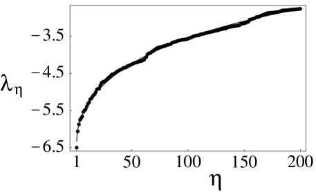
Figure 3: Dotted line is plot of $\lambda_{\eta}$ vs $\eta$ at the avoided-crossing $\tau=\tau^{*}$. It is obtained from the numerical solution of the stationary Schrödinger equation for the same instance of NPP as in Fig. 2. Solid line is a square-root fit $\lambda=-6.3+0.35\,\eta^{1/2}$ (solid line is almost undistinguishable from the dotted line).

V Simulations of time-dependent Schrödinger equation

We also study the complexity of the algorithm by numerical integration of the time-dependent Schrödinger equation with Hamiltonian $H(t)$ and initial state $|\psi(0)\rangle$ defined in Eqs. (22),(23),(27),(28). Here we relax the condition $\omega_{M}\ll\langle E\rangle$ used above in the analytical treatment of the problem; in simulations the value of $M$ is set automatically to be an integer closest to $\log_{2}\sum_{j=0}^{n}a_{j}$ (cf. (27)). We introduce a complexity metric for the algorithm, $C(T)=(1+T)d_{0}/p_{0}(T)$ where $p_{0}(t)=\sum_{{\bf w}\in{\cal L}_{0}}|\psi_{\bf w}(t)|^{2}$. A typical plot of $C(T)$ for an instance of the problem with $n$=15 numbers is shown in the insert of Fig. 4. At very small $T$ the wavefunction is close to the symmetric initial state and the complexity is $\sim 2^{n}$. The extremely sharp decrease in $C(T)$ with $T$ is due to the buildup of the population $p_{0}(T)$ in the ground level, ${\cal E}_{\bf z}=\varepsilon_{0}$, as quantum evolution approaches the adiabatic limit. At certain $T=T_{\rm min}$ the function $C(T)$ goes through the minimum: for $T>T_{\rm min}$ the decrease in the number of trials $d_{0}/p_{0}(T)$ does not compensate anymore for the overall increase in the runtime $T$ for each trial. For a given problem instance the “minimum” complexity $C_{\rm min}=C(T_{\rm min})$ is obtained via one dimensional minimization over $T$. The plot of the complexity $C_{\rm min}$ for different values of $n$ in Fig. 1 appears to indicate the exponential scaling law, $C_{\rm min}\sim 2^{0.8n}$ for not too small values of $n\gtrsim$ 11.

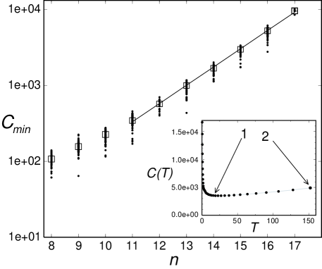
Figure 4: Logarithmic plot of $C_{\rm min}$ vs $n$ for randomly generated instances of NPP with 25-bit precision numbers. Vertical sets of points indicate results of different trials ($\sim$ 100 trials for each $n$, except $n$=17 with 10 trials). Median values of $C_{\rm min}$ are shown with rectangles. Linear fit to the logarithmic plot of median values for $n$ between 11 and 17 is shown by the line and gives $\ln C_{\rm min}\approx$ 0.55n ($C_{\rm min}\sim 2^{0.8n}$) . Very close result is obtained for the linear fit if all data points are used instead of the median values. Insert: plot of $C(T)$ vs $T$ for n=15, precision b=25 bits, $d_{0}$=22. Point $1$ indicated with the arrow refers to the minimum value of complexity at $T=T_{\rm min}=22.67$ where the total population of a ground level $p_{0}(T_{\rm min})=0.15$. Point $2$ refers to the value of $T$ where $p_{0}(T)=0.7$.

VI Discussion

In conclusion, we have developed a general method for the analysis of avoided-crossing phenomenon in quantum spin-glass problems and used it to study the performance of the quantum adiabatic evolution algorithm on random instances of the Number Partitioning problem. This algorithm is viewed as a “quantum local search” with matrix elements of the Green function $G_{r}$ ($r=1,\ldots,n-1$) giving the quantum amplitudes of the transitions with different number of spin flips $r$. Our approach is similar to the analysis of a quantum diffusion in a disordered medium with the model of disorder defined by the one- and two-point distribution functions $P(\Omega),\,P_{r,{\bf z}}(\Omega^{\prime})$.

We have shown that the conditional distribution of partition residues $P_{r}(\Omega^{\prime}|\Omega)$ in the neighborhood of a given string formed by all possible $r$-bit flips depends on the value of the partition residue for that string but not on the string itself. This is a specific property of the random Number Partitioning problem.

We used the above property to describe a quantum diffusion in the energy space (Eq. (43)). This reduction in the dimensionality leads to the formation of the eigenstate which is extended in the energy space. Near the avoided-crossing the adiabatic ground state changes from extended to mostly localized near the solution to the optimization problem. Because the extended and localized state amplitudes are nearly orthogonal to each other the repulsion between the corresponding branches of eigenvalues (the minimum gap) is exponentially small, $g_{\rm min}\sim n\,2^{-n/2}$, and the run time of the algorithm scales exponentially with $n$. Analytical results are in qualitative agreement with numerical simulations of the time-dependent Schrödinger equation for small-to-moderate instances of the Number Partitioning problem ($n\leq 17$).

One can show that the effect of quantum diffusion in reduced-dimensional space that leads to the formation of the extended state can also occur in other random NP-complete problems SST . The method developed in this paper will be applied to study the performance of continuous-time quantum algorithms for different random combinatorial optimization problems. Also the present framework can be applied to the analysis of quantum annealing algorithms for combinatorial optimization problems kadowaki ; santoro . This is a classical algorithm that is conceptually very close to the quantum adiabatic evolution algorithm considered above kadowaki1 . The former uses the Quantum Monte Carlo method to simulate on classical computers a partition function and ground-state energy of a quantum system with slowly varying Hamiltonian that merges at the final moment with the problem Hamiltonian of a given classical optimization problem. Among other possible applications of our method is the analysis of tunneling phenomenon in the low-temperature dynamics of random magnets.

We note that the specific property of the Number Partitioning problem (that distinguishes it from the other NP-complete problems) is a very weak dependence of $P_{r}(\Omega^{\prime}|\Omega)$ on $\Omega$ for not too large values of $\Omega^{\prime},\Omega\ll\sqrt{r(n-r)}$ that takes place for all values of $r\in[1,n-1]$. This rapid fall-off of correlations during the local search (both classical and quantum) is a reason that the exponential complexity of optimization algorithms for the Number Partitioning problem can be seen already for the relatively small values of $n\lesssim 15$ (cf. Fig.4).

Finally, our analysis of sub-harmonic resonances in the Fourier transform $I(s)$ of the distribution function $P(\Omega)$ suggests a possible connection between NPP and the integer factorization problem. If, for a given set of $a_{j}$’s, there is a number $q$ that satisfies the condition (64) then dividing all numbers $a_{j}$ by $q$ we obtain a new instance of NPP with numbers $k_{j}=a_{j}/q$ that will be completely equivalent to the old one. It is important that the precision of the numbers $k_{j}$ is restricted by $b-\log_{2}q$. If the value of $q$ is sufficiently large, $\log_{2}q\gg b-n$, then $k_{j}$’s correspond to a low precision instance of NPP, i.e. to the computationally easy phase mentioned in Sec. II. This is exactly the case when sub-harmonic resonances become substantial. One can fix the parameter $\xi=b/n\gg 1$ in a high-precision (computationally hard) case and compute, for randomly generated instances $\{a_{j}\}$ an approximate greatest common divider, i.e. a largest number $q$ that satisfies (64). The distribution of these numbers determines a fraction of high-precision instances of NPP (out of all possible $2^{n\,b}$ problem instances) that really belong to a low-precision (computationally easy) “phase”.

Advance knowledge of this information would be of importance if one is using NPP for encryption purposes cr , especially because NPP is otherwise a very difficult problem for both quantum and classical computers Mertens2000 . It is not obvious at this stage what the asymptotic form of this distribution will be in the limit of large $n$ (cf. Fig. A).

We are not aware of any classical algorithm that could verify if such a number $q$ exists for a given set of $a_{j}$ in a time polynomial in both $n$ and $b$. However, on a quantum computer one can apply a Shor algorithm to test in polynomial time if strong sub-harmonic resonances exist. This question is deferred to a future study.

VII Acknowledgments

The authors benefited from stimulating discussions with P. Cheeseman, R.D. Morris (NASA ARC) and U. Vazirani (UC Berkley). We also acknowledge the help of J. Lohn (Automated Design of Complex Systems group, NASA ARC) for providing computer facilities. This research was supported by NASA Intelligent Systems Revolutionary Computing Algorithms program (project No: 749-40), and also by NASA Ames NAS Center.

Appendix A Sub-harmonic resonances

We note that function $I(s)$ in (5) can also have additional sharp resonances in the range $0<|s|\leq 2^{b}$. To understand their origin we consider first a particular case when rational $b$-bit numbers $a_{1},a_{2},\ldots,a_{n}$ all have a number $q>$ 2^-b as a “common divisor”, i.e., there exist integers $k_{1},\,k_{2},\ldots,k_{n}$ such that

$$\frac{a_{1}}{k_{1}}=\frac{a_{2}}{k_{2}}=\ldots=\frac{a_{n}}{k_{n}}=q.$$ (62)

In this case additional resonances of $I(s)$ occur at the multiples of $\pi/q$. Assume now that $q$ is no longer an exact divisor of numbers $a_{j}$ but all the residues of the divisions $a_{j}/q$ are sufficiently small. Then contributions from the additional resonances at $s\approx m\pi/q$ ($m=1,\,2,\ldots$) to the integral in (5) can be estimated as follows (for simplicity we give a result for the case $E\ll n^{1/2}$):

$$P(0)\rightarrow\frac{2^{n}}{\sqrt{2\pi n\sigma^{2}(0)}}\,e^{-\gamma(q)}\,\sum_{m=1}^{\infty}\,\zeta\left(\frac{m\,\pi\eta}{2q}\right)(-1)^{mp}$$ (63)

$$p=\sum_{j=1}^{n}\left[\frac{a_{j}}{q}\right],\qquad\gamma(q)=\frac{\pi^{2}}{2}\left(\left\{\frac{a_{j}}{q}\right\}^{2}-\frac{a_{j}}{\sqrt{\pi\,n\sigma^{2}(0)}}\,\left\{\frac{a_{j}}{q}\right\}\right)$$

Here $[x]$ and $\{x\}$ denote integer and fractional parts of a number $x$, respectively. If the total “dephasing” factor $e^{-\gamma(q)}\sim 1$, then contribution (63) cannot be neglected in the steepest-descent analysis of (5) (in general, on should keep contributions from all divisors $q$ with small dephasing factors $e^{-\gamma(q)}$).

We note that the window function $\zeta\left(\frac{m\,\pi\eta}{2q}\right)\sim 1$ for $q\gg 2^{-n}$ and it decays to zero at smaller values of $q$. We studied numerically the greatest root $q_{\max}$ of the the algebraic equation

$$\gamma(q)=\gamma_{c}$$ (64)

for a fixed value of $\gamma_{c}\lesssim 1$. For the sets of random $b$-bit numbers $a_{j}$ the dependence of the mean value of $q_{\min}$ on the problem size $n<b$ is shown in Fig. 5. For $n\ll b$ we have exponential decrease of $q_{\rm max}$ with $n$ and for larger values of $n\lesssim b$ the value of $q_{\min}$ steeply drops to 1. According to the discussion above, in order to neglect the saddle-points with $s>0$ in (5) (additional resonances) the value of $q_{\min}$ should satisfy the following condition in the asymptotic limit $b\rightarrow\infty$:

$$q_{\rm max}\lesssim\max\left[2^{-n},2^{-b}\right],\qquad 1\ll n\ll b,$$ (65)

with $\gamma_{c}$ fixed at some small constant value. Because the precision $b$ that we used in the simulations was not very high (limited by machine precision) it is not possible to obtain the asymptotic form of the dependence of $q_{\min}$ on $n$ in the range given in (65). Neither we can describe the shape of the plot in Fig. 5 analytically in that range. However, it appears from the figure that the condition (65) is satisfied for sufficiently large $n$.

Figure 5: Log-Log plots of the mean value of the largest root of Eq. (64) $q_{\min}$ vs $n$. Three sets of data points are plotted. Each set of points represents averaging over 25 randomly generated instances of NPP. Precision of the random numbers $a_{j}$ is 30 bits and the value of $\gamma_{c}=0.5$. Dashed line corresponds to the plot of $const\times 2^{-n}$ vs $n$. Insert: Variance of the $\log_{2}q$ vs $n$ based on 25 sample points for each $n$. Distribution of $q_{\min}$ values become very broad when the mean drops to $q_{\min}\sim 1$.

Appendix B Properties of the conditional distribution of signed residues in NPP

We perform the summation over the spin configurations in Eq. (17) with Eq. (15) taken into account. Similar to the derivation of Eq. (5) we use integral representation for delta function and obtain

$$P_{r}(\Omega,\Omega^{\prime})=\binom{n}{r}^{-1}\,\int_{-\infty}^{\infty}\int_{-\infty}^{\infty}\frac{ds\,ds^{\prime}}{4\pi^{2}}\,\zeta\left(\frac{\Delta\Omega s}{2}\right)\,\zeta\left(\frac{\Delta\Omega^{\prime}s^{\prime}}{2}\right)\,\,\sum_{{\bf J}}U_{\bf J}(s,s^{\prime}),$$ (66)

$$U_{\bf J}(s,s^{\prime})=\prod_{j\in{\bf J}}\cos(a_{j}(s-s^{\prime}))\,\times\,\prod_{j\notin{\bf J}}\cos(a_{j}(s+s^{\prime}))\,\times\,e^{i(s\,\Omega+s^{\prime}\,\Omega^{\prime})}.$$

Here the sum is over all possible subsets ${\bf J}=\{j_{1},j_{2},\ldots,j_{r}\}$ of length $r$ obtained from the set of integers $j=1,2,\ldots,n$. Window function $\zeta(x)$ is defined in (5). After the change of variables

$$x^{\prime}=s+s^{\prime},\qquad x=s-s^{\prime},$$ (67)

we obtain from (66) that $U_{\bf J}(s,s^{\prime})$ factorizes into a product of two terms

$$U_{\bf J}(s,s^{\prime})\,=\,{\cal V}_{\bf J}(x)\,\widetilde{\cal V}_{\bf J}(x^{\prime})$$

$${\cal V}_{\bf J}(x)=\exp\left(\frac{ix(\Omega-\Omega^{\prime})}{2}\right)\prod_{j\in{\bf J}}\cos(a_{j}\,x),\quad\widetilde{\cal V}_{\bf J}(x^{\prime})=\exp\left(\frac{ix^{\prime}(\Omega+\Omega^{\prime})}{2}\right)\prod_{j\notin{\bf J}}\cos(a_{j}\,x^{\prime}).$$ (68)

In what follows we will analyze several limiting cases.
$r,n-r\gg 1$:
In this case both functions ${\cal V}_{\bf J}(x)$ and $\widetilde{\cal V}_{\bf J}(x^{\prime})$ are very steep and similar to the analysis in Sec.II.1 integrals in (66) can be evaluated by the steepest descent method. With the appropriate choice of the coarse-graining windows $\Delta\Omega,\,\Delta\Omega^{\prime}$ in (66) (see below) contribution to the integrals comes from the vicinity of the point ($x=0,x^{\prime}=0$). Near this point we use

$$\prod_{j\in{\bf J}}\cos(a_{j}\,x)\approx\exp\left(-\frac{r(x\,\sigma_{\bf J})^{2}}{2}\right),\qquad\prod_{j\notin{\bf J}}\cos(a_{j}\,x)\approx\exp\left(-\frac{(n-r)(x^{\prime}\,\overline{\sigma}_{\bf J})^{2}}{2}\right)$$ (69)

where

$$(\sigma_{\bf J})^{2}=\frac{1}{r}\sum_{j\in{\bf J}}a_{j}^{2},\qquad(\overline{\sigma}_{\bf J})^{2}=\frac{1}{n-r}\sum_{j\notin{\bf J}}a_{j}^{2}.$$

Since each sum here contains a large number of terms we obtain for i.i.d. random numbers $a_{1},\ldots,a_{n}$ (cf. (6))

$$(\sigma_{\bf J})^{2}\approx\sigma^{2}(0)+{\cal O}\left(\frac{1}{r}\right),\qquad(\overline{\sigma}_{\bf J})^{2}\approx\sigma^{2}(0)+{\cal O}\left(\frac{1}{n-r}\right),$$ (70)

where $\sigma^{2}=\langle a^{2}\rangle$ is given in (6). Using Eqs. (68)-(70) and replacing the window functions in (66) by unity, we compute the Gaussian integrals in (66) and obtain

$$P_{r}(\Omega,\Omega^{\prime})=\frac{1}{4\pi\sigma^{2}(0)\sqrt{r(n-r)}}\exp\left[-\frac{1}{8\sigma^{2}(0)}\left(\frac{(\Omega-\Omega^{\prime})^{2}}{r}+\frac{(\Omega+\Omega^{\prime})^{2}}{n-r}\right)\right].$$ (71)

The size of the coarse-graining windows in (66) is chosen to satisfy the conditions

$$2^{-n}\,\binom{n}{r}^{-1}\ll\Delta\Omega\,\Delta\Omega^{\prime}\ll\sqrt{r(n-r)}$$

From Eq. (71) and Eq. (6) one can directly obtain the conditional distribution function $P_{r}(\Omega|\Omega^{\prime})$

$$P_{r}(\Omega^{\prime}|\Omega)=\frac{1}{\sqrt{2\pi n\sigma^{2}(q)}}\exp\left[-\frac{\left(\Omega^{\prime}-q\,\Omega\right)^{2}}{2n\sigma^{2}(q)}\right].$$ (72)

$r=1$; $\quad r=n-1$:
For $r=1$ function $\overline{{\cal V}}_{\bf J}(x^{\prime})$ contains a product of $n-1$ terms and is very steep. The corresponding integral over $x^{\prime}$ in (66) should be taken by the steepest descent method. However ${\cal V}_{\bf J}(x)$ simply oscillates at frequencies $(\Omega-\Omega^{\prime})/2\pm a_{j}$ and the integral over $x$ in (66) should be evaluated using the corresponding oscillating factors. In the opposite case $r=n-1$, function ${\cal V}_{\bf J}(x)$ is very steep and the integral over $x$ in (66) should be taken by steepest descent. But the integral over $x^{\prime}$ there should be evaluated using $\overline{{\cal V}}_{\bf J}(x^{\prime})$ that oscillates at the frequencies, $(\Omega+\Omega^{\prime})/2\pm a_{j}$. Finally, one can obtain using i.i.d. numbers $a_{j}$’s in $\left[0,1\right]$ interval :

$$P_{r}(\Omega^{\prime}|\Omega)=\frac{1}{4}\left[\Theta\left(\Omega\mp\Omega^{\prime}+2\right)-\Theta\left(\Omega\mp\Omega^{\prime}-2\right)\right]+{\cal O}\left(\frac{1}{n}\right),\qquad(r=1,\,n-1).$$ (73)

The minus (plus) sign in (73) corresponds to $r=1$ ($r=n-1$). Similarly one can obtain the result for any fixed value of $r$ or $n-r$ (that does not scale with $n$). For $|\Omega|,|\Omega^{\prime}|\lesssim 1$ (73) is reduced to (19).

Numerical simulations of conditional distribution $P_{r,{\bf z}}(\Omega^{\prime})$

We compute the following integrated quantity:

$$Q=\frac{1}{2}\,\int_{0}^{\Omega^{\prime}}d\eta\,P_{r,{\bf z}}(\eta),$$ (74)

for different values of $r$, $\Omega^{\prime}$ and different strings ${\bf z}$ with $E_{\bf z}\ll 1$. Numerical results are compared in the insert to Fig.1 with theoretical result below obtained using $P_{r}(\Omega^{\prime}|\Omega)$ from Eq. (72)

$$\frac{1}{2}\int_{0}^{\Omega^{\prime}}d\eta\,P_{r}(\eta|0)={\rm erf}\left(\frac{\Omega^{\prime}}{\sigma(q)\,\sqrt{2n}}\right).$$ (75)

Theoretical and numerical curves nearly coincide with each other. To accurately compare the normalization factor in (72) (see also (20)) we compare the theoretical results with numerical values of $P_{r,{\bf z}}(0)$ for different $r$ and strings ${\bf z}$ corresponding to $E_{\bf z}\ll 1$. The results are plotted in Fig. 1.

References

- (1) P.W. Shor, in Proceedings of the 35th Annual Symposium on the Foundations of Computer Science, ed. by S. Goldwasser (IEEE Computer Society Press, Los Alamitos, CA, 1994), p.124; SIAM J. Comput. 26, p.1484 (1997).
- (2) Y. Fu and P.W. Anderson, J. Phys. A: Math. Gen. 19, 1605-1620 (1986).
- (3) M. Mezard, G. Parizi, and M. Virasoro, Spin glass theory and beyond (World Scientific, Singapore, 1987).
- (4) M.R. Garey and D.S. Johnson, Computers and Intractability. A Guide to the Theory of NP-Completeness (W.H. Freeman, New York, 1997)
- (5) E. Farhi, J. Goldstone, S. Gutmann, and M. Sipser, arXiv:quant-ph/0001106.
- (6) E. Farhi, J. Goldstone, S. Gutmann, J. Lapan, A. Lundgren, and D. Preda, Science 292, 472 (2001).
- (7) E. Farhi, J. Goldstone, and S. Gutmann, arXiv:quant-ph/0007071.
- (8) A. M. Childs, E. Farhi, J. Goldstone, and S. Gutmann, arXiv:quant-ph/0012104.
- (9) T.Hogg, “Adiabatic Quantum Computing for Random Satisfiability Problems”, arXiv:quant-ph/0206059.
- (10) W. Van Dam, M. Mosca, U. Vazirani, ”How Powerful is adiabatic Quantum Computation?”, arXiv:quant-ph/0206003.
- (11) C. Bennett, E. Bernstein, G. Brassard, and U. Vazirani, ”Sterngths and weaknesses of quantum computing”, SIAM Journal of Computing, 26, pp. 1510-1523 (1997); arXiv:quant-ph/9701001.
- (12) W. Van Dam, M. Mosca, U. Vazirani, ”How Powerful is Idiabatic Quantum Computation?”, FOCS 2001.
- (13) E. Farhi, J. Goldstone, S. Gutmann, arXiv:quant-ph/0201031.
- (14) A. M. Childs, E. Deotto, E. Farhi, J. Goldstone, S. Gutmann, A. J. Landhal, “Quantum search by measurment”, arXiv:quant-ph/0204013.
- (15) A. Boulatov, V. Smelyanskiy, “Total suppression of a large spin tunneling barrier in quantum adiabatic computation”, arXiv:quant-ph/0208189.
- (16) Li-Hui Tsai, SIAM J. Comput., 21(1) p.59-64 (1992).
- (17) A. Shamir, Proc. of 11th Annual ACM Symposium on Theory of Computing, p.118 (1979).
- (18) N. Karmakar, R.M. Karp, G.S. Lueker, and A.M. Odlyzko, J. App. Prob. 23, p. 626 (1986).
- (19) D.S. Johnson, et al., Operations Research 39, p.378 (1991).
- (20) F.F. Ferreira and J. F. Fontanari, J. Phys. A 31, p. 3417 (1998).
- (21) I.P. Gent and T. Walsh, in Proc. of the ECAI-96, ed. by W. Wahlster (John-Wiley Sons, New York, 1996), pp. 170-174.
- (22) R.E. Korf, Artificial Intelligence 106, 181 (1998).
- (23) S. Mertens, Phys. Rev.Lett. 81, 4281–4284 (1998).
- (24) C. Borgs, J. T. Chayes and B. Pittel, Proc. of the 2001 ACM Symposium on the Theory of Computing, pp. 330-336 (2001).
- (25) C. Borgs, J. T. Chayes and B. Pittel, Random Structures and Algorithms, v. 19, pp. 247-288 (2001)
- (26) S. Mertens, ”A complete anytime algorithm for balanced partitioning”arXiv:abs/cs.DS/9903011.
- (27) P. Cheeseman, B. Kanefsky and W. M. Taylor, Proc. of the International Joint conference on Artificial Intelligence, v. 1, pp. 331-337 (1991).
- (28) Artif. Intel. 81 (1-2) (1996), special issue on Topic, ed. by T. Hogg, B.A. Huberman, and C. Williams.
- (29) S. Mertens, Phys. Rev.Lett. 84, 1347–1350 (2000).
- (30) S. Lloyd, Science 273, 1073 (1996).
- (31) V. Smelyanskiy, D. Shumow, U. Toussaint, in preparation.
- (32) T. Kadowaki and N. Nishimori, Phys. Rev. E 58, p. 5355 (1998).
- (33) G. Santoro, R. Martonak, E. Tosatti, R. Car, Science 295, p. 2427 (2002).
- (34) T. Kadowaki, “Study of Optimization problems by quantum annealing”, PhD Thesis, arXiv:quant-ph/020520 (2002).