Universal measurement apparatus controlled by quantum software

Abstract

We propose a quantum device that can approximate any projective measurement on a qubit. The desired measurement basis is selected by the quantum state of a “program register”. The device is optimized with respect to maximal average fidelity (assuming uniform distribution of measurement bases). An interesting result is that if one uses two qubits in the same state as a program the average fidelity is higher than if he/she takes the second program qubit in the orthogonal state (with respect to the first one). The average information obtainable by the proposed measurements is also calculated and it is shown that it can get different values even if the average fidelity stays constant. Possible experimental realization of the simplest proposed device is presented.

Programmable quantum “multimeters” are devices that can realize any desired generalized quantum measurement from a chosen set (either exactly or approximately) DuBu . Their main feature is that the particular positive operator valued measure (POVM) is selected by the quantum state of a “program register” (quantum software). In this sense they are analogous to universal quantum processors Nielsen97 ; Vidal00 ; Hillery02 . Quantum multimeters could play an important role in quantum state estimation and quantum information processing.

In this paper, we will describe a programable quantum device that can approximately accomplish any projective von Neumann measurement on a single qubit. Since it is impossible to encode an arbitrary unitary operation (acting on a finite-dimensional Hilbert space) into a state of a finite-dimensional quantum system Nielsen97 it is also impossible to encode arbitrary projective measurement on a qubit into such a state DuBu . However, it is still possible to encode POVM’s that represent, in a certain sense, the best approximation of the required projective measurements.

Suppose we would like to measure a qubit in the basis represented by two orthogonal vectors $|\psi\rangle$ and $|\psi_{\perp}\rangle$. We want this measurement basis be controlled by the quantum state of a program register, $|\phi_{p}(\psi)\rangle$. An ideal multimeter would map the composite state of the measured system and the program register to two fixed orthogonal pure states $|0\rangle$ and $|1\rangle$ according to

$$|\psi\rangle\otimes|\phi_{\rm p}(\psi)\rangle\rightarrow|0\rangle,\qquad|\psi_{\perp}\rangle\otimes|\phi_{\rm p}(\psi)\rangle\rightarrow|1\rangle.$$ (1)

As mentioned above, such transformation cannot be implemented exactly. Thus, our task is to find a realistic linear trace-preserving completely positive (CP) map that represents the closest approximation to this non-realistic map. We focus on the scenario when we always obtain one of the two measurement results $|0\rangle$ or $|1\rangle$ but errors, i.e. deviations from the ideal map (1), may appear. Our aim is to minimize the probability of error, i.e., we will maximize the probability of the correct discrimination between states $|\psi\rangle$ and $|\psi_{\perp}\rangle$. In general we could optimize both the program and the fixed transformation so as to optimally approximate map (1) for a given dimension of the program register. However, this is an extremely hard problem that we will not attempt to solve in its generality. Instead, we shall optimize the fixed transformation for two natural choices of the program.

First we shall assume that the program register contains $N$ copies of the state $|\psi\rangle$, $|\phi_{\rm p}(\psi)\rangle=|\psi\rangle^{\otimes N}$. Our second choice of the program – the two-qubit state $|\psi\rangle|\psi_{\perp}\rangle$ – is motivated by recent results on optimum quantum state estimation. Gisin and Popescu showed that the state of two orthogonal qubits $|\psi\rangle|\psi_{\perp}\rangle$ encodes the information on the state $|\psi\rangle$ better than state of two identical qubits $|\psi\rangle|\psi\rangle$ Gisin99 . If we possess one copy of the state $|\psi\rangle|\psi_{\perp}\rangle$ than we can estimate $|\psi\rangle$ with fidelity ${\cal{F}}_{\perp}=(1+1/\sqrt{3})/2\approx 0.7886$ which is slightly higher than the fidelity of optimum estimation on one copy of two identical qubits, ${\cal{F}}_{||}=3/4$ Gisin99 ; Massar00 . One would thus expect that the state $|\psi\rangle|\psi_{\perp}\rangle$ should also give an advantage when used as a program of the multimeter. Rather surprisingly, this is not the case and we shall see that it is better to use two identical qubits $|\psi\rangle|\psi\rangle$.

In what follows we shall benefit from the isomorphism between CP maps and bipartite positive semidefinite operators Jamiolkowski72 ; Fiurasek01 . Let $\cal{H}$ and $\cal{K}$ denote the Hilbert spaces of input and output states, respectively. Choose basis $|i\rangle$ in $\cal{H}$, define a maximally entangled state $\sum_{i}|i\rangle|i\rangle$ on ${\cal{H}}^{\otimes 2}$ and apply the CP map to one part of this state. The density matrix $\chi$ of the resulting state on Hilbert space ${\cal{H}}\otimes\cal{K}$ represents the CP map and the relation between input and output density matrices reads Fiurasek01

$$\rho_{\rm out}={\rm Tr}_{\rm in}[\chi\rho_{\rm in}^{T}\otimes\openone_{\rm out}]$$ (2)

where $T$ stands for the transposition in the basis $|i\rangle$ and $\openone$ denotes an identity operator. The CP map is trace preserving if the positive semidefinite operator $\chi$ satisfies the condition ${\rm Tr}_{\rm out}[\chi]=\openone_{\rm in}$.

Let us define the fidelity $F(\psi)$ of our multimeter projecting onto states $|\psi\rangle$ and $|\psi_{\perp}\rangle$ as the probability that a correct measurement result will be obtained when we send the states $|\psi\rangle$ or $|\psi_{\perp}\rangle$ to the input randomly each with probability one half. This probability can be interpreted as a success rate of the discrimination between two orthogonal states $|\psi\rangle$ and $|\psi_{\perp}\rangle$. Assuming the program state to be $|\psi\rangle^{\otimes N}$, the two relevant input states of the multimeter read

$$|\Psi\rangle=|\psi\rangle\otimes|\psi\rangle^{\otimes N},\qquad|\Psi_{\perp}\rangle=|\psi_{\perp}\rangle\otimes|\psi\rangle^{\otimes N}.$$ (3)

The input Hilbert space of the multimeter is a tensor product of the Hilbert space of signal qubit ${\cal{H}}_{\rm s}$ and symmetric (bosonic) subspace ${\cal{H}}_{+}^{N}$ of the Hilbert space of $N$ qubits, ${\cal{H}}={\cal{H}}_{\rm s}\otimes{\cal{H}}_{+}^{N}$ and ${\rm dim}{\cal{H}}=2(N+1)$. A trace preserving completely positive map $\chi$ transforms the input states onto the states of a single output qubit that is subsequently measured in the computational basis. The outcome $|0\rangle$ corresponds to the projection onto $|\psi\rangle$ while $|1\rangle$ is associated with the projection onto $|\psi_{\perp}\rangle$. Making use of the input-output relation (2) we have,

$$F(\psi) = \frac{1}{2}{\rm Tr}\Bigl{[}\chi(|\Psi\rangle\langle\Psi|)^{T}\otimes|0\rangle\langle 0|\Bigr{]}$$ (4)

$$+ \frac{1}{2}{\rm Tr}\Bigl{[}\chi\,(|\Psi_{\perp}\rangle\langle\Psi_{\perp}|)^{T}\otimes|1\rangle\langle 1|\Bigr{]}.$$

The figure of merit that we would like to maximize is the mean fidelity obtained on averaging $F(\psi)$ over all pure qubit states $|\psi\rangle$, i.e., over the surface of the Bloch sphere,

$$F=\int_{\psi}d\psi\,F(\psi)=\rm Tr[R\chi].$$ (5)

The positive semidefinite operator $R$ reads

$$R=R_{+}\otimes|0\rangle\langle 0|+R_{-}\otimes|1\rangle\langle 1|,$$ (6)

where the operators $R_{+}$ and $R_{-}$ acting on the input Hilbert space $\cal{H}$ are given by integrals

$$R_{+}^{T}=\frac{1}{2}\int_{\psi}d\psi\,|\Psi\rangle\langle\Psi|,\qquad R_{-}^{T}=\frac{1}{2}\int_{\psi}d\psi\,|\Psi_{\perp}\rangle\langle\Psi_{\perp}|.$$ (7)

A straightforward calculation reveals that $R_{+}$ is proportional to the projector onto symmetric subspace ${\cal{H}}_{+}^{(N+1)}$ of the Hilbert space of $N+1$ qubits,

$$R_{+}=\frac{1}{2(N+2)}\Pi_{+}^{(N+1)}.$$ (8)

Furthermore, the sum of operators $R_{+}$ and $R_{-}$ is proportional to the identity operator on the input Hilbert space, $R_{+}+R_{-}=\openone_{\rm in}/[2(N+1)]$. Thus we immediately have

$$R_{-}=\frac{1}{2(N+1)}\openone_{\rm in}-\frac{1}{2(N+2)}\Pi_{+}^{(N+1)}.$$ (9)

The determination of the optimum CP map amounts to maximization of the linear function (5) under the constraints $\chi\geq 0$ and ${\rm Tr}_{\rm out}[\chi]=\openone_{\rm in}$. The optimum CP map that maximizes the mean fidelity (5) must satisfy the extremal equations Fiurasek01 ; Audenaert01

$$(\lambda\otimes\openone_{\rm out}-R)\chi=0,$$ (10)

$$\lambda\otimes\openone_{\rm out}-R\geq 0,\quad$$ (11)

where $\lambda$ is positive definite operator on the input Hilbert space. Notice that the extremal equations (10) and (11) resemble the Helstrom equations for optimum POVM that maximizes the success rate in ambiguous quantum state discrimination helst . One can prove that if both Eqs. (10) and (11) are satisfied, then $\chi$ is indeed optimum CP map and $F$ attains its global maximum on the convex set of trace-preserving CP maps Audenaert01 ; Fiurasek01b .

The extremal equations can be very efficiently solved numerically by means of repeated iterations Fiurasek01 . From the numerical results, we were able to conjecture the optimum CP map,

$$\chi=\Pi_{+}^{(N+1)}\otimes|0\rangle\langle 0|+\Pi_{-}^{(N+1)}\otimes|1\rangle\langle 1|.$$ (12)

where $\Pi_{-}^{(N+1)}=\openone_{\rm in}-\Pi_{+}^{(N+1)}$ is a projector onto subspace orthogonal to the symmetric subspace of $N+1$ qubits. On inserting the expressions (6) and (12) into Eq. (5), we obtain the mean fidelity

$$F=\frac{2N+1}{2N+2}.$$ (13)

Prior to analyzing the properties of the CP map (12) in detail, let us prove its optimality. Taking into account the trace-preservation condition ${\rm Tr}_{\rm out}[\chi]=\openone_{\rm in}$, we find from Eq. (10) that $\lambda={\rm Tr}_{\rm out}[R\chi]$. After some algebra we arrive at

$$\lambda=\frac{1}{2(N+1)}\openone_{\rm in}-\frac{1}{2(N+1)(N+2)}\Pi_{+}^{(N+1)}.$$ (14)

It is easy to check that the first extremal equation (10) is satisfied. The inequality (11) splits into two independent inequalities for operators acting on input Hilbert space,

$$A_{1}=\lambda-R_{-}\geq 0,\qquad A_{2}=\lambda-R_{+}\geq 0.$$

A straightforward calculation yields explicit formulas for $A_{1}$ and $A_{2}$,

$$A_{1} = \frac{N}{2(N+1)(N+2)}\,\Pi_{+}^{(N+1)},$$

$$A_{2} = \frac{1}{2(N+1)}\,\Pi_{-}^{(N+1)}.$$ (15)

Since both these operators are positive semidefinite, the condition (11) is satisfied. This concludes our proof of the optimality of the CP map (12).

The structure of the optimum CP map (12) indicates that this map is a joint generalized quantum measurement on the signal qubit and $N$ program qubits and the corresponding POVM has two elements $\Pi_{+}^{(N+1)}$ and $\Pi_{-}^{(N+1)}$. We can now determine the effective POVM carried out on the signal qubit,

$$\Pi_{||} = {\rm Tr}_{\rm p}\left[\openone_{\rm s}\otimes(|\psi\rangle\langle\psi|)^{\otimes N}\,\Pi_{+}^{(N+1)}\right],$$

$$\Pi_{\perp} = {\rm Tr}_{\rm p}\left[\openone_{\rm s}\otimes(|\psi\rangle\langle\psi|)^{\otimes N}\,\Pi_{-}^{(N+1)}\right],$$ (16)

where ${\rm Tr}_{\rm p}$ denotes trace over the program qubits. The outcome $\Pi_{\perp}$ cannot occur if the input state is $|\psi\rangle$ because the input state $|\Psi\rangle$ belongs to the symmetric subspace of $N+1$ qubits and $\Pi_{||}$ clicks with certainty. Hence the POVM element $\Pi_{\perp}$ must be proportional to the projector $|\psi_{\perp}\rangle\langle\psi_{\perp}|$. Since the sum of POVM elements (16) is an identity operator, we have the following ansatz,

$$\Pi_{||} = |\psi\rangle\langle\psi|+(1-p)|\psi_{\perp}\rangle\langle\psi_{\perp}|,$$

$$\Pi_{\perp} = p\,|\psi_{\perp}\rangle\langle\psi_{\perp}|.$$ (17)

The probability $p$ that $\Pi_{\perp}$ clicks when the input state is $|\psi_{\perp}\rangle$ is given by $p=\langle\Psi_{\perp}|\Pi_{-}^{(N+1)}|\Psi_{\perp}\rangle$. After some algebra we get $p=N/(N+1)$ and the effective POVM representing our universal multimeter reads

$$\Pi_{||} = \frac{1}{N+1}\openone+\frac{N}{N+1}|\psi\rangle\langle\psi|,$$

$$\Pi_{\perp} = \frac{N}{N+1}|\psi_{\perp}\rangle\langle\psi_{\perp}|.$$ (18)

Notice that the POVM (18) is asymmetric, which reflects the asymmetry of the program register. Furthermore, the fidelity $F(\psi)$ is independent of $\psi$ and equal to the mean fidelity (13). In the limit of infinitely large program register $(N\rightarrow\infty)$, the POVM (18) approaches the ideal projective measurement.

We now turn our attention to the program $|\psi\rangle|\psi_{\perp}\rangle$. The optimum CP map for this program can be found following the same procedure as described above for the program $|\psi\rangle^{\otimes N}$. Briefly, one has to calculate the operator $R$ and solve extremal equations (10) and (11). We will not give the details of calculations here and only present the results. Similarly as before, the optimum CP map is a generalized measurement on the signal qubit and two program qubits. The two elements of this three-qubit POVM read,

$$\Pi_{+} = \frac{1}{2}\Pi_{+}^{(3)}+|\phi_{1}\rangle\langle\phi_{1}|+|\phi_{2}\rangle\langle\phi_{2}|,$$

$$\Pi_{-} = \openone_{3}-\Pi_{+},$$ (19)

where $\openone_{3}$ is an identity operator on Hilbert space of three qubits and

$$|\phi_{1}\rangle = \frac{1}{2\sqrt{3}}[(\sqrt{3}+1)|0\rangle_{\rm s}|01\rangle_{\rm p}-(\sqrt{3}-1)|0\rangle_{\rm s}|10\rangle_{\rm p}$$

$$-2\,|1\rangle_{\rm s}|00\rangle_{\rm p}],$$

$$|\phi_{2}\rangle = \frac{1}{2\sqrt{3}}[(\sqrt{3}+1)|1\rangle_{\rm s}|10\rangle_{\rm p}-(\sqrt{3}-1)|1\rangle_{\rm s}|01\rangle_{\rm p}$$ (20)

$$-2\,|0\rangle_{\rm s}|11\rangle_{\rm p}].$$

Here the subscripts s and p label the states of signal and program qubits, respectively. After some algebra, we find the effective POVM carried out on the signal qubit,

$$\Pi_{||}^{\prime} = \frac{3-\sqrt{3}}{6}\openone+\frac{\sqrt{3}}{3}|\psi\rangle\langle\psi|,$$

$$\Pi_{\perp}^{\prime} = \frac{3-\sqrt{3}}{6}\openone+\frac{\sqrt{3}}{3}|\psi_{\perp}\rangle\langle\psi_{\perp}|.$$ (21)

This POVM is symmetric (reflecting the symmetry of the program $|\psi\rangle|\psi_{\perp}\rangle$). The fidelity $F(\psi)$ is state independent and equal to the mean fidelity

$$F^{\prime}=\frac{1}{2}\left(1+\frac{1}{\sqrt{3}}\right).$$ (22)

Notice that $F^{\prime}={\cal{F}}_{\perp}$. This is not a mere coincidence, the optimum strategy for program $|\psi\rangle|\psi_{\perp}\rangle$ is to carry out an optimal estimation of $|\psi\rangle$ and then measure the signal qubit in the basis formed by estimated state $|\psi_{\rm est}\rangle$ and its orthogonal counterpart. The POVM (19) is an explicit implementation of this procedure. We emphasize here that $F^{\prime}$ is a maximum fidelity attainable with program $|\psi\rangle|\psi_{\perp}\rangle$, because the corresponding CP map solves the extremal equations (10) and (11). With the program $|\psi\rangle|\psi\rangle$ we achieve the fidelity $5/6\approx 0.8333$ which is higher than $F^{\prime}$, hence the program $|\psi\rangle|\psi\rangle$ exhibits better performance than $|\psi\rangle|\psi_{\perp}\rangle$.

The aim of the measurement is to obtain some information on the system. It can be illustrated on the following example: Alice encodes bits of a message into quantum states and Bob tries to read the message making measurements on these states. The average Bob’s information (per bit) on the message can be quantified as

$$I=\sum_{i}r_{i}\left[1+p_{i}\log_{2}p_{i}+(1-p_{i})\log_{2}(1-p_{i})\right],$$ (23)

where $r_{i}$ is a fraction of bits that Bob knows with probability $p_{i}$ ($\sum_{i}r_{i}=1$). It is reasonable to look for measurements that maximize average information per . However, as the average information is a non-linear function of probabilities this is usually a very difficult problem. We will not try to search for a CP map (or POVM) that would maximize information instead of fidelity. Nevertheless, we will calculate the average information obtainable by the measurements described above that are optimal with respect to the fidelity. Let us define fidelities $F_{||}=\langle\psi|\Pi_{||}|\psi\rangle$ and $F_{\perp}=\langle\psi_{\perp}|\Pi_{\perp}|\psi_{\perp}\rangle$. If the average rates of both the states are the same and equal to $1/2$ (generalization to an arbitrary rate is straightforward) then

$$r_{||}=\left[F_{||}+(1-F_{\perp})\right]/2,\quad p_{||}=F_{||}/(2r_{||}),$$

$$r_{\perp}=\left[F_{\perp}+(1-F_{||})\right]/2,\quad p_{\perp}=F_{\perp}/(2r_{\perp}).$$ (24)

For example, if $F_{||}=1$ and $F_{\perp}=1/2$ Bob gets result “0” always when Alice sends $|\psi\rangle$ and in half cases when she sends $|\psi_{\perp}\rangle$. So, he knows the original bit with probability $p_{||}=2/3$ and the average relative number of these results is $r_{||}=3/4$. For result “1” the probability $p_{\perp}=1$ (this result appears only if Alice sends $|\psi_{\perp}\rangle$) and $r_{\perp}=1/4$. This leads to average information $I\doteq 0.311$. The described situation corresponds to the above mentioned measurement with the program state $|\psi\rangle$. Note that a symmetrized measurement with the same average fidelity ($F_{||}=F_{\perp}=3/4$) would lead to lower information ($I\doteq 0.189$).

For the case when the program state is $|\psi\rangle|\psi\rangle$ and $F_{||}=1$, $F_{\perp}=2/3$ the average information gets value $I\doteq 0.459$. For the program state $|\psi\rangle|\psi_{\perp}\rangle$, when $F_{||}=F_{\perp}=\frac{1}{2}(1+\frac{1}{\sqrt{3}})$, the information is $I\doteq 0.256$. Notice that this information is lower than the one obtained with the device programmed by the single-qubit program state $|\psi\rangle$ ($0.256<0.311$).

Figure 1: Quantum circuit representing simple programmable multimeter: H – Hadamard gate, F – Fredkin gate.

The proposed universal measurement devices can be, at least in principle, realized experimentally. As an example, we describe now a possible realization of the simplest one that uses a single-qubit program register. Such a device can be built up from one Fredkin (controlled swap) and two Hadamard gates as shown in Fig. 1 Ekert01 . Signal and program enter the Fredkin gate as “controlled” qubits; the result can be read out from the ancilla serving as a “control” qubit. There are several ways how to implement the presented scheme on real physical systems radim . For example, we can employ an experimental setup suggested previously in cavity-QED experiments Raimond97 that is sketched in Fig. 2. The Fredkin gate is realized by two cavities C₀ and C₁ coupled by a waveguide and it is controlled by an atomic “probe” affecting cavity field through a nonlinear atom-field interaction in a large-detuning limit Brune92 . This gate is inserted between two Hadamard gates implemented as Ramsey atomic interferometers. The state of cavity C₁ represents the signal, the state of cavity C₀ the program. The program state can be set employing an atom-field interaction too. An atom is prepared in the desired program state $a|{\rm g}\rangle+b|{\rm e}\rangle$. This is done in zones B and R₁ (atoms come from an oven O and only those with an appropriate velocity are selected in zone V). An atom transition frequency must coincide with the cavity frequency. Passing through the cavity C₀ the atom changes its photonic state to $a|0\rangle+b|1\rangle$. Once the program and the signal are encoded into the states of the cavities, 50:50 coupling between C₀ and C₁ is established. Then the second atom, initially prepared in the excited state, is sent through the Ramsey interferometer. This atom is exposed to the nonlinear interaction with the cavity field in a large-detuning limit (in contrast to the first one). Finally, the result of our programmed measurement process encoded in the state of the atom can be revealed by the field-ionization counters D_e end D_g.

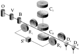
Figure 2: Experimental realization of a programmable multimeter in cavity QED: O – oven, V – velocity selection, B – excitation box, R₁, R₂ – Ramsey zones, C₀, C₁ – high-Q cavities, S^′ – microwave source, D_e, D_g – ionization detectors.

- (1) M. Dušek and V. Bužek, quant-ph/0201097.
- (2) M. A. Nielsen and I. L. Chuang, Phys. Rev. Lett. 79, 321 (1997).
- (3) G. Vidal and J. I. Cirac, quant-ph/0012067.
- (4) M. Hillery, V. Bužek, and M. Ziman, Phys. Rev. A 65, 022301 (2002).
- (5) N. Gisin and S. Popescu, Phys. Rev. Lett. 83, 432 (1999).
- (6) S. Massar, Phys. Rev. A 62, 040101(R) (2000).
- (7) A. Jamiołkowski, Rep. Math. Phys. 3, 275 (1972).
- (8) J. Fiurášek, Phys. Rev. A 64, 062310 (2001).
- (9) K. Audenaert and B. De Moor, Phys. Rev. A 65, 030302(R) (2002).
- (10) C. W. Helstrom, Quantum Detection and Estimation Theory (Academic Press, New York, 1976).
- (11) J. Fiurášek, S. Iblisdir, S. Massar, and N.J. Cerf, quant-ph/0110016.
- (12) A. Peres, Quantum Theory: Concepts and Methods (Kluwer, Dordrecht, 1993).
- (13) A.K. Ekert, C.M. Alves, D.K.L. Oi, M. Horodecki, P. Horodecki, and L.C. Kwek, quant-ph/0112073.
- (14) R. Filip, quant-ph/0108119.
- (15) J. M. Raimond, M. Brune, and S. Haroche, Phys. Rev. Lett. 79, 1964 (1997).
- (16) M. Brune, S. Haroche, J. M. Raimond, L. Davidovich, and N. Zagury, Phys. Rev. A 45, 5193 (1992).