Entanglement of Distillation
and Conditional Mutual Information

Abstract

In previous papers, we expressed the Entanglement of Formation in terms of Conditional Mutual Information (CMI). In this brief paper, we express the Entanglement of Distillation in terms of CMI.

1 Introduction

Entanglement of Formation ($E_{F}$) and Entanglement of Distillation ($E_{D}$) were invented by Bennett et al in Ref.[1] and satellite papers. In a series of previous papers[2], we showed how to express $E_{F}$ in terms of Conditional Mutual Information (CMI), but we said nothing about $E_{D}$. In this brief letter, we will show how to express $E_{D}$ in terms of CMI. Recently, other researchers have expressed some of their entanglement ideas in terms of unconditional mutual information. See, for example, Ref.[3].

Two reasons why CMI is useful for quantifying entanglement are the following. First, entanglement is an “exclusively quantum” effect. CMI satisfies this requirement. It vanishes in the classical regime, but not in the quantum regime, for a fiducial experiment. Second, entanglement is associated with a correlation between two events ${\underline{a}}$ and ${\underline{b}}$. But there must be something to distinguish entanglement correlations from classical correlations. CMI satisfies this requirement too. It measures more than just the correlation of ${\underline{a}}$ and ${\underline{b}}$. Those two events are assumed to have a common ancestor event (or cause, or antecedent) in their past, call it ${\underline{\lambda}}$, and we condition on that common ancestor. (See Fig.1) For example, in Bohm’s version of the EPR experiment, ${\underline{\lambda}}$ might correspond to the event of a spin-zero particle breaking up into two spin-half particles with opposite spins.

We will try to make this paper as self contained as we can for such a short document. If the reader has any questions concerning notation or definitions, we refer him to Ref.[4]—a much longer, tutorial paper that uses the same notation as this paper.

We will represent random variables by underlined letters. $S_{\underline{a}}$ will be the set of all possible values that ${\underline{a}}$ can assume, and $N_{\underline{a}}$ will be the number of elements in $S_{\underline{a}}$. $S_{{\underline{a}},{\underline{b}}}$ will represent the Cartesian product of sets $S_{\underline{a}}$ and $S_{\underline{b}}$. In the quantum case, ${\cal H}_{\underline{a}}$ will represent a Hilbert space of dimension $N_{\underline{a}}$. ${\cal H}_{{\underline{a}},{\underline{b}}}$ will represent the tensor product of ${\cal H}_{\underline{a}}$ and ${\cal H}_{\underline{b}}$. Red indices should be summed over (e.g. $a_{{\color[rgb]{1,0,0}{i}}}b_{{\color[rgb]{1,0,0}{i}}}=\sum_{i}a_{i}b_{i}$). ${\rm pd}(S_{\underline{a}})$ will denote the set of all probability distributions on $S_{\underline{a}}$, $P(a)\geq 0$ such that $\sum_{a\in S_{\underline{a}}}P(a)=1$. ${\rm dm}({\cal H}_{\underline{a}})$ will denote the set of all density matrices acting on ${\cal H}_{\underline{a}}$.

As usual[5], for any three random variables, ${\underline{a}},{\underline{b}},{\underline{\lambda}}$, we define the mutual information(MI) by

$$H({\underline{a}}:{\underline{b}})=H({\underline{a}})+H({\underline{b}})-H({\underline{a}},{\underline{b}})\;,$$ (1)

and the conditional mutual information(CMI) by

$$H({\underline{a}}:{\underline{b}}|{\underline{\lambda}}) = H({\underline{a}}|{\underline{\lambda}})+H({\underline{b}}|{\underline{\lambda}})-H({\underline{a}},{\underline{b}}|{\underline{\lambda}})$$ (2)

$$= H({\underline{\lambda}})-H({\underline{a}},{\underline{\lambda}})-H({\underline{b}},{\underline{\lambda}})+H({\underline{a}},{\underline{b}},{\underline{\lambda}})\;.$$

Since $H({\underline{a}}|{\underline{\lambda}})\leq H({\underline{a}})$, one might be tempted to assume that also $H({\underline{a}}:{\underline{b}}|{\underline{\lambda}})\leq H({\underline{a}}:{\underline{b}})$, but this is not generally true. One can construct examples for which CMI is greater or smaller than MI, a fact well known since the early days of Classical Information Theory[6], [7].

One can define analogous quantities for Quantum Physics. Suppose $\rho_{{\underline{a}},{\underline{b}},{\underline{\lambda}}}\in{\rm dm}({\cal H}_{{\underline{a}},{\underline{b}},{\underline{\lambda}}})$, with partial traces $\rho_{\underline{a}}\in{\rm dm}({\cal H}_{\underline{a}})$, etc. Then we define

$$S({\underline{a}}:{\underline{b}})=S(\rho_{{\underline{a}}})+S(\rho_{{\underline{b}}})-S(\rho_{{\underline{a}},{\underline{b}}})\;,$$ (3)

and

$$S({\underline{a}}:{\underline{b}}|{\underline{\lambda}})=S(\rho_{\underline{\lambda}})-S(\rho_{{\underline{a}},{\underline{\lambda}}})-S(\rho_{{\underline{b}},{\underline{\lambda}}})+S(\rho_{{\underline{a}},{\underline{b}},{\underline{\lambda}}})\;.$$ (4)

2 Entanglement of Formation

Before racing off at full speed, let’s warm up with a brief review of the CMI definition of $E_{F}$.

Consider the Classical Bayesian Net shown in Fig.1.

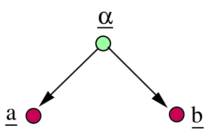
Figure 1: Classical Bayesian Net that motivates the definition of $E_{F}$.

It represents a probability distribution of the form:

$$P(a,b,\alpha)=P(a|\alpha)P(b|\alpha)P(\alpha)\;.$$ (5)

One can easily check that for this probability distribution, $H({\underline{a}}:{\underline{b}}|{\underline{\alpha}})$ is identically zero.

In the classical case, we define $E_{F}$ by

$$E_{F}(P_{{\underline{a}},{\underline{b}}})=\min_{P_{{\underline{a}},{\underline{b}},{\underline{\alpha}}}\in K}H({\underline{a}}:{\underline{b}}|{\underline{\alpha}})\;,$$ (6)

where $K$ is the set of all probability distributions $P_{{\underline{a}},{\underline{b}},{\underline{\alpha}}}$ with a fixed marginal $P_{{\underline{a}},{\underline{b}}}$. Thus, $E_{F}$ is a function of $P_{{\underline{a}},{\underline{b}}}$. If $K$ contains a $P_{{\underline{a}},{\underline{b}},{\underline{\alpha}}}$ of the form given by Eq.(5), then $E_{F}=0$. This is always true if $K$ is defined to contain all probability distributions with arbitrary positive values of $N_{\underline{\alpha}}$. But it may not be true if $K$ contains only probability distributions with a fixed $N_{\underline{\alpha}}$ value. The fact that the right hand side of Eq.(6) vanishes in the classical case (if $K$ includes all $N_{\underline{\alpha}}$ values) is an important motivation for defining $E_{F}$ this way. We want a measure of entanglement that is exclusively quantum.

In the quantum case, suppose $\{w_{\alpha}:\alpha=1,\ldots,N_{\underline{\alpha}}\}$ is a probability distribution for ${\underline{\alpha}}$, and $\{|\alpha\rangle:\alpha=1,\ldots,N_{\underline{\alpha}}\}$ is an orthonormal basis for ${\cal H}_{\underline{\alpha}}$. For all $\alpha$, suppose $\rho^{\alpha}_{\underline{a}}\in{\rm dm}({\cal H}_{\underline{a}})$, and $\rho^{\alpha}_{\underline{b}}\in{\rm dm}({\cal H}_{\underline{b}})$. Consider a “separable” density matrix $\rho_{{\underline{a}},{\underline{b}},{\underline{\alpha}}}$ of the form

$$\rho_{{\underline{a}},{\underline{b}},{\underline{\alpha}}}=\sum_{\alpha}\rho_{\underline{a}}^{\alpha}\rho_{\underline{b}}^{\alpha}w_{\alpha}|\alpha\rangle\langle\alpha|\;.$$ (7)

One can easily check that for this density matrix, $S({\underline{a}}:{\underline{b}}|{\underline{\alpha}})=0$.

In the quantum case, we define $E_{F}$ by

$$E_{F}(\rho_{{\underline{a}},{\underline{b}}})=\min_{\rho_{{\underline{a}},{\underline{b}},{\underline{\alpha}}}\in K}S({\underline{a}}:{\underline{b}}|{\underline{\alpha}})\;,$$ (8)

where $K$ equals the set $K_{0}=\{\rho_{{\underline{a}},{\underline{b}},{\underline{\alpha}}}\in{\rm dm}({\cal H}_{{\underline{a}},{\underline{b}},{\underline{\alpha}}}):$ arbitrary $N_{\underline{\alpha}}$, fixed marginal $\rho_{{\underline{a}},{\underline{b}}}\}$. Thus, $E_{F}$ is a function of $\rho_{{\underline{a}},{\underline{b}}}$. If $K$ contains a $\rho_{{\underline{a}},{\underline{b}},{\underline{\alpha}}}$ of the form given by Eq.(7), then $E_{F}$ is zero. The quantum $E_{F}$ can be nonzero even if $K$ contains all density matrices with arbitrary $N_{\underline{\alpha}}$ values.

In Eq.(8), we could set $K=K_{2}$, where $K_{2}$ is the subset of $K_{0}$ which restricts $\rho_{{\underline{a}},{\underline{b}},{\underline{\alpha}}}$ to be of the form

$$\rho_{{\underline{a}},{\underline{b}},{\underline{\alpha}}}=\sum_{\alpha}|\psi^{\alpha}_{{\underline{a}},{\underline{b}}}\rangle\langle\psi^{\alpha}_{{\underline{a}},{\underline{b}}}|w_{\alpha}|\alpha\rangle\langle\alpha|\;,$$ (9)

where $|\psi^{\alpha}_{{\underline{a}},{\underline{b}}}\rangle\in{\cal H}_{{\underline{a}},{\underline{b}}}$. One can show that Eq.(8) with $K=K_{2}$ is identical (up to a factor of 2) to the definition of $E_{F}$ originally given by Bennett et al in Ref.[1]. Other possible $K$ choices come to mind. For example, one could set $K$ equal to $K_{1}$, where $K_{1}$ is that subset of $K_{0}$ which restricts $\rho_{{\underline{a}},{\underline{b}},{\underline{\alpha}}}$ to be of the form

$$\rho_{{\underline{a}},{\underline{b}},{\underline{\alpha}}}=\sum_{\alpha}\rho^{\alpha}_{{\underline{a}},{\underline{b}}}w_{\alpha}|\alpha\rangle\langle\alpha|\;,$$ (10)

where $\rho^{\alpha}_{{\underline{a}},{\underline{b}}}\in{\rm dm}({\cal H}_{{\underline{a}},{\underline{b}}})$ need not be pure. $K_{0},K_{1},K_{2}$ represent different degrees of information about how $\rho_{{\underline{a}},{\underline{b}},{\underline{\alpha}}}$ was created. $K_{0}$ represents total ignorance.

3 Classical Distillation

In this section, we will define a classical $E_{D}$. In the next section, we will find a quantum counterpart for it.

Consider the Classical Bayesian Net of Fig.2.

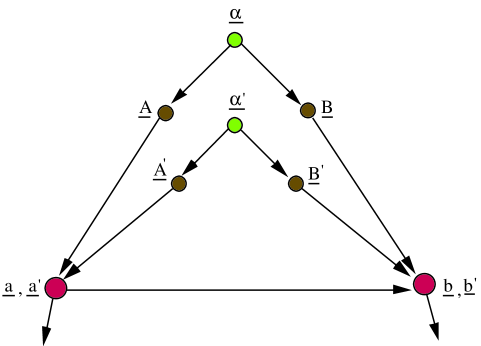
Figure 2: Classical Bayesian Net that motivates the definition of $E_{D}$.

The arrow from $({\underline{a}},{\underline{a}}^{\prime})$ to $({\underline{b}},{\underline{b}}^{\prime})$ allows what is often referred to as “classical communication from Alice to Bob”. Let ${\underline{X}}=({\underline{A}},{\underline{B}})$, ${\underline{X}}^{\prime}=({\underline{A}}^{\prime},{\underline{B}}^{\prime})$. Let $N_{\underline{A}}=N_{{\underline{A}}^{\prime}}=N_{\underline{a}}=N_{{\underline{a}}^{\prime}}$ and $N_{\underline{B}}=N_{{\underline{B}}^{\prime}}=N_{\underline{b}}=N_{{\underline{b}}^{\prime}}$. The net of Fig.2 satisfies:

$$P(a,b,a^{\prime},b^{\prime})=\sum_{X,X^{\prime}}P(a,a^{\prime}|A,A^{\prime})P(b,b^{\prime}|B,B^{\prime},a,a^{\prime})P(X)P(X^{\prime})\;,$$ (11)

where

$$P(X)=\sum_{\alpha}P(A|\alpha)P(B|\alpha)P(\alpha)\;,$$ (12a)

and

$$P(X^{\prime})=\sum_{\alpha^{\prime}}P(A^{\prime}|{\alpha^{\prime}})P(B^{\prime}|{\alpha^{\prime}})P({\alpha^{\prime}})\;.$$ (12b)

We wish to consider only those experiment in which ${\underline{a}}^{\prime}$ and ${\underline{b}}^{\prime}$ are both fixed at a known value, call it 0 for definiteness. For such experiments, one considers:

$$P(a,b|a^{\prime}=b^{\prime}=0)=\frac{P(a,b,a^{\prime}=0,b^{\prime}=0)}{P(a^{\prime}=0,b^{\prime}=0)}\;.$$ (13)

Henceforth we will use $\Gamma$ as a short-hand for the string “${\underline{a}}^{\prime}=0,{\underline{b}}^{\prime}=0$”. We will also use $U$ to denote $P_{{\underline{a}},{\underline{a}}^{\prime}|{\underline{A}},{\underline{A}}^{\prime}}$ and $V$ to denote $P_{{\underline{b}},{\underline{b}}^{\prime}|{\underline{B}},{\underline{B}}^{\prime},{\underline{a}},{\underline{a}}^{\prime}}$.

In the classical case, we define $E_{D}$ by

$$E_{D}(P_{\underline{X}},P_{{\underline{X}}^{\prime}})=\max_{U,V}\min_{P_{{\underline{a}},{\underline{b}},{\underline{\lambda}}|\Gamma}\in K}H({\underline{a}}:{\underline{b}}|{\underline{\lambda}},\Gamma)\;,$$ (14)

where $K$ is the set of all probability distributions $P_{{\underline{a}},{\underline{b}},{\underline{\lambda}}|\Gamma}$ with a fixed marginal $P_{{\underline{a}},{\underline{b}}|\Gamma}$ that satisfies Eq.(11). $P_{{\underline{a}},{\underline{b}}|\Gamma}$ depends on $P_{\underline{X}},P_{{\underline{X}}^{\prime}},U,V$. Since we maximize over $U,V$, $E_{D}$ is a function of $P_{\underline{X}}$ and $P_{{\underline{X}}^{\prime}}$.

Next we will show that the net of Fig.2, without the classical communication arrow, satisfies:

$$E_{D}(P_{\underline{X}},P_{{\underline{X}}^{\prime}})\leq E_{F}(P_{\underline{X}})+E_{F}(P_{{\underline{X}}^{\prime}})\;.$$ (15)

Suppose we could show that

$$H({\underline{a}}:{\underline{b}}|{\underline{\alpha}},{\underline{\alpha}}^{\prime},\Gamma)\leq H(({\underline{A}},{\underline{A}}^{\prime}):({\underline{B}},{\underline{B}}^{\prime})|{\underline{\alpha}},{\underline{\alpha}}^{\prime})\;.$$ (16)

After taking limits on the left hand side, this gives

$$E_{D}\leq H({\underline{A}},{\underline{A}}^{\prime}:{\underline{B}},{\underline{B}}^{\prime}|{\underline{\alpha}},{\underline{\alpha}}^{\prime})\;.$$ (17)

Note that by the independence of the prime and unprimed variables

$$H({\underline{A}},{\underline{A}}^{\prime}:{\underline{B}},{\underline{B}}^{\prime}|{\underline{\alpha}},{\underline{\alpha}}^{\prime})=H({\underline{A}}:{\underline{B}}|{\underline{\alpha}})+H({\underline{A}}^{\prime}:{\underline{B}}^{\prime}|{\underline{\alpha}}^{\prime})\;.$$ (18)

Eqs.(17) and (18) imply Eq.(15). So let us concentrate on establishing Eq.(16). Events ${\underline{A}},{\underline{A}}^{\prime},{\underline{B}},{\underline{B}}^{\prime}$ all occur before $\Gamma$ so they are independent of $\Gamma$. Therefore, we can write:

$$H({\underline{A}},{\underline{A}}^{\prime}:{\underline{B}},{\underline{B}}^{\prime}|{\underline{\alpha}},{\underline{\alpha}}^{\prime})=H({\underline{A}},{\underline{A}}^{\prime}:{\underline{B}},{\underline{B}}^{\prime}|{\underline{\alpha}},{\underline{\alpha}}^{\prime},\Gamma)\;.$$ (19)

Because of Eq.(19), Eqs.(16) is equivalent to:

$$H({\underline{a}}:{\underline{b}}|{\underline{\alpha}},{\underline{\alpha}}^{\prime},\Gamma)\leq H({\underline{A}},{\underline{A}}^{\prime}:{\underline{B}},{\underline{B}}^{\prime}|{\underline{\alpha}},{\underline{\alpha}}^{\prime},\Gamma)\;.$$ (20)

Eq.(20) follows easily from the following Lemma, which is proven in AppendixA. Lemma: The net of Fig.3 satisfies

$$H({\underline{a}}:{\underline{b}}|{\underline{\lambda}})\leq H({\underline{x}}:{\underline{y}}|{\underline{\lambda}})\;.$$ (21)

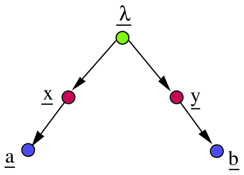
Figure 3: Classical Bayesian Net that obeys the Data Processing Inequality Eq.(21).

4 Quantum Distillation

In this section, we will give a quantum counterpart of the classical $E_{D}$ defined in the previous section.

As in the classical case, let ${\underline{X}}=({\underline{A}},{\underline{B}})$, ${\underline{X}}^{\prime}=({\underline{A}}^{\prime},{\underline{B}}^{\prime})$. Let $N_{\underline{A}}=N_{{\underline{A}}^{\prime}}=N_{\underline{a}}=N_{{\underline{a}}^{\prime}}$ and $N_{\underline{B}}=N_{{\underline{B}}^{\prime}}=N_{\underline{b}}=N_{{\underline{b}}^{\prime}}$. Suppose $\rho_{\underline{X}}\in{\rm dm}({\cal H}_{\underline{X}})$ and $\rho_{{\underline{X}}^{\prime}}\in{\rm dm}({\cal H}_{{\underline{X}}^{\prime}})$ are given. Suppose $U_{{\underline{a}},{\underline{a}}^{\prime}|{\underline{A}},{\underline{A}}^{\prime}}$ is a unitary transformation mapping ${\cal H}_{{\underline{A}},{\underline{A}}^{\prime}}$ onto ${\cal H}_{{\underline{a}},{\underline{a}}^{\prime}}$:

$$U^{\dagger}_{{\underline{A}},{\underline{A}}^{\prime}|{\underline{a}},{\underline{a}}^{\prime}}U_{{\underline{a}},{\underline{a}}^{\prime}|{\underline{A}},{\underline{A}}^{\prime}}=1\;.$$ (22)

Likewise, suppose that for each $a$, $V^{a}_{{\underline{b}},{\underline{b}}^{\prime}|{\underline{B}},{\underline{B}}^{\prime}}$is a unitary transformation mapping ${\cal H}_{{\underline{B}},{\underline{B}}^{\prime}}$ onto ${\cal H}_{{\underline{b}},{\underline{b}}^{\prime}}$:

$$V^{\dagger a}_{{\underline{B}},{\underline{B}}^{\prime}|{\underline{b}},{\underline{b}}^{\prime}}V_{{\underline{b}},{\underline{b}}^{\prime}|{\underline{B}},{\underline{B}}^{\prime}}^{a}=1\;.$$ (23)

Define the following projector on ${\cal H}_{\underline{a}}$:

$$\pi_{\underline{a}}^{a}=|a\rangle_{\underline{a}}\langle a|_{\underline{a}}\;.$$ (24)

Now consider the following density matrix

$$\rho_{{\underline{a}},{\underline{b}}|\Gamma}=\frac{1}{P(\Gamma)}\sum_{a}\langle 0_{{\underline{a}}^{\prime}},0_{{\underline{b}}^{\prime}}|\pi_{\underline{a}}^{a}U_{{\underline{a}},{\underline{a}}^{\prime}|{\underline{A}},{\underline{A}}^{\prime}}V_{{\underline{b}},{\underline{b}}^{\prime}|{\underline{B}},{\underline{B}}^{\prime}}^{a}\rho_{\underline{X}}\rho_{{\underline{X}}^{\prime}}V^{\dagger a}_{{\underline{B}},{\underline{B}}^{\prime}|{\underline{b}},{\underline{b}}^{\prime}}U^{\dagger}_{{\underline{A}},{\underline{A}}^{\prime}|{\underline{a}},{\underline{a}}^{\prime}}\pi_{\underline{a}}^{a}|0_{{\underline{a}}},0_{{\underline{b}}^{\prime}}\rangle\;,$$ (25)

where $P(\Gamma)$ is defined so that ${\rm tr}_{{\underline{a}},{\underline{b}}}(\rho_{{\underline{a}},{\underline{b}}|\Gamma})=1$. The previous equation can also be expressed in index notation as:

$$\langle a,b_{1}|\rho_{{\underline{a}},{\underline{b}}|\Gamma}|a,b_{2}\rangle = \frac{1}{P(\Gamma)}\langle a,a^{\prime}=0|U_{{\underline{a}},{\underline{a}}^{\prime}|{\underline{A}},{\underline{A}}^{\prime}}|{\color[rgb]{1,0,0}{A_{1}}},{\color[rgb]{1,0,0}{A^{\prime}_{1}}}\rangle$$ (31)

$$\langle b_{1},b^{\prime}=0|V^{a}_{{\underline{b}},{\underline{b}}^{\prime}|{\underline{B}},{\underline{B}}^{\prime}}|{\color[rgb]{1,0,0}{B_{1}}},{\color[rgb]{1,0,0}{B^{\prime}_{1}}}\rangle$$

$$\langle{\color[rgb]{1,0,0}{A_{1}}},{\color[rgb]{1,0,0}{B_{1}}}|\rho_{\underline{X}}|{\color[rgb]{1,0,0}{A_{2}}},{\color[rgb]{1,0,0}{B_{2}}}\rangle$$

$$\langle{\color[rgb]{1,0,0}{A_{1}^{\prime}}},{\color[rgb]{1,0,0}{B^{\prime}_{1}}}|\rho_{{\underline{X}}^{\prime}}|{\color[rgb]{1,0,0}{A^{\prime}_{2}}},{\color[rgb]{1,0,0}{B^{\prime}_{2}}}\rangle$$

$$\langle{\color[rgb]{1,0,0}{B_{2}}},{\color[rgb]{1,0,0}{B^{\prime}_{2}}}|V^{\dagger a}_{{\underline{B}},{\underline{B}}^{\prime}|{\underline{b}},{\underline{b}}^{\prime}}|b_{2},b^{\prime}=0\rangle$$

$$\langle{\color[rgb]{1,0,0}{A_{2}}},{\color[rgb]{1,0,0}{A^{\prime}_{2}}}|U^{\dagger}_{{\underline{A}},{\underline{A}}^{\prime}|{\underline{a}},{\underline{a}}^{\prime}}|a,a^{\prime}=0\rangle\;.$$

Finally, we define $E_{D}$ by

$$E_{D}(\rho_{\underline{X}},\rho_{{\underline{X}}^{\prime}})=\max_{U,V}\min_{\rho_{{\underline{a}},{\underline{b}},{\underline{\lambda}}|\Gamma}\in K}S({\underline{a}}:{\underline{b}}|{\underline{\lambda}},\Gamma)\;,$$ (32)

where $K$ contains all density matrices $\rho_{{\underline{a}},{\underline{b}},{\underline{\lambda}}|\Gamma}$ with a fixed marginal $\rho_{{\underline{a}},{\underline{b}}|\Gamma}$ that satisfies Eq.(25).

Appendix A Appendix: Some Data Processing Inequalities

In this appendix, we will prove two well known Data Processing Inequalities.

If $P,Q\in{\rm pd}(S_{\underline{x}})$, then the relative entropy (or Kullback-Leibler distance) between $P$ and $Q$ is

$$D(P//Q)=\sum_{x}P(x)\ln[P(x)/Q(x)]\;.$$ (33)

Lemma A.1

(Data Processing Inequality for Relative Entropy, see Ref.[8]) If $P,Q\in{\rm pd}(S_{\underline{x}})$ and $T=\{T(y|x):y\in S_{\underline{y}},x\in S_{\underline{x}}\}$ is a matrix of non-negative numbers such that $\sum_{y}T(y|x)=1$, then

$$D(P//Q)\geq D(TP//TQ)\;,$$ (34)

where $TP$ should be understood as the matrix product of the column vector $P$ times the matrix $T$.

proof:

One has

$$D(P//Q) = \sum_{x}P(x)\ln\left(\frac{P(x)}{Q(x)}\right)$$ (35)

$$= \sum_{y}\sum_{x}T(y|x)P(x)\ln\left(\frac{T(y|x)P(x)}{T(y|x)Q(x)}\right)$$ (36)

$$\geq \sum_{y}TP(y)\ln\left(\frac{TP(y)}{TQ(y)}\right)=D(TP//TQ)\;.$$ (37)

Line (37) follows from an application of the Log-Sum Inequality[9]. QED

Lemma A.2

(Data Processing Inequality for CMI) The net of Fig.3 satisfies

$$H({\underline{x}}:{\underline{y}}|{\underline{\lambda}})\geq H({\underline{a}}:{\underline{b}}|{\underline{\lambda}})\;.$$ (38)

proof:

The net of Fig.3 represent a probability distribution of the form:

$$P(a,b,x,y,\lambda)=P(a|x)P(b|y)P(x|\lambda)P(y|\lambda)P(\lambda)\;.$$ (39)

One can easily show that such a probability distribution satisfies:

$$P(a|\lambda)=\sum_{x}P(a|x)P(x|\lambda)\;,$$ (40a)

$$P(b|\lambda)=\sum_{y}P(b|y)P(y|\lambda)\;,$$ (40b)

$$P(a,b|\lambda)=P(a|\lambda)P(b|\lambda)\;,$$ (41a)

$$P(x,y|\lambda)=P(x|\lambda)P(y|\lambda)\;.$$ (41b)

For any two random variables ${\underline{\lambda}},{\underline{x}}$, let $Q^{\lambda}_{\underline{x}}$ be shorthand for $P_{{\underline{x}}|{\underline{\lambda}}=\lambda}$. In other words, $Q^{\lambda}_{\underline{x}}(x)=P_{{\underline{x}}|{\underline{\lambda}}}(x|\lambda)$ for all $x,\lambda$. The two CMI we are dealing with can be rewritten in terms of relative entropy as follows:

$$H({\underline{x}}:{\underline{y}}|{\underline{\lambda}})=\sum_{\lambda}P(\lambda)D(Q^{\lambda}_{{\underline{x}},{\underline{y}}}//Q^{\lambda}_{{\underline{x}}}Q^{\lambda}_{{\underline{y}}})\;,$$ (42)

and

$$H({\underline{a}}:{\underline{b}}|{\underline{\lambda}})=\sum_{\lambda}P(\lambda)D(Q^{\lambda}_{{\underline{a}},{\underline{b}}}//Q^{\lambda}_{{\underline{a}}}Q^{\lambda}_{{\underline{b}}})\;.$$ (43)

Thus, if we can show that

$$D(Q^{\lambda}_{{\underline{x}},{\underline{y}}}//Q^{\lambda}_{{\underline{x}}}Q^{\lambda}_{{\underline{y}}})\geq D(Q^{\lambda}_{{\underline{a}},{\underline{b}}}//Q^{\lambda}_{{\underline{a}}}Q^{\lambda}_{{\underline{b}}})\;,$$ (44)

then the present Lemma will be proven. The last inequality will follow from Lemma A.1 if we can find a transition probability matrix $T(a,b|x,y)$ such that

$$P(a,b|\lambda)=\sum_{x,y}T(a,b|x,y)P(x,y|\lambda)\;,$$ (45a)

and

$$P(a|\lambda)P(b|\lambda)=\sum_{x,y}T(a,b|x,y)P(x|\lambda)P(y|\lambda)\;.$$ (45b)

Eqs.(45b) follow easily from Eqs.(40b) and (41b), with $T$ given by :

$$T(a,b|x,y)=P(a|x)P(b|y)\;.$$ (46)

QED

References

• [1] C.H. Bennett, D.P. DiVincenzo, J.A. Smolin, W.K. Wootters, “Mixed State Entanglement and Quantum Error Correction”, quant-ph/9604024 .
• [2]
• R.R. Tucci, “Quantum Entanglement and Conditional Information Transmission”, quant-ph/9909041
• R.R. Tucci, “Separability of Density Matrices and Conditional Information Transmission”, quant-ph/0005119
• R.R. Tucci, “Entanglement of Formation and Conditional Information Transmission”, quant-ph/0010041
• R.R. Tucci, “Relaxation Method For Calculating Quantum Entanglement”, quant-ph/0101123
• R.R. Tucci, “Entanglement of Bell Mixtures of Two Qubits”, quant-ph/0103040
• [3] B.M. Terhal, M. Horodecki, D.W. Leung, D.P. DiVincenzo, “The entanglement of purification”, quant-ph/0202044 .
• [4] R.R. Tucci, “Quantum Information Theory - A Quantum Bayesian Net Perspective”, quant-ph/9909039 .
• [5] Elements of Information Theory, by T.M. Cover and J.A. Thomas, (Wiley 1991).
• [6] W.J. McGill, “Multivariate Information Transmission”, IRE Trans. Info. Theory 4(1954) 93-111.
• [7] Ref.[5], page 44, exercise 10.
• [8] This Data Processing Inequality for Relative Entropy is well known. Ref.[5] mentions it on page 300. Our proof of the inequality comes from page 55 of the book by I. Csiszar and J. Korner, “Information Theory-Coding Theorems for Discrete Memoryless Systems”, (Academic Press, 1981).
• [9] Log-Sum Inequality is discussed in Ref.[5], page 29.