Changes of the topological charge of vortices

Abstract

We consider changes of the topological charge of vortices in quantum mechanics by investigating analytical examples where the creation or annihilation of vortices occurs. In classical hydrodynamics of non-viscous fluids the Helmholtz-Kelvin theorem ensures that the velocity field circulation is conserved. We discuss applicability of the theorem in the hydrodynamical formulation of quantum mechanics showing that the assumptions of the theorem may be broken in quantum evolution of the wavefunction leading to a change of the topological charge.

I Introduction

Vortices can be found both in classical and quantum physics. One can encounter vortices, for instance, in water that spins around or in the air as a ring of smoke [1]. Quantum mechanics can be formulated in a language of hydrodynamics (see e.g. [2, 3] and references therein). Such a formulation (very useful also in quantum chemistry [2]) provides a basis for definition of topological defects like vortices  [4], whose features are even more striking than those that we find in classical physics. Quantum vortices appear not only in systems described by the linear Schrödinger equation. Indeed, they were experimentally observed in superfluid HeII [5] and a Bose-Einstein condensate (BEC) of trapped alkali atoms  [6, 7] which are typically described, within the mean-field approximation, by a nonlinear equation [8].

In hydrodynamics of ordinary non-viscous fluids, the circulation of the velocity field is conserved in time evolution due to the celebrated Helmholtz-Kelvin theorem (HKT) [9]. This theorem is often employed in quantum mechanics [3, 4, 10, 11]. However, uncritical usage of the HKT, may lead to the incorrect conclusion that stability of vortices and vortex rings in quantum fluids is fully guaranteed by the HKT [11]. In the present paper we discuss the basic assumptions of the HKT and show analytical examples where these assumptions can be easily broken by quantum evolution of the wave function, leading to changes of the topological charge. Difficulties in fulfilling the assumptions of the HKT have been already pointed out in conclusions of Ref. [12].

II Hydrodynamical formulation of quantum mechanics

To establish connections between quantum mechanics and fluid dynamics we write the wave function in the form $\Psi(\vec{r},t)=\sqrt{\rho(\vec{r},t)}\exp(i\chi(\vec{r},t))$ [2], (where $\rho(\vec{r},t)$ stands for density of a probability fluid) and define the velocity field

$$\vec{v}=\frac{\hbar}{m}\vec{\nabla}\chi(\vec{r},t).$$ (1)

Provided $\vec{v}$ and its partial derivatives are well defined, we may rewrite the Schrödinger equation [with a potential $V(\vec{r},t)$] in the form

$$m\frac{\partial\vec{v}}{\partial t}+\vec{\nabla}\left(\frac{1}{2}mv^{2}+V-\frac{\hbar^{2}}{2m}\frac{\nabla^{2}\sqrt{\rho}}{\sqrt{\rho}}\right)=0,$$ (2)

$$\frac{\partial\rho}{\partial t}+\vec{\nabla}\cdot\left(\vec{v}\rho\right)=0.$$ (3)

Equation (3) is an ordinary continuity equation, while Eq. (2), in the limit of $\hbar\rightarrow 0$, becomes similar to the dynamical equation of a curl-free non-viscous fluid [9].

In quantum mechanics the wave function has to be single valued. To satisfy this condition one arrives at the Feynman-Onsager quantization condition [13] for the circulation of the velocity field $\Gamma_{C}$ around any closed contour $C$

$$\Gamma_{C}=\oint_{C}\vec{v}\cdot d\vec{l}=n\frac{2\pi\hbar}{m},$$ (4)

where $n=0,\pm 1,\pm 2,\dots$. Due to the definition (1), we may not expect $n\neq 0$ unless at a certain point on a surface encircled by the contour $C$, $\vec{\nabla}\times\vec{v}$ becomes singular (behaves as a Dirac delta function, see for example [5]). We refer to $n$ as a topological charge since any continuous deformation of the contour $C$, which does not incorporate any other points where curl of the velocity field does not vanish, can not change $\Gamma_{C}$.

III The Helmholtz-Kelvin theorem

One may ask whether the circulation $\Gamma_{C}$ is conserved in time evolution of the velocity field. For a fixed contour, a possibly moving vortex may leave an area bounded by the contour and consequently $\Gamma_{C}$ changes its value. Thus, the relevant situation we should consider corresponds to the case where we let an initially defined contour evolve in time according to the velocity field.

Parameterizing the initial contour by $\xi$ variable, i.e. $C(t_{0})=\{\vec{r}(\xi,t_{0})\}$, and employing the equation of motion of a contour

$$\frac{d}{dt}\vec{r}(\xi,t)=\vec{v}[\vec{r}(\xi,t)],$$ (5)

yields

$$\frac{d}{dt}\Gamma_{C(t)}=\oint_{C(t)}\left(\frac{\partial\vec{v}}{\partial t}+(\vec{v}\cdot\vec{\nabla})\vec{v}+\frac{1}{2}\vec{\nabla}v^{2}\right)\cdot d\vec{l}.$$ (6)

If the contour is drawn through points where the velocity field $\vec{v}$ and its partial derivatives are well defined, applying: Eq. (2), equality $(\vec{v}\cdot\vec{\nabla})\vec{v}=\frac{1}{2}\vec{\nabla}v^{2}-\vec{v}\times(\vec{\nabla}\times\vec{v})$, and using the fact that, at least on the contour $\vec{\nabla}\times\vec{v}=0$, we get

$$\frac{d}{dt}\Gamma_{C(t)}=0.$$ (7)

Equation (7) establishes the Helmholtz-Kelvin theorem originally proved for a non-viscous fluid [9]. Applicability of this theorem to a non-linear quantum systems is presented in the Appendix.

The HKT is fulfilled provided the contour $C(t)$ that goes initially through points where the velocity field is well defined will evolve in time through such points only. In the following we will see how such an assumption may be broken by quantum evolution of the wave function leading to a change of the topological charge.

IV Analytical examples

In this section we discuss a few possibilities of breaking of the HKT. To this end we analyze three different analytically solvable examples where breaking of the HKT becomes evident.

First example shows that changes of the topological charge of a vortex correspond to the appearance of a nodal line of the wave function. In Ref. [14] the authors show the instability of a vortex placed in an anisotropic two-dimensional harmonic trap. We would like to discuss the source of violation of the HKT in such a case. We will calculate the velocity field and analyze changes of its circulation from a point of view of the HKT.

Consider an anisotropic two-dimensional harmonic oscillator with the potential

$$V(x,y)=\frac{1}{2}x^{2}+\frac{\lambda^{2}}{2}y^{2},$$ (8)

(where we use the units of the harmonic oscillator corresponding to the $x$-direction). The initial wave function is prepared as a superposition of the two lowest excited states

$$\Psi(x,y)\propto(x+i\alpha y)e^{-(x^{2}+\lambda y^{2})/2},$$ (9)

with a real parameter $\alpha>0$. Choosing any contour $C$ that encircles the origin of the coordinate frame we find out that the circulation $\Gamma_{C}$ corresponds to $n=1$ vortex. However, the circulation around that point is not conserved in time. Indeed, analysis of time evolution of the velocity field

$$\vec{v}(x,y,t)=\frac{\alpha\ \cos(Et)}{x^{2}+y^{2}\ \alpha^{2}+2\alpha xy\sin(Et)}(-y\vec{e}_{x}+x\vec{e}_{y}),$$ (10)

(where $E=\lambda-1$ is the energy difference of the two lowest excited states) reveals that for $Et\in[0,\pi/2)$, $\Gamma_{C}$ corresponds to $n=1$ while for $Et\in(\pi/2,\pi]$ to $n=-1$.

To discuss applicability of the HKT we have to investigate time evolution of the initially defined contour. The problem requires careful treatment because for $Et=\pi/2-\varepsilon$ (where $\varepsilon\rightarrow 0^{+}$) the velocity field goes to zero everywhere except on the nodal line, $x+\alpha y=0$, where it diverges $\vec{v}\rightarrow\frac{1}{\varepsilon x}(\vec{e}_{x}+\alpha\vec{e}_{y})$. To demonstrate violation of the HKT we have to show that a contour initially encircling the center is not extended to infinity but indeed faces singularity for $Et=\pi/2$.

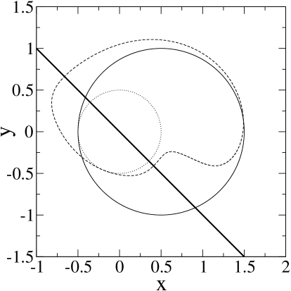
FIG. 1.: Plot of the contour encircling the center of the trap for $Et\rightarrow\pi/2$ (dashed line). The contour was initially ($t=0$) chosen to be a circle with the unit radius centered at $(0.5,0)$ (solid line). The thick solid line represents the nodal line given by the equation $x+\alpha y=0$. Initially, the point of the contour closest to the origin of the coordinates is situated at the distance $0.5$. Therefore in course of the evolution none of the points of the contour can get closer to the origin than at the distance 0.5, i.e. can not cross the dotted circle with the radius $0.5$ that is centered at $(0,0)$. For this presentation we have chosen $\lambda=\sqrt{2}$, $\alpha=1$ — see text for details.

Suppose we define a contour, encircling the origin, at a time $t=0$, and look for a time evolution of its arbitrary point $i$, whose position we denote by $\{x_{i}(t),y_{i}(t)\}$. Combining Eq. (5) and Eq. (10) we get

$$\frac{dx_{i}}{dt}=-f(x_{i},y_{i})\;y_{i},\ \ \ \frac{dy_{i}}{dt}=f(x_{i},y_{i})\;x_{i},$$ (11)

with

$$f(x,y)=\frac{\alpha\cos(Et)}{x^{2}+y^{2}\ \alpha^{2}+2\alpha xy\sin(Et)}.$$ (12)

From Eq. (11) it is apparent that the distance of the point $\{x_{i}(t),y_{i}(t)\}$ from the origin does not change in course of the evolution. Indeed the quantity $x_{i}(t)^{2}+y_{i}(t)^{2}$ is a constant of motion as long as the function (12) is well defined. Note that it diverges, at $Et=\pi/2$, for points lying on the nodal line. Therefore, for $Et=\pi/2-\varepsilon$ with arbitrary small $\varepsilon>0$ nothing extraordinary happens with the contour until at $Et=\pi/2$ the contour faces singularity (see Fig. 1 for an example of the contour evolution). Thus, the HKT can not be applied because quantum evolution of the wave function pushes an evolving contour to singular points and the quantities involved in the theorem become undefined.

We would like to stress that the presented scenario where the vortex situated in the harmonic trap reveals periodic changes of the topological charge is possible only when the initial vortex is placed exactly at the center of the potential. Otherwise the vortex changes its position — it escapes to infinity and another vortex with the opposite charge arrives from infinity and the scenario repeats periodically.

In the second example we would like to present violation of the HKT due to annihilation of a vortex ring. This example comes from Ref. [4] where creation and annihilation of a vortex ring for freely moving particle is presented. Even though it is not clearly stated in Ref. [4], the HKT is not fulfilled in that case. The wave function of a vortex ring [4] (in dimensionless units) may be written in the form

$$\Psi(x,y,z,t) \propto [(x-kt)^{2}+y^{2}+z^{2}-1$$ (13)

$$+ i3(z+t)]e^{ikx-ik^{2}t/2},$$ (14)

where the wave vector $\vec{k}=(k,0,0)$ is related to a motion of the “center of mass” of the vortex ring with a constant velocity $\vec{k}$. The vortex ring corresponds to the nodal line of the wave function and is located at the intersection of the plane $z+t=0$ and sphere $(x-kt)^{2}+y^{2}+z^{2}=1$. At time $t=-1$, the vortex is born at a point $(-k,0,1)$ and, at time $t=1$, it disappears at a point $(k,0,-1)$. The radius of the vortex changes in time as $\sqrt{1-t^{2}}$.

Suppose at any time $t\in(-1,1)$, we define a contour $C$ so that it encircles the vortex (see Fig. 2) and the circulation of the velocity field corresponds to $n=1$. The evolving contour can not cross the vortex ring without facing a singularity in the velocity field. However, the ring at some moment starts shrinking and at $t=1$ it reduces to a point. Consequently, at $t=1$, the contour must go through a singularity of the velocity field and the integral (6) and also the HKT become meaningless.

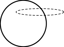
FIG. 2.: Schematic plot of the nodal line corresponding to a vortex ring (solid line) and a contour that encircles the ring (dashed line). In last stage of time evolution the ring shrinks to a point and the contour faces singularity.

The last example we would like to comment on shows collision of two vortices leading to the appearance of a single doubly charged vortex. Consider, for simplicity, a two-dimensional H atom initially in the first excited state with angular momentum $L_{z}=1$ [i.e. $\psi_{1}(r,\varphi)\propto r\exp(-2r/3)\exp(i\varphi)$ in atomic units] that is driven resonantly by a circularly polarized electromagnetic field. The field frequency is tuned to the transition between the first and second excited energy eigenstates. It results in the familiar Rabi oscillation [15] between the $\psi_{1}(r,\varphi)$ state and the second excited state with angular momentum $L_{z}=2$ [i.e. $\psi_{2}(r,\varphi)\propto r^{2}\exp(-2r/5)\exp(i2\varphi)$]. Indeed, the time evolution of the wavefunction reads

$$|\psi(t)\rangle\propto\cos(Dt)e^{-iE_{1}t}\;|\psi_{1}\rangle+e^{-iE_{2}t}\sin(Dt)\;|\psi_{2}\rangle\ ,$$ (15)

where $D$ is a dipole matrix element [15]; $E_{1}$, $E_{2}$ are energies of $|\psi_{1}\rangle$, $|\psi_{2}\rangle$ states.

For $t=0$ there is a vortex with $n=1$ at the center of the coordinates as expected for the state with angular momentum $L_{z}=1$. When $Dt$ increases another vortex with $n=1$ moves in from infinity, collides with the first one (situated at the center of the coordinates during the whole time evolution) at $Dt=\pi/2$ and then moves out to infinity again and so on. During the collision, i.e. for $Dt=\pi/2$, a single vortex with $n=2$ is formed. In the considered example, the HKT does not apply: if we define a contour so that it encircles the vortex with $n=1$ situated at the center of the coordinate, such a contour encounters a singularity in the velocity field during the collision with the other vortex. Such a behavior, is expected to hold in an arbitrary collision between two vortices leading to formation of one, doubly charged, vortex.

These examples are not the only ones illustrating that vortices can disappear or change their charge in the course of time evolution. They were chosen to illustrate that such processes can happen in different physical systems and results in the violation of the HKT. The theorem is explored in the context of vortices’ stability (see e.g.  [11]) to imply the constancy of a vortex topological charge. As we have clearly illustrated the HKT can not assure persistence of vortex currents in the quantum mechanical systems. Therefore we conclude that the vortex topological charge is not as robust quantity as it is commonly believed (see e. g. [14] and references therein, [16]). Finally, we would like to mention that appearance of vortices can happen in a way that does not violate the HKT. Namely, they can appear in the form of a closed vortex line that springs from a point or as a vortex-antivortex pair creation from a node of a wave function [4].

V Summary and conclusions

We have analyzed the applicability of the Helmholtz-Kelvin theorem in the hydrodynamical formulation of the quantum mechanics. The velocity field of the probability fluid is defined as the gradient of the phase of the quantum wave function. This implies that nonzero circulation, along a given contour, may come out in the system if the field reveals a singularity at certain points on a surface encircled by the contour. Adopting the HKT to the quantum liquid may suggest that such a topological charge of the system can not change.

However, the HKT may be employed if a given contour evolves through points where the velocity field is well defined. It may happen even in classical hydrodynamics that such an assumption is not fulfilled if, e.g., liquid encounters obstacles in the flow [9]. In quantum liquids the situation is more complicated because a singularity is necessary for a nonzero circulation. Indeed, phase of a wave function is undefined at a vortex core, which means that singularities appear in hydrodynamical formulation of quantum mechanics whenever vortices show up. This property makes distinction of hydrodynamical description of quantum system from the classical hydrodynamics. We have presented simple analytical examples where the quantum evolution of a wave function pushes a contour to a singular point. Such a process is accompanied by a change of the vortex topological charge.

We have illustrated the violation of the HKT choosing examples that correspond to linear quantum systems. Macroscopic quantum behavior is present in interacting many particle systems that are usually described in the mean field approximation by a nonlinear Schrödinger equation. In Appendix we complete the analysis of the HKT for a nonlinear Schrödinger evolution. Vortices maybe also investigated in propagation of classical light [16, 17]. Indeed, the evolution equation of the slowly varying envelope of a light beam can have identical form as the Schrödinger equation, which allows for exactly the same considerations as we have presented above. The dynamics of vortices and escapes of the off-center vortex in an analog of the asymmetric harmonic potential have been experimentally observed in such systems [18].

We are grateful to J. Zakrzewski and G. Molina-Terriza for fruitful discussion and to U. Fischer for the critical reading of the manuscript. Support of KBN under project 5 P03B 088 21 is acknowledged.

VI Appendix: Helmholtz-Kelvin theorem for nonlinear systems

For completeness we analyze here the application of the HKT in hydrodynamical formulation of nonlinear quantum mechanics. The so-called Gross-Pitaevskii equation is successfully used to describe the properties of a Bose-Einstein condensate in trapped alkali atoms [8]. In particular this equation exhibits various vortex solutions [11]. To make the discussion more general we will also include the mean field term describing a possible dipolar interactions between condensed atoms [19]. The nonlinear Schrödinger equation of interest reads

$$i\hbar\frac{\partial}{\partial t}\Psi(\vec{r},t)= - \frac{\hbar^{2}}{2m}\vec{\nabla}^{2}\Psi(\vec{r},t)+V(\vec{r},t)\Psi(\vec{r},t)$$ (16)

$$+ \left(\int d^{3}r^{\prime}V_{int}(\vec{r}-\vec{r}^{\prime})|\Psi(\vec{r}^{\prime},t)|^{2}\right)\Psi(\vec{r},t),$$ (17)

where $V_{int}$ corresponds to two body interactions (e.g. point or dipolar interactions [8, 19]). Substitution $\Psi(\vec{r},t)=\sqrt{\rho(\vec{r},t)}\exp(i\chi(\vec{r},t))$ leads to the continuity equation (3) and the following dynamical equation for the velocity field

$$m\frac{\partial\vec{v}}{\partial t} + \vec{\nabla}\left(\frac{1}{2}mv^{2}+V+\int d^{3}r^{\prime}V_{int}(\vec{r}-\vec{r}^{\prime})\rho(\vec{r}^{\prime},t)\right.$$ (18)

$$- \left.\frac{\hbar^{2}}{2m}\frac{\nabla^{2}\sqrt{\rho}}{\sqrt{\rho}}\right)=0.$$ (19)

The only difference in comparison with Eq. (2) is the appearance of two new terms in the bracket of Eq. (18). These terms, however, do not change the proof of the HKT — for example Eq. (6) does not possess any potential like terms. Therefore the Helmholtz-Kelvin theorem holds also for systems described by Eq. (16) under the same assumptions as in the case of linear quantum mechanics discussed in Sec. III.

REFERENCES

- [1] R. P. Feynman, R. B. Leighton, M. Sands, The Feynman Lectures on Physics, Volume II, (Addison-Wesley Publishing Company, Massachusetts, 1963).
- [2] S. K. Ghosh, B. M. Deb, Phys. Rep. 92 1 (1982).
- [3] I. Białynicki-Birula, M. Cieplak, and J. Kaminski, Theory of Quanta (Oxford University Press, Oxford, 1992).
- [4] I. Białynicki-Birula, Z. Białynicka-Birula, and C. Śliwa, Phys. Rev. A 61 032110 (2000).
- [5] E. L. Andronikashvili and Yu. G. Mamaladze, Rev. Mod. Phys. 38 567 (1966).
- [6] M. R. Matthews et al. Phys. Rev. Lett. 83, 2498 (1999).
- [7] K. W. Madison, F. Chevy, W. Wohlleben, and J. Dalibard, Phys. Rev. Lett. 84, 806 (2000).
- [8] F. Dalfovo, S. Giorgini, L. P. Pitaevskii, and S. Stringari Rev. Mod. Phys. 71 463 (1999).
- [9] L. D. Landau, E. M. Lifshitz, Fluid Mechanics (Butterworth-Heinemann, 1995).
- [10] E. L. Bolda and D. F. Walls, Phys. Rev. Lett. 81 5477 (1998).
- [11] B.P. Anderson et al. Phys. Rev. Lett. 86 2926 (2001).
- [12] J. Koplik and H. Levine, Phys. Rev. Lett. 71 1375 (1993).
- [13] R. P. Feynman, Statistical Mechanics, (W. A. Benjamin, Massachusetts, 1972).
- [14] J. J. García-Ripoll, G. Molina-Terriza, V. M. Pérez-García, and L. Torner, Phys. Rev. Lett. 87 140403 (2001).
- [15] C. Cohen-Tannoudji, J Dupont-Roc, G. Grynberg, Atom-Photon Interactions: Basic Processes and Applications (John Wiley Sons, 1992).
- [16] P. Coullet, L. Gil and F. Rocca, Opt. Comm. 73 403 (1989).
- [17] M. Brambrilla et al. Phys. Rev. A 43 5090 (1991).
- [18] G. Molina-Terriza, E. M. Wright, and L. Torner, Opt. Lett. 26 163 (2001); G. Molina-Terriza, J. Recolons, J. P. Torres, and L. Torner, Phys. Rev. Lett. 87 023902 (2001).
- [19] K. Góral, K. Rza̧żewski and T. Pfau, Phys. Rev. A 61 051601(R) (2000).