A Quantum Rosetta Stone for Interferometry

Abstract

Heisenberg-limited measurement protocols can be used to gain an increase in measurement precision over classical protocols. Such measurements can be implemented using, e.g., optical Mach-Zehnder interferometers and Ramsey spectroscopes. We address the formal equivalence between the Mach-Zehnder interferometer, the Ramsey spectroscope, and a generic quantum logic circuit. Based on this equivalence we introduce the “quantum Rosetta stone”, and we describe a projective-measurement scheme for generating the desired correlations between the interferometric input states in order to achieve Heisenberg-limited sensitivity. The Rosetta stone then tells us the same method should work in atom spectroscopy.

A generic classical interferometer has a shot-noise limited sensitivity that scales with $N^{-\frac{1}{2}}$. Here, $N$ is either the average number of particles passing through the interferometer during measurement time, or the number of times the experiment is performed with single-particle inputs [1, 2]. However, when we carefully prepare quantum correlations between the particles, the inteferometer sensitivity can be improved by a factor of $\sqrt{N}$. That is, the sensitivity now scales with $1/N$. This limit is imposed by the Heisenberg uncertainty principle. For optical interferometers operating at several milliwatts, the quantum sensitivity improvement corresponds to an enhanced signal to noise ratio of eight orders of magnitude.

As early as 1981, Caves showed that feeding the secondary input port of an optical Mach-Zehnder interferometer with squeezed light yields a shot-noise lower than $N^{-\frac{1}{2}}$ (where $N$ is now the average photon number) [3]. Also, Yurke et al. [4, 5] showed in 1986 that a properly correlated Fock-state input for the Mach-Zehnder interferometer (here called the Yurke state) could lead to a phase sensitivity of $\Delta\varphi\simeq O(1/N)$. This improvement occurred for special values of $\varphi$. Sanders and Milburn, and Ou generalized this method to obtain $1/N$ sensitivity for all values of $\varphi$ [6, 7].

Subsequently, Holland and Burnett proposed the use of dual Fock states (of the form $|N,N\rangle$) to gain Heisenberg limited sensitivity [8]. This dual-Fock-state approach opened new possibilities; in particular, Jacobson et al. [9], and Bouyer and Kasevich [10] showed that the dual Fock state can also yield Heisenberg-limited sensitivity in atom interferometry.

A similar improvement in measurement sensitivity can be achieved in the determination of frequency standards and spectroscopy; an atomic clock using Ramsey’s separated-oscillatory-fields technique is formally equivalent to the optical Mach-Zhender interferometer. Here, the two $\pi/2$-pulses represent the beam splitters. Wineland and co-workers first showed that the best possible precision in frequency standard is obtained by using maximally entangled states [11]. Similarly, it was shown by one of us (JPD) that this improved sensitivity can be exploited in atom-laser gyroscopes [12].

Quantum lithography and microscopy is closely related to this enhanced sensitivity. In practice, the bottleneck for reading and writing with light is the resolution of the feature size, which is limited by the wavelength of the light used. In classical optical lithography the minimum feature size is determined by the Rayleigh diffraction limit of $\lambda/4$, where $\lambda$ is the wavelength of the light. It has been shown that this classical limit can be overcome by exploiting the quantum nature of entangled photons [13, 14, 15, 16, 17, 18].

In classical optical microscopy too, the finest detail that can be resolved cannot be much smaller than the optical wavelength. using the same entangled-photons technique, it is possible to image the features substantially smaller than the wavelength of the light. The desired entangled quantum state for quantum interferometric lithography yielding a resolution of $\lambda/(4N)$ has the same form of the maximally entangled state discussed in Ref. 11.

In this paper we present an overview of some aspects of the enhancement by quantum entanglement in interferometeric devices, and we describe another method for the generation of the desired quantum states. The paper is organized as follows:

In section I, we discuss the Heisenberg-limited sensitivity and the standard shot-noise limit. Following previous work [19], we then introduce phase estimation with quantum entanglement. In the next section (II), we describe a quantum Rosetta stone, based on the formal equivalence between the Mach-Zehnder interferometer, atomic clocks, and a generic quantum logic circuit. In section III we discuss three different ways of achieving the Heisenberg limit sensitivity. A brief description of quantum interferometric lithography and the desired quantum state of light is given in section IV. In section V we discuss quantum state preparation with projective measurements and its application to Heisenberg-limited interferometry.

I The Heisenberg uncertainty principle and parameter estimation

In this section we briefly describe the measurement-sensitivity limits due to Heisenberg’s uncertainty principle, and how, in general, quantum entanglement can be used to achieve this sensitivity. There are several stages in the procedure where quantum entanglement can be exploited, both in the state preparation and in the detection. First, we derive the Heisenberg limit, then we give the usual shot-noise limit, and we conclude this section with entanglement enhanced parameter estimation.

Suppose we have a $(N+1)$-level system. Furthermore, we use the angular momentum representation to find the minimum uncertainty $\Delta Q$ in an observable ${\hat{Q}}$ that is a dual to the angular momentum operator ${\hat{J}}_{z}$. That is, ${\hat{Q}}$ and ${\hat{J}}_{z}$ obey a Heisenberg uncertainty relation ($\hbar=1)$:

$$\Delta Q\,\Delta J_{z}\geq\frac{1}{2}\;.$$ (1)

When we want minimum uncertainty in ${\hat{Q}}$ (minimal $\Delta Q$), we need to maximize the uncertainty in ${\hat{J}}_{z}$ (maximal $\Delta{J}_{z}$). Given the eigenstates $\{|m\rangle\}_{m=-N/2}^{+N/2}$ of ${\hat{J}}_{z}$: ${\hat{J}}_{z}|m\rangle=m|m\rangle$, let us, for example, take the state of the form $|\psi\rangle=(N+1)^{-\frac{1}{2}}\sum_{m=-N/2}^{+N/2}e^{i\phi_{m}}|m\rangle$, which consists of equally distributed eigenstates of ${\hat{J}}_{z}$. The variance in ${\hat{J}}_{z}$ is then given by

$$(\Delta{J}_{z})^{2}=\langle\psi|{\hat{J}}_{z}^{2}|\psi\rangle-\langle\psi|{\hat{J}}_{z}|\psi\rangle^{2}=\frac{1}{3}\left({N^{2}\over 4}+{N\over 2}\right)\;.$$ (2)

It immediately follows that the leading term in $\Delta J_{z}$ scales with $N$.

If we choose the quantum state $|\psi\rangle=2^{-\frac{1}{2}}({|m={N\over 2}\rangle}+e^{i\phi}|{m=-{N\over 2}\rangle})$, we obtain

$$(\Delta J_{z})^{2}={N^{2}\over 4}\;.$$ (3)

Using the equality sign in Eq. (1), i.e., minimum uncertainty, and the expression for $\Delta J_{z}$, we find that $\Delta Q=1/N$.

By contrast consider a quantum state of the form $|\psi\rangle=2^{-\frac{N}{2}}\sum_{m=-N/2}^{+N/2}e^{i\phi_{m}}(_{N}C_{m+N/2})^{1\over 2}|m\rangle$, which is a binomial distribution of the eigenstates of ${\hat{J}}_{z}$. The variance in ${\hat{J}}_{z}$ in this case is given by

$$(\Delta J_{z})^{2}={N\over 4}\;,$$ (4)

which, then, corresponds to the usual shot-noise limit.

This result gives the spread of measurement outcomes of an observable ${\hat{Q}}$ in a $(N+1)$-level system. However, it is not yet cast in the language of standard parameter estimation. The next question is therefore how to achieve this Heisenberg-limited sensitivity when we wish to estimate the value of a parameter $\varphi$ in $N$ trials.

The shot-noise limit (SL), according to estimation theory, is given by $\Delta\varphi=N^{-\frac{1}{2}}$. We give a short derivation of this value and generalize it to the quantum mechanical case. Consider an ensemble of $N$ two-level systems in the state $|\varphi\rangle=(|0\rangle+e^{i\varphi}|1\rangle)/\sqrt{2}$, where $|0\rangle$ and $|1\rangle$ denote the two levels. If $\hat{A}=|0\rangle\langle 1|+|1\rangle\langle 0|$, then the expectation value of $\hat{A}$ is given by

$$\langle\varphi|\hat{A}|\varphi\rangle=\cos\varphi\;.$$ (5)

When we repeat this experiment $N$ times, we obtain

$${}_{N}\langle\varphi|\ldots\,_{1}\!\langle\varphi|\left(\,\overset{N}{\underset{k=1}{\mbox{$\oplus$}}}\,\hat{A}^{(k)}\right)|\varphi\rangle_{1}\ldots|\varphi\rangle_{N}=N\cos\varphi\;.$$ (6)

Furthermore, it follows from the definition of $\hat{A}$ that $\hat{A}^{2}=\mbox{1}\!\!\mbox{1}$ on the relevant subspace, and the variance of $\hat{A}$ given $N$ samples is readily computed to be $(\Delta A)^{2}=N(1-\cos^{2}\varphi)=N\sin^{2}\varphi$. According to estimation theory [2], we have

$$\Delta\varphi_{SL}=\frac{\Delta A}{|d\langle\hat{A}\rangle/d\varphi|}=\frac{1}{\sqrt{N}}\;.$$ (7)

This is the standard variance in the parameter $\varphi$ after $N$ trials. In other words, the uncertainty in the phase is inversely proportional to the square root of the number of trials. This is, then, the shot-noise limit.

Quantum entanglement can improve the sensitivity of this procedure by a factor of $\sqrt{N}$. We will first employ an entangled state

$$|\varphi_{N}\rangle\equiv|N,0\rangle+e^{iN\varphi}|0,N\rangle\;,$$ (8)

where $|N,0\rangle$ and $|0,N\rangle$ are collective states of $N$ qubits, defined, for example, in the computational basis $\{|0\rangle$, $|1\rangle\}$, as

$$|N,0\rangle = |0\rangle_{1}|0\rangle_{2}\cdot\cdot\cdot|0\rangle_{N}$$ (9)

$$|0,N\rangle = |1\rangle_{1}|1\rangle_{2}\cdot\cdot\cdot|1\rangle_{N}.$$ (10)

The relative phase $e^{iN\varphi}$ can be obtained by a unitary evolution of one of the modes of $|\varphi_{N}\rangle$. Here, in the case of Eq. (8), each qubit in state $|1\rangle$ acquires a phase shift of $e^{i\varphi}$. When we measure the observable $\hat{A}_{N}=|0,N\rangle\langle N,0|+|N,0\rangle\langle 0,N|$ we have

$$\langle\varphi_{N}|\hat{A}_{N}|\varphi_{N}\rangle=\cos N\varphi\;.$$ (11)

Again, $\hat{A}_{N}^{2}=\mbox{1}\!\!\mbox{1}$ on the relevant subspace, and $(\Delta A_{N})^{2}=1-\cos^{2}N\varphi=\sin^{2}N\varphi$. Using Eq. (7) again, we obtain the so-called Heisenberg limit (HL) to the minimal detectable phase:

$$\Delta\varphi_{HL}=\frac{\Delta A_{N}}{|d\langle\hat{A}_{N}\rangle/d\varphi|}=\frac{1}{N}\;.$$ (12)

The precision in $\varphi$ is increased by a factor $\sqrt{N}$ over the standard noise limit. Detailed descriptions of phase estimation have been given by Hradil [20], and Lane, Braunstein, and Caves [21].

As shown in Bollinger et al. [11], Eq. (12) is the optimal accuracy permitted by the Heisenberg uncertainty principle. In quantum lithography, one exploits the $\cos(N\varphi)$ behaviour, exhibited by Eq. (11), to print closely spaced lines on a suitable substrate [14]. Gyroscopy and entanglement-enhanced frequency measurements [12] exploit the $\sqrt{N}$ increased precision. The physical interpretations of $A_{N}$ and the phase $\varphi$ will differ in the different protocols. In the following section we present three distinct physical representations of this construction. We call this the quantum Rosetta stone. Of particular importance is the interplay between the created states $|\varphi_{N}\rangle$ and the measured observable $\hat{A}_{N}$ in Eq. (11). In section III we present three types of quantum states and observables that yield Heisenberg-limited sensitivity.

II Quantum Rosetta stone

In this section we discuss the formal equivalence between the Mach-Zehnder interferometer, the Ramsey spectroscope, and a logical quantum gate.

In a Mach-Zehnder interferometer [22], the input light field is divided into two different paths by a beam splitter, and recombined by another beam splitter. The phase difference between the two paths is then measured by balanced detection of the two output modes (see Fig. 1a). A similar situation, which we will omit in our discussion, can be found in Stern-Gerlach filters in series [23], and the technical limitations of such a device has been discussed by Englert, Schwinger, and Scully [24].

With a coherent laser field as the input the phase sensitivity is given by the shot noise limit $N^{-\frac{1}{2}}$, where $N$ is the average number of photons passing though the interferometer during measurement time. When the number of photons is exactly known (i.e., the input is a Fock state $|N\rangle$), the phase sensitivity is still given by $N^{-\frac{1}{2}}$, indicating that the photon counting noise does not originate from the intensity fluctuations of the input beam [12, 25]. In the next section we will see how we can improve this sensitivity.

In a Ramsey spectroscope, atoms are put in a superposition of the ground state and an excited state with a $\pi/2$-pulse (Fig. 1b). After a time interval of free evolution, a second $\pi/2$-pulse is applied to the atom, and, depending on the relative phase shift obtained by the excited state in the free evolution, the outgoing atom is measured either in the ground or the excited state. Repeating this procedure $N$ times, the phase $\varphi$ is determined with precision $N^{-\frac{1}{2}}$. This is essentially an atomic clock. Both procedures are methods to measure the phase shift, either due to the path difference in the interferometer, or to the free-evolution time in the spectroscope. When we use entangled atoms in the spectroscope, we can again increase the sensitivity of the apparatus.

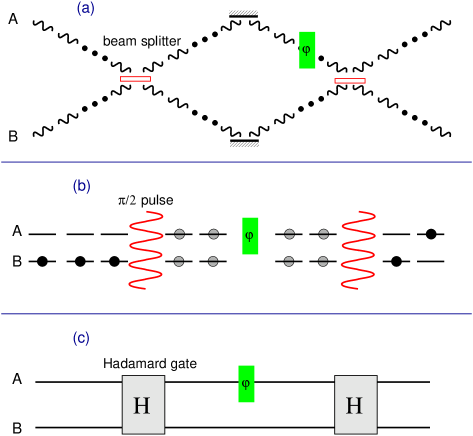
FIG. 1.: The quantum Rosetta stone. (a) An optical Mach-Zehnder interferometer. (b) Ramsey atomic clock. (c) A quantum logic gate representing the equivalent physical proccess.

A third system is given by a qubit that undergoes a Hadamard transform $H$, then picks up a relative phase and is then transformed back with a second Hadamard transformation (Fig. 1c). This representation is more mathematical than the previous two, and it allows us to extract the unifying mathematical principle that connects the three systems. In all protocols, the initial state is transformed by a discrete Fourier transform (beam splitter, $\pi/2$-pulse or Hadamard), then picks up a relative phase, and is transformed back again. This is the standard “quantum” finite Fourier transform, such as used in the implementation of Shor’s algorithm [26]. It is not the same as the classical algorithm in engineering.

As a consequence, the phase shift (which is hard to measure directly) is applied to the transformed basis. The result is a bit flip in the initial, computational, basis $\{|0\rangle,|1\rangle\}$, and this is readily measured. We call the formal analogy between these three systems the quantum Rosetta stone.

The importance of the Rosetta stone was that, by giving an example of writing in three different languages: Greek, Demotic, and Hieroglyphics, it enabled the French scholar Jean François Champollion to crack the code of the hieroglyphs, which was not understood until his work in 1822 [27]. In discussing quantum computer circuits with researchers from the fields of quantum optics or atomic clocks, we find the “quantum Rosetta stone” a useful tool to connect those areas of research to the language of quantum computing – which can be as indecipherable as hieroglyphs to such researchers.

These schemes can be generalized from measuring a simple phase shift to evaluating the action of a unitary transformation $U_{f}$ associated with a complicated function $f$ on multiple qubits. Such an evaluation is also known as a quantum computation. Quantum computing with generalized Mach-Zehnder interferometers has been proposed by Milburn [28], and later linear optics quantum computation has been suggested by Cerf, Adami, and Kwiat [29]. Recently, Knill, Laflamme and Milburn demonstrated an efficient linear optics quantum computation [30]. Implementations of quantum logic gates have also been proposed by using atoms and ion traps [31, 32, 33, 34]. According to our Rosetta stone, the concept of quantum computers is therefore to exploit quantum interference in obtaining the outcome of a computation of $f$. In this light, a quantum computer is nothing but a (complicated) multiparticle quantum interferometer [35, 36].

This logic may also be reversed: a quantum interferometer is therefore a (simple) quantum computer. Often, when discussing, Heisenberg-limited interferometry with complicated entangled states, one encounters the critique that such states are highly susceptible to noise and even one or a few uncontrolled interactions with the environment will cause sufficient degradation of the device and recover only the shot-noise limit [37]. Apply the quantum Rosetta stone by replacing the term “quantum interferometer” with “quantum computer” and we recognize the exact same critique that has been leveled against quantum computers for years. However, for quantum computers, we know the response–to apply quantum error-correcting techniques and encode in decoherence free subspaces. Quantum interferometry is just as hard as quantum computing! The same error-correcting tools that we believe will make quantum computing a reality, will also be enabling for quantum interferometry.

III Quantum enhancement in phase measurements

There have been various proposals for achieving Heisenberg-limited sensitivity, corresponding to different physical realizations of the state $|\varphi_{N}\rangle$ and observable $\hat{A}_{N}$ in Eq. (11). Here, we discuss three different approaches, categorized according to the different quantum states. We distinguish Yurke states, dual Fock states, and maximally entangled states.

A Yurke states

By utilizing the $su(2)$ algebra of spin angular momentum, Yurke et al. have shown that, with a suitably correlated input state, the phase sensitivity can be improved to $1/N$ [4, 5]. Similarly, Hillery and Mlodinow, and Brif and Mann have proposed using the so-called minimum uncertainty state or the “intelligent state”. The minimum uncertainty state is defined as $\Delta J_{x}\Delta J_{y}=|\langle{\hat{J}}_{z}\rangle|/2$, and such a state with $\Delta J_{y}\rightarrow 0$ can yield the Heisenberg limited sensitivity under certain conditions [38, 39].

Let ${\hat{a}}^{\dagger}$, ${\hat{b}}^{\dagger}$ denote the creation operators for the two input modes in Fig. 1a. In the Schwinger representation, the common eigenstates of ${\hat{J}}^{2}$ and ${\hat{J}}_{z}$ are the two-mode Fock states $|j,m\rangle=|j+m\rangle_{A}|j-m\rangle_{B}$, where

$${\hat{J}}_{x} = ({\hat{a}}^{\dagger}{\hat{b}}+{\hat{b}}{\hat{a}}^{\dagger})/2\;;\quad{\hat{J}}_{y}=-i({\hat{a}}^{\dagger}{\hat{b}}-{\hat{b}}{\hat{a}}^{\dagger})/2\;;$$ (13)

$${\hat{J}}_{z} = ({\hat{a}}^{\dagger}{\hat{a}}-{\hat{b}}^{\dagger}{\hat{b}})/2\;;\quad{\hat{J}}^{2}={\hat{J}}_{x}^{2}+{\hat{J}}_{y}^{2}+{\hat{J}}_{z}^{2}\;.$$ (14)

The interferometer can be described by the rotation of the angular momemtum vector, where ${\hat{a}}^{\dagger}{\hat{a}}+{\hat{b}}^{\dagger}{\hat{b}}=N=2j$, and the 50/50 beam splitters and the phaser shift are corresponding to the operators $e^{i\pi{\hat{J}}_{x}/2}$ and $e^{i\varphi{\hat{J}}_{z}}$, respectively.

For spin-1/2 fermions, the entangled input state (which we call the ‘Yurke state’) $|\varphi_{N}\rangle_{\rm Y}$ is given by

$$|\varphi_{N}\rangle_{\rm Y} = {1\over\sqrt{2}}\left[\left|j=\mbox{$\frac{N}{2}$},m=\mbox{$\frac{1}{2}$}\right\rangle+\left|j=\mbox{$\frac{N}{2}$},m=-\mbox{$\frac{1}{2}$}\right\rangle\right]$$ (15)

$$= {1\over\sqrt{2}}\left[\left|\mbox{$\frac{N+1}{2}$},\mbox{$\frac{N-1}{2}$}\right\rangle_{AB}+\left|\mbox{$\frac{N-1}{2}$},\mbox{$\frac{N+1}{2}$}\right\rangle_{AB}\right],$$ (16)

where the notion of $|j,m\rangle$ follows the definition given in Eq. (14) and the subscripts $AB$ denote the two input modes. For bosons, a similar input state, namely $|j=N/2,m=0\rangle+|j=N/2,m=1\rangle$, has been proposed [5]. The measured observable $\hat{A}_{N}$ is given by ${\hat{J}}_{z}$. After evolving the state $|\varphi_{N}\rangle_{\rm Y}$ (in the Ramsey spectroscope or the Mach-Zehnder interferometer with phase shift $\varphi$), the phase sensitivity $\Delta\varphi$ can be determined to be proportional to $1/N$ for special values of $\varphi$ (Fig. 2a). Although the input state of Eq. (16) was proposed for spin-1/2 fermions, the same state with bosons also yields the phase sensitivity of the order of $1/N$ [12].

B Dual Fock states

In order to achieve Heisenberg-limited sensitivity, Holland and Burnett proposed the use of so-called dual Fock states $|N\rangle_{A}\otimes|N\rangle_{B}$ for two input modes $A$ and $B$ of the Mach-Zehnder interferometer [8]. Such a state can be generated, for example, by degenerate parametric down conversion, or by optical parametric oscillation [40].

To obtain increased sensitivity with dual Fock states, some special detection scheme is needed. In a conventional Mach-Zehnder interferometer only the difference of the number of photons at the output is measured. Similarly, in atom interferometers, measurements are performed by counting the number of atoms in a specific internal state using fluorescence. For the schemes using dual Fock-state input, an additional measurement is required since the average in the intensity difference of the two output ports does not contain information about the phase shift (Fig. 2b).

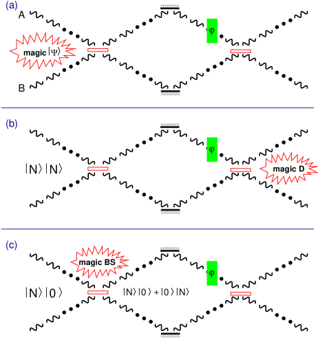
FIG. 2.: Three catagories for achieving the Heisenberg limited phase sensitivity. Emphasis on the distinctive features are termed as “magic”. (a) Correlated input state (magic state), (b) dual Fock-state input (magic detectors), (c) maximally correlated state (magic beam splitter).

One measures both the sum and the difference of the photon number in the two output modes [8]. The sum contains information about the total photon number, and the difference contains information about the phase shift. Information about the total photon number then allows for post-processing the information about the photon-number difference. A combination of a direct measurement of the variance of the difference current and a data-processing method based on Bayesian analysis was proposed by Kim et al. [40]. Recently, Wisemen and co-workers have proposed an adaptive measurement scheme, where the optimal input state, however, is different from the dual Fock states [41].

For atom interferometers, a quantum nondemolition measurement is required to give the total number of atoms [10]. In a similar context, Yamamoto and co-workers devised an atom interferometry scheme that uses a squeezed $\pi/2$ pulse for the readout of the input state correlation [9].

Due to its simple form, the dual Fock-state approach may shed a new light on Heisenberg-limited interferometry. In particular, exploiting the fact that atoms in a Bose-Einstein condensate can be represented by Fock states, Bouyer and Kasevich, as well as Dowling, have shown that the quantum noise in atom interferometry using dual Bose-Einstein consensates can also be reduced to the Heisenberg limit [10, 12].

C Maximally entangled states

The third, and last, category of states is given by the maximally entangled states. There have been proposals to overcome the standard shot noise limit by using spin-squeezed states [42, 43, 44, 45, 46]. However, it was demonstrated by Wineland and co-workers [11] that the optimal frequency measurement can be achieved by using maximally entangled states [47], which have the following form:

$$|\varphi_{N}\rangle=\frac{1}{\sqrt{2}}\left(\left|N,0\right\rangle_{AB}+\left|0,N\right\rangle_{AB}\right)\;.$$ (17)

This state has an immediate resemblence with the state in Eq. (11) after acquiring a phase shift of $e^{iN\varphi}$. Although partially entangled states with a high degree of symmetry were later shown to have a better resolution in the presence of decoherence [48], these maximally correlated states are of great interest for optical interferometry.

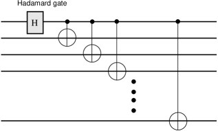
FIG. 3.: Quantum logic gates for generation of the maximally entangled states (representing the “magic” beam splitter in Fig. 2c). $N$ qubits become maximally entangled via a Hadamard gate followed by $N$ C-NOT gates.

In terms of quantum logic gates, the maximally correlated state of the form of Eq. (17) can be made using a Hadamard gate and a sequence of C-NOT gates (see Fig. 3). Note that one distinctive feature, compared to the other schemes described above, is that the state of the form Eq. (17) is the desired quantum state after the first beam splitter in the Mach-Zehnder interferometer, not the input state (Fig. 2c). In that the desired input state is described as the inverse beam-splitter operation to the state of Eq. (17).

All the interferometric schemes using entangled or dual-Fock input states show a sensitivity approaching $1/N$ only asymptotically. However, using the maximally correlated states of Eq. (17), the phase sensitivity is equal to $1/N$, even for a small $N$.

IV Quantum lithography and maximally path-entangled states

Quantum correlations can also be applied to optical lithography. In recent work it has been shown that the Rayleigh diffraction limit in optical lithography can be circumvented by the use of path-entangled photon number states [13, 14]. The desired $N$-photon path-entangled state, for $N$-fold resolution enhancement, is again of the form given in Eqs. (8) and (17).

Consider the simple case of a two-photon Fock state $|1\rangle_{A}|1\rangle_{B}$, which is a natural component of a spontaneous parametric down-conversion event. After passing through a 50/50 beam splitter, it becomes an entangled number state of the form $|2\rangle_{A}|0\rangle_{B}+|0\rangle_{A}|2\rangle_{B}$. Interference suppresses the probability amplitude of $|1\rangle_{A}|1\rangle_{B}$. According to quantum mechanics, it is not possible to tell whether both photons took path $A$ or $B$ after the beam splitter.

When parametrizing the position $x$ on the surface by $\varphi=\pi x/\lambda$, the deposition rate of the two photons onto the substrate becomes $1+\cos 2\varphi$, which has twice better resolution $\lambda/8$ than that of single-photon absorption, $1+\cos\varphi$, or that of uncorrelated two-photon absorption, $(1+\cos\varphi)^{2}$. For $N$-photon path-entangled state of Eq. (17), we obtain the deposition rate $1+\cos N\varphi$, corresponding to a resolution enhancement of $\lambda/(4N)$.

It is well known that the two-photon path-entangled state of Eq. (17) can be generated using a Hong-Ou-Mandel (HOM) interferometer [49] and two single-photon input states. A 50/50 beam splitter, however, is not sufficient for producing path-entangled states with a photon number larger than two [50].

As depicted in Fig. 3, the maximally correlated state of the form of Eq. (17) can be made using a Hadamard gate and a sequence of $N$ C-NOT gates. However, building optical C-NOT gates normally requires large optical nonlinearities. Consequently, in generating such states it is commonly assumed that large $\chi^{(3)}$ nonlinear optical components are needed for $N>2$.

Knill, Laflamme, and Milburn proposed a method for creating probabilistic single-photon quantum logic gates based on teleportation. The only resources for this method are linear optics and projective measurements [30]. Probabilistic quantum logic gates using polarization degrees of freedom have been proposed by Imoto and co-workers, and Franson’s team [51, 52]. In particular, Pittman, Jacobs, and Franson have experimentally demonstrated polarization-based C-NOT implementations [53].

Using the concept of projective measurements, we have previously demonstrated that the desired path-entangled states can be created when conditioned on the measurement outcome [19, 54]. This way, one can avoid the use of large $\chi^{(3)}$ nonlinearities [55]. In the next section we discuss the path-entanglement generation based on projective measurements, and its application to Heisenberg-limited interferometry.

V Projective measurements and Heisenberg-limited interferometry

As is discussed in the previous sections, the Yurke state approach has the same measurement scheme as the conventional Mach-Zehnder interferometer (direct detection of the difference current), but it is not easy to generate the desired correlation in the input state [12]. On the other hand, the dual Fock-state approach finds a rather simple input state, but requires a complicated measuremet schemes. In this section we describe a method for creating a desired correlation in the Yurke state approach directly from the dual Fock state by using the projective measurements.

Consider the scheme depicted in Fig. 4. The input modes are transformed by the beam splitters as follows:

$${\hat{a}}^{\dagger} \rightarrow it{\hat{a}}^{\prime\dagger}+r{\hat{u}}^{\prime\dagger},$$ (18)

$${\hat{b}}^{\dagger} \rightarrow it{\hat{b}}^{\prime\dagger}+r{\hat{v}}^{\prime\dagger},$$ (19)

where $i=\sqrt{-1}$, and $it$ and $r$ are the transmission and reflection coefficients given by $t^{2}+r^{2}=1$. In our convention, a 50/50 beam splitter, for example, is identified as $t=1/\sqrt{2}$ and $r=-1/\sqrt{2}$.

The modes ${\hat{u}}^{\prime}$ and ${\hat{v}}^{\prime}$ further pass through an additional 50/50 beam splitter, which is characterized by the transformations:

$${\hat{u}}^{\prime\dagger} \rightarrow(i{\hat{d}}^{\dagger}-{\hat{c}}^{\dagger})/\sqrt{2},$$ (20)

$${\hat{v}}^{\prime\dagger} \rightarrow(i{\hat{c}}^{\dagger}-{\hat{d}}^{\dagger})/\sqrt{2}.$$ (21)

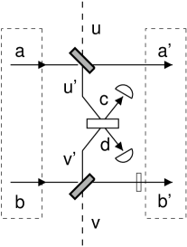
FIG. 4.: If one and only one photon is detected at each detector, two photons are “peeled off” from either input mode $a$ or $b$.

Suppose the input state is given by the dual Fock state

$$|\Psi_{\rm in}\rangle=|N,N\rangle={({\hat{a}}^{\dagger})^{N}({\hat{b}}^{\dagger})^{N}\over N!}|0\rangle\;.$$ (22)

Accordingly, the beam splitter transformation, e.g., for the mode $a$, can be written as

$$({\hat{a}}^{\dagger})^{N} \rightarrow \sum_{k}~{}_{N}C_{k}({\hat{a}}^{\prime\dagger})^{N-k}({\hat{u}}^{\prime\dagger})^{k}r^{k}(it)^{N-k}\;.$$ (23)

Let both modes pass through a beam splitter, and recombine the reflected modes $u^{\prime}$ and $v^{\prime}$ in a 50/50 beam splitter as depicted in Fig. 4. We post-select events on a two-fold detector coincidence at the output modes of this beam splitter. Assuming ideal detectors, this will restrict the final state of the outgoing modes $a^{\prime}$ and $b^{\prime}$. Then, from Eq. (21), we have

$${\hat{u}}^{\prime\dagger}{\hat{v}}^{\prime\dagger} \rightarrow-i\left[({\hat{c}}^{\dagger})^{2}+({\hat{d}}^{\dagger})^{2}\right]/2\;,$$ (24)

$$({\hat{u}}^{\prime\dagger})^{2} \rightarrow\left[({\hat{c}}^{\dagger})^{2}-2i{\hat{c}}^{\dagger}{\hat{d}}^{\dagger}-({\hat{d}}^{\dagger})^{2}\right]/2\;,$$ (25)

$$({\hat{v}}^{\prime\dagger})^{2} \rightarrow\left[-({\hat{c}}^{\dagger})^{2}-2i{\hat{c}}^{\dagger}{\hat{d}}^{\dagger}+({\hat{d}}^{\dagger})^{2}\right]/2\;.$$ (26)

We note that only $({\hat{u}}^{\prime\dagger})^{2}$ and $({\hat{v}}^{\prime\dagger})^{2}$ terms are selected by the detection of a single photon at each detector. The output state conditioned on a two-fold coincident count is given by

$$|N,N\rangle\rightarrow{A\over\sqrt{2}}\left[|N,N-2\rangle+|N-2,N\rangle\right]\;,$$ (27)

where $A=\sqrt{N(N-1)/2}~{}r^{2}t^{2N-2}$, and the maximum probability success is obtained when $r^{2}={1\over N}$ and, $t^{2}={N-1\over N}$. The output state of the form Eq. (27) shows the exact correlation for the Yurke state [12]. The generation of the desired correlations described in section III A can thus be obtained from the dual Fock state $|N,N\rangle$ with probability $|A|^{2}$. Note that this probability has its asymptotic value of $1/(2e^{2})$, independent of $N$.

A similar correlation can also be ontained by post selecting the outcome, conditioned upon only one photon detection by either one of the two detectors. The analysis becomes simpler than the one decribed above: one photon either from mode $a$ or from $b$ is to be detected. In this case, however, one needs to allow a non-detection protocol [19] since one of the two detectors should not be fired.

In this section we described generation of quantum correlation by using projective measurments, where the fundamental lack of which-path information provides the entanglement between the two output modes. Using a stack of such devices with appropriate phase shifters has been proposed for generating maximmally path-entangled state of the form Eq. (17) [19]. In atom interferometry a similar technique for the the generation of such a correlation has been proposed [12] with selective measurements on two interfering Bose condensates [56].

VI summary

In this paper we discuss the equivalence between the optical Mach-Zehnder interferometer, the Ramsey spectroscope, and the quantum Fourier transform in the form of a specific quantum logic gate. Based on this equivalence, we introduce the so-called quantum Rosetta stone.

The interferometers and spectroscopes can yield Heisenberg-limited phase sensitivity when suitable input states are chosen. We presented three types of such states and showed that they need non-local correlations of some sort. Path-entangled multi-photon states can be generated using projective measurements. These states yield $1/N$ sensitivity also for small $N$, and are essential for applications such as quantum lithography. The dual Fock-state approach to Heisenberg-limited interferometry must be accompanied by “non-local” detection schemes. The generation of a suitable correlation from the dual Fock state via projective measurements may be useful in that it avoids complicated signal processing or quantum nondemolition measurements. One can also construct a single-photon quantum nondemolition device and a quantum repeater in this paradigm [57, 58]. Many more important insights are expected by the application of the quantum Rosetta stone to quantum metrology and quantum information processing.

REFERENCES

- [1] For example, see, M.O. Scully and M.S. Zubairy, Quantum Optics (Cambridge University Press, Cambridge, UK, 1997).
- [2] C.W. Helstrom, Quantum detection and estimation theory, Mathematics in Science and Engineering 123 (Academic Press, New York, 1976).
- [3] C.M. Caves, Phys. Rev. D 23, 1693 (1981).
- [4] B. Yurke, Phys. Rev. Lett. 56, 1515 (1985).
- [5] B. Yurke, S.L. McCall, and J.R. Klauder, Phys. Rev. A 33, 4033 (1986).
- [6] B.C. Sanders and G.J. Milburn, Phys. Rev. Lett. 75, 2944 (1995).
- [7] Z.Y. Ou, Phys. Rev. Lett. 77, 2352 (1996).
- [8] M.J. Holland and K. Burnett, Phys. Rev. Lett. 71, 1355 (1993).
- [9] J. Jacobson, G. Björk, Y. Yamamoto, Appl. Phys. B 60, 187 (1995).
- [10] P. Bouyer and M.A. Kasevich, Phys. Rev. A 56, R1083 (1997).
- [11] J.J. Bollinger et al., Phys. Rev. A 54, R4649 (1996).
- [12] J.P. Dowling, Phys. Rev. A 57, 4736 (1998).
- [13] E. Yablonovich and R.B Vrijen, Opt. Eng. 38, 334 (1999).
- [14] A.N. Boto et al., Phys. Rev. Lett. 85, 2733 (2000).
- [15] P. Kok et al., Phys. Rev. A 63, 063407 (2001).
- [16] G.S. Agarwal et al., Phys. Rev. Lett. 86, 1389 (2001).
- [17] M. D’Angelo et al., Phys. Rev. Lett. 87, 013602 (2001).
- [18] E.M. Nagasako et al., Phys. Rev. A 64, 043802 (2001).
- [19] P. Kok, H. Lee, and J.P. Dowling, “The creation of large photon-number path entanglement conditioned on photodetection,” Phys. Rev. A (in press), quant-ph/0112002.
- [20] Z. Hradil, Quant. Opt. 4, 93 (1992).
- [21] A.S. Lane, S.L. Braunstein, and C.M. Caves, Phys. Rev. A 47, 1667 (1993).
- [22] The discussion about the Mach-Zehnder is equally applicable to the Fabry-Perot interferometer.
- [23] R.P. Feynman, R.B. Leighton, and M. Sands, The Feynman Lectures on Phyisics III (Addison-Wesley, Reading, MA, 1979).
- [24] B.-G. Englert, J. Schwinger, and M.O. Scully, Found. Phys. 18, 1045 (1988); J. Schwinger, M.O. Scully, and B.-G. Englert, Z. Phys. D 10, 135 (1988); M.O. Scully, B.-G. Englert, and J. Schwinger, Phys. Rev. A 40, 1775 (1989).
- [25] M.O. Scully and J.P. Dowling, Phys. Rev. A 48, 3186 (1993).
- [26] A. Ekert and R. Jozsa, Rev. Mod. Phys. 68, 733 (1996).
- [27] J.F. Champollion, Précis du système hiéroglyphique des anciens Egyptiens (Paris, 1824).
- [28] G.J. Milburn, Phys. Rev. Lett. 62, 2124 (1989).
- [29] N.J. Cerf, C. Adami, and P.G. Kwiat, Phys. Rev. A 57, R1477 (1998).
- [30] E. Knill, R. Laflamme, and G.J. Milburn, Nature 409, 46 (2001).
- [31] P. Domokos et al., Phys. Rev. A 52, 3554 (1995).
- [32] J.I. Cirac and P. Zoller, Phys. Rev. Lett. 74, 4091 (1995).
- [33] Q. A. Turchette et al., Phys. Rev. Lett. 75, 4710 (1995).
- [34] C. Monroe et al., Phys. Rev. Lett. 75, 4714 (1995).
- [35] A. Ekert, Physica Scripta T76, 218 (1998).
- [36] R. Cleve, et al., Proc. R. Soc. Lond. A 454, 339 (1998).
- [37] H. J. Kimble, private communication.
- [38] M. Hillery and L. Mlodinow, Phys. Rev. A 48, 1548 (1993).
- [39] C. Brif and A. Mann, Phys. Rev. A 54, 4505 (1996).
- [40] T. Kim et al., Phys. Rev. A 57, 4004 (1998).
- [41] D.W. Berry and H.M. Wiseman, Phys. Rev. Lett. 85, 5098 (2000); D.W. Berry, H.M. Wiseman, and J.K. Breslin, Phys. Rev. A 63, 053804 (2001).
- [42] M. Kitagawa and M. Ueda, Phys. Rev. Lett. 67, 1852 (1993).
- [43] D.J. Wineland et al., Phys. Rev. A 46, R6797 (1992).
- [44] M. Kitagawa and M. Ueda, Phys. Rev. A 47, 5138 (1993).
- [45] W.M. Itano et al., Phys. Rev. A 47, 3554 (1993).
- [46] G.S. Agarwal and R.R. Puri, Phys. Rev. A 49, 4968 (1994).
- [47] N.D. Mermin, Phys. Rev. Lett. 65, 1838 (1990).
- [48] S.F. Huelga et al., Phys. Rev. Lett. 79, 3865 (1997); S.F. Huelga et al., Appl. Phys. B 67, 723 (1998).
- [49] C.K. Hong, Z.Y. Ou, and L. Mandel, Phys. Rev. Lett. 59, 2044 (1987).
- [50] R.A. Campos, B.E.A. Saleh, and M.C. Teich, Phys. Rev. A 40, 1371 (1989).
- [51] M. Koashi, T. Yamamoto, and N. Imoto, Phys. Rev. A 63, 030301 (2001).
- [52] T.B. Pittman, B.C. Jacobs, and J.D. Franson, Phys. Rev. A 64, 062311 (2001).
- [53] T.B. Pittman, B.C. Jacobs, and J.D. Franson, “Demonstration of Non-Deterministic Quantum Logic Operations using Linear Optical Elements,” quant-ph/0109128.
- [54] H. Lee, P. Kok, N.J. Cerf, and J.P. Dowling, Phys. Rev. A 65, 030101 (R) (2002).
- [55] C. Gerry and R.A. Campos, Phys. Rev. A 64, 063814 (2001).
- [56] Y. Castin and J. Dalibard, Phys. Rev. A 55, 4330 (1997).
- [57] P. Kok, H. Lee, and J.P. Dowling, “Implementing a single-photon quantum nondemolition device with only linear optics and projective measurements,” quant-ph/0202046.
- [58] P. Kok, C.P. Williams, and J.P. Dowling, “Practical quantum repeaters with linear optics and double-photon guns,” quant-ph/0203134.