Direct Measurement of the Photon Statistics of a Triggered Single Photon Source

Abstract

We studied intensity fluctuations of a single photon source relying on the pulsed excitation of the fluorescence of a single molecule at room temperature. We directly measured the Mandel parameter $Q(T)$ over 4 orders of magnitude of observation timescale $T$, by recording every photocount. On timescale of a few excitation periods, subpoissonian statistics is clearly observed and the probablility of two-photons events is 10 times smaller than Poissonian pulses. On longer times, blinking in the fluorescence, due to the molecular triplet state, produces an excess of noise.

Over the past few years, there has been a growing interest for generating a regular stream of single photons on demand. This was mainly motivated by applications in the field of quantum cryptography Gisin et al. (2001). An ideal single photon source (SPS) should produce light pulses containing exactly one photon per pulse, triggered with a repetition period $\tau_{\rm rep}$, and delivered at the place of interest with 100% efficiency. For any given measurement time $T$, this source would emit exactly $N=T/\tau_{\rm rep}$ photons, so that the standard deviation $\Delta N\equiv\sqrt{\langle N^{2}\rangle_{T}-\langle N\rangle_{T}^{2}}=0$ ($\langle\;\rangle_{T}$ has to be understood as a mean value over a set of measurements lasting $T$). Such a source would then be virtually free of intensity fluctuations, therefore corresponding to perfect intensity squeezing Reynaud (1990).

A first category of SPSs already realized consists of sources operating at cryogenic temperature. They rely on optically Kim et al. (1999); Michler et al. (2000); Santori et al. (2001); Moreau et al. (2001) or electrically Yuan et al. (2002) pumped semiconductor nanostructures or on the fluorescence of a two level system coherently prepared in its excited state Brunel et al. (1999). A one–atom micromaser has also been used to prepare arbitrary photon number states on demand Brattke et al. (2001). However the collection efficiency of photons is barely higher than a few $10^{-3}$ in these experiments. Due to this very strong attenuation, the intensity statistics are very close to a Poisson law at the place where the stream of photons is available. Another route is to realize SPSs at room temperature. In this case higher collection efficiency (around 5%) is achieved. The existing room–temperature SPSs rely on the pulse saturated emission of a single 4–levels emitter Martini et al. (1996); Brouri et al. (2000).

When the pulse duration $\tau_{\rm p}$ is much shorter than the dipole radiative lifetime $\tau_{\rm rad}$, such a single emitter can only emit one photon per pulse. This temporal control of the dipole excitation allows therefore to easily produce individual photons on demand Lounis and Moerner (2000); Beveratos et al. (2002). However, in previous SPS realizations, little attention has been paid to analyse their intensity fluctuations. To address this problem we realized a room–temperature SPS relying on the pulsed saturation of a single molecule embedded in a thin polymer film Treussart et al. (2001).

The samples are made of cyanine dye DiIC₁₈(3) molecules dispersed at a concentration of about one molecule per 10 $\mu m^{2}$ into a 30 nm thick PMMA layer, spincoated over a microscope coverplate. The fluorescence from the single molecule is excited and collected by the standard technique of scanning confocal optical microscopy Nie and Zare (1997). The molecules are non–resonantly excited at 532 nm, with femtosecond pulses generated by a Ti:Sapphire laser and frequency doubled by single pass propagation into a LiIO₃ crystal. The repetition rate, initially at 82 MHz, is divided by a pulsepicker. The energy per pulse $E_{\rm p}$ is adjustable by an electro–optic modulator. The pulse duration is about $\tau_{\rm p}\approx 100$ fs. The excitation light is reflected by the dichroic mirror of an inverted microscope, and then focused by an oil–immersion objective ($\times 60$, NA=1.4), to form a spot of $\approx 1\mu$m² surface area. The fluorescence light from the sample is collected by the same objective and then focused into a 30 $\mu$m diameter pinhole. After recollimation, a holographic notch filter removes the residual pump light. A standard Hanbury Brown and Twiss (HBT) setup is then used to split the beam and detect single photons on two identical avalanche photodiodes. Glass filters are placed onto each arm to suppress parasitic crosstalk Kurtsiefer et al. (2001) between the two photodiodes.

In order to rapidly identify single molecule emission, we first measure the intensity autocorrelation function $\langle I(t)I(t+\tau)\rangle$ of the fluorescence light by the standard Start–Stop technique with a time–to–amplitude converter Brunel et al. (1999). When a single emitter is addressed, there is virtually no event registered at $\tau=0$, since a single photon cannot be simultaneously detected on both sides of a beamsplitter Grangier et al. (1986). The histogram shows a peak pattern at the pulse repetition period $\tau_{\rm rep}$. As explained in Ref.Brunel et al. (1999), the peaks’ areas allow one to infer the probabilities $P_{\rm S}(n)$ for the source (S), of giving $n=0,1,2$ photocounts per excitation pulse, where 2 photons counts are due to deviation from the ideal SPS. Nevertheless, this technique can hardly be used to extract the intensity fluctuations on timescale longer than a single pulse. We have therefore chosen to record each photodetection event with a two–channel Time Interval Analyser computer board (GuideTech, Model GT653). Since each detection channel has a deadtime of 250 ns the excitation repetition rate was chosen to be 2 MHz.

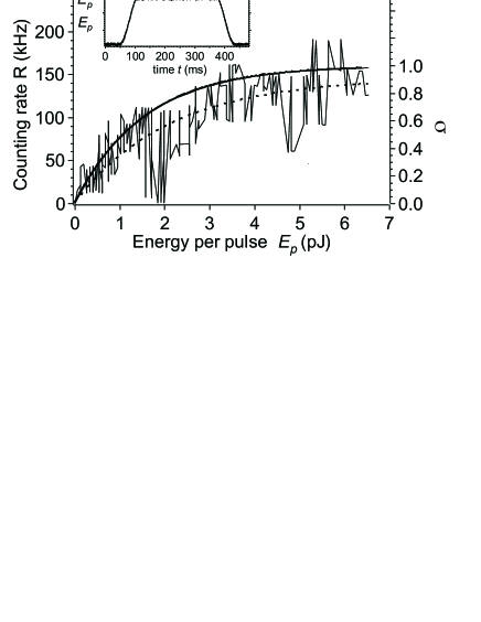
Figure 1: Photon counting rate $R$ vs. energy per pulse, for a single molecule. The inset shows the excitation ramp $E_{\rm p}(t)$, with $E_{\rm p}^{\rm max}=13$ pJ in this case. The record of the saturation curve was limited by the photobleaching of the dye. The dashed curve is a fit of the raw data according to eq.(1) and the solid line is a fit after correction of triplet state excursion. The right scale shows the excited state population $\sigma$.

In a typical experiment, we first raster scan the sample at low excitation energy per pulse (0.5 pJ). When a single molecule is located, we apply the excitation energy ramp $E_{\rm p}(t)$ shown on inset of Fig.1, and simulteaneously record the fluorescence counts on a 1 ms integration time. Fig.1 displays the fluorescence counting rate $R$ vs. $E_{\rm p}$. The large intensity fluctuations are due to triplet state excursion of the molecule (see Fig.2). If this state is not taken into account, the molecular energy levels can be modelised by a 2-level system assuming a very fast non-radiative relaxation between the two higher and the two lower energy states. The excited state population $\sigma$ at the time $\tau_{\rm p}$ after the pulse arrival is then

$$\sigma={E_{\rm p}/E_{\rm sat}\over{(1+E_{\rm p}/E_{\rm sat})}}\left(1-e^{-{\tau_{\rm p}\over\tau_{\rm rad}}\left(1+{E_{\rm p}\over E_{\rm sat}}\right)}\right),$$ (1)

where $\tau_{\rm rad}\approx 2.8~{}$ns for the cyanine considered. The data $R(E_{\rm p})$ are fitted by the function $R=R_{0}\times\sigma$ in a two steps procedure. After a first fit of the raw data, all the points below this fit, which are attributed to triplet state excursion, are removed. The fit of the remaining set of data yields $R_{0}=160\times 10^{3}$ counts/s and $E_{\rm sat}=5.6\times 10^{-5}$ pJ.

In order to optimize the number of emitted photons and avoid rapid photobleaching, we then set $E_{\rm p}^{\rm max}$ to 5.6 pJ. Such a value would correspond to $\sigma=97\%$, for the molecule studied in Fig.1. During the constant maximum pumping energy period of the excitation ramp, $10^{4}$ detection events are typically recorded before photobleaching. Thanks to the high stability of the period of the pulsed laser, this set of times can be synchronized on an excitation timebase. We then build the table of the number of photocounts $n_{i}=0,1,2$ for each excitation pulse $i$. Photons which are delayed by more than $10\times\tau_{\rm rad}$ are considered to come from the dark counts of the two photodiodes, and are therefore rejected.

X	$P_{\rm X}(1)$	$P_{\rm X}(2)$	$\overline{n}_{\rm X}$	$V-1$
S	0.0466	$5.0\times 10^{-5}$	0.0467	-0.0445
R	0.0452	$50\times 10^{-5}$	0.0462	-0.0244
C	0.0451	$53\times 10^{-5}$	0.0462	-0.0231

Table 1: Photocount probabilities $P_{\rm X}(n),\;n=1,2$, of our SPS (X=S), of an experimental reference source (R) and of a theoretical coherent source (C), the photocount statistics of which is affected by the detection setup. $\overline{n}_{\rm X}$ are the mean number of detected photons per pulse and $V$, the normalized variances. Negative values of $V$ for the coherent and reference sources are due to a dead time effect.

The data considered hereafter corresponds to a molecular source (S) which survived during 319769 periods (about 160 ms) yielding 14928 recorded photons including 14896 single photon events, 16 two-photons events. We deduced $P_{\rm S}(1)=0.0466$ and $P_{\rm S}(2)=5.0\times 10^{-5}$ and a mean number of detected photon per pulse $\overline{n}_{\rm S}=0.0467$ (see Table 1). The real source is considered as the superposition of an attenuated ideal SPS with an overall quantum efficiency $\eta$, and a coherent source simulating the background, which adds a mean number of detected photon per pulse $\gamma$. From the measured values of $P_{\rm S}(1)$ and $P_{\rm S}(2)$, we infer $\eta\approx 0.0445$ and $\gamma\approx 2.2\times 10^{-3}$. This leads to a signal-to-background ratio of about 20.

We also compared experimentally our SPS to a reference source (R) made of attenuated pump laser pulses, with approximately the same mean number of detected photons per pulse. Quantitative tests of this reference source and of the detection setup are however necessary. A particular care has to be taken to the bias of photocount statistics due to the detection deadtimes on both channels. For a coherent state of light (C) containing $\alpha$ photon per excitation pulse, one can readily calculate the counting probability distribution and show that $\displaystyle P_{\rm C}(0)=e^{-\alpha},P_{\rm C}(1)=2e^{-\alpha/2}(1-e^{-\alpha/2})$, $\displaystyle P_{\rm C}(2)=(1-e^{-\alpha/2})^{2}$ and $\overline{n}_{\rm C}=2(1-e^{-\alpha/2})$, where $\overline{n}_{\rm C}$ is the mean number of detected photons per pulse. For the reference source (R), we measured $\overline{n}_{\rm R}=0.0462$, $P_{\rm R}(1)=0.0452$, $P_{\rm R}(2)=50\times 10^{-5}$, whereas one predicts, for $\overline{n}_{\rm C}=\overline{n}_{\rm R}$, $P_{\rm C}(1)=0.0451$ and $P_{\rm C}(2)=53\times 10^{-5}$. The measured values are in good agreement with the predictions, which proves that the faint Ti:Sapphire pulses make a good calibration source for Poisson statistics. We then infer the ratio $P_{\rm S}(2)/P_{\rm R}(2)=0.10$, which tells that the number of two photons pulses in our SPS, is 10 times smaller than in the reference poissonian source (R).

In a first attempt to estimate the fluorescence intensity fluctuations per pulse, we considered samples of the data made of $W$ excitation cycles. We introduced a normalized variance $V_{\rm W}$ defined, on the sample, by $V_{W}\equiv\langle(\Delta n)^{2}\rangle_{\rm w}/\langle n\rangle_{\rm w}$, with $\langle(\Delta n)^{2}\rangle_{\rm w}\equiv\sum_{i=1}^{W}(n_{i}-\langle n\rangle_{\rm w})^{2}/W$, where $n_{i}$ is the number of detected photons for the pulse $i$ and $\langle n\rangle_{\rm w}$ is the mean number of detected photon per pulse in the sample considered. In the very few samples for which $\langle n\rangle_{\rm w}=0$, $V_{W}$ is not defined and is set to 1. For a Poisson distribution of photocounts $V_{W}=1$, whereas $V_{W}<1$ for subpoissonian distribution.

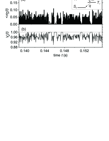
Figure 2: (a) Mean number $\langle n\rangle_{\rm w}$ of photons detected in successive samples of the data of constant size $W=100$ cycles (bin period of $50~{}\mu$s). (b) Corresponding time trace of the normalised variance $V_{\rm w}$ showing reduction of noise ($V_{\rm w}<1$) during the emission period of the molecule. Inset of (a) displays the molecular level diagram.

In order to follow the time evolution of intensity fluctuations, we then extract from the set of $\{n_{i}\}$ all the successive samples of photocounts measurements of size $W=100$, separated by a single pulse period. Fig.2(a) displays the mean number of detected photons per pulse vs. time. We clearly see random intermittency in the fluorescence of the molecule, due to the presence of a dark triplet state $T_{1}$ in the molecular energy levels diagram (see inset of Fig.2(a)). At each excitation cycle the molecule has a small probability to jump into this non–fluorescent state, where it stays for a time much longer than the repetition period. Fig.2(b) shows, in parallel, the timetrace $V_{W}(t)$ of the normalized variance. During an emission period, $V_{W}$ stays below 1, and the statistics of the number of the detected photons per pulse is subpoissonian. On the other hand, when the molecule stops to emit, the background light yields $V_{W}\approx 1$. If we now consider the whole set of data, our measurements yields a single value for the variance $V=0.9555$. In this intensity fluctuation analysis at the level of a single pulse, this value of $V$ is also directly related to the Mandel paramater Loudon (2000) $Q\equiv\langle(\Delta n)^{2}\rangle/\langle n\rangle-1$ by $Q=V-1=-0.0445$. Let us point out that due to the photodetection deadtime, the triggered reference source (R) also yields a subpoissonian counting statistics. More precisely, for the coherent source (C) giving about the same mean number $\overline{n}_{\rm C}$ of photons per pulse than our SPS, one predicts a value $\displaystyle Q=-\overline{n}_{\rm C}/2=-0.0231$. This is confirmed by our measurements on the reference source (see Table 1). Nevertheless, the fluctuations of the number of detected photons per pulse coming out of our SPS show a clear departure from the reference coherent source. Albeit still limited by the quantum efficiency $\eta$, this direct measurement of $|Q|$ is larger by more than one order of magnitude compared to previous experiments Short and Mandel (1983); Diedrich and Walther (1987). For such a solid state SPS like ours, any improvement achieved in the light collection efficiency would therefore yield higher values of this subpoissonian character. We indeed observed, in preliminary experiments, an increase of the collection efficiency by placing the molecule at a controlled distance of a metallic mirror.

However, the leak in the dark triplet state induces correlations between consecutive pulses. The measurement of the variance $V$ of the detected photon number per pulse is therefore insufficient to characterize the noise properties of our SPS. Whereas such a characterization is usually infered from the record of noise power spectra, our photocount measurements are performed in the time domain. We therefore introduce, as a new variable, the number $N(T)=\sum_{i=1}^{k}n_{i}$ of the detected photons during any period of observation $T=k\tau_{\rm rep}$. The analysis of the fluctuations of the variable $n_{i}$ can be generalized to the variable $N(T)$, by using the time dependent Mandel parameter Mandel (1979) $Q(T)\equiv\langle(\Delta N)^{2}\rangle_{T}/\langle N\rangle_{T}-1$. We can also define a Mandel parameter $Q_{\rm s}(T)$ for the number of photons emitted by the source in the same period of time $T$. In the case of an ideal SPS, we have $Q=\eta\times Q_{\rm s}$ Abate et al. (1976). For such a source, $Q_{\rm s}=-1$, and therefore $Q(T)=-\eta$, for any value of $T$.

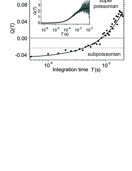
Figure 3: Direct measurements of Mandel parameter $Q(T)$ over short recording time $T$. Dashed line shows $Q(T)$ for the equivalent coherent source (C). Inset shows $Q(T)$ for longer time of observation. The solid curve is a fit to the data by a model accounting for intermittency in the SPS emission.

Fig.3 shows that we did observe subpoissonian intensity fluctuations on timescales from $T=1\times\tau_{\rm rep}$ to $T=8\times\tau_{\rm rep}$, with the minimum value $Q(\tau_{\rm rep})=-0.0445$ achieved on a single pulse timescale, as explained above. When we consider the number of detected photons on timescales larger than $10^{-5}$ s, the intensity fluctuations exhibit a superpoissonnian behaviour ($Q(T)>0$) as shown on inset of Fig.3. This is a direct consequence of the bunching due to the triplet state Bernard et al. (1993). We developped a simple model to account for the intermittency of the SPS emission. In this model, the molecule is either available for fluorescence and is said to be in a ON state, or it is in its triplet OFF state and does not fluoresce. Let us note $p$, the probability per unit of time to make a ON $\rightarrow$ OFF transition, and $q=1/\tau_{\rm T}$ the one to make the reverse OFF $\rightarrow$ ON transition, where $\tau_{\rm T}$ is the lifetime of the triplet state. Note that $p\tau_{\rm rep}=\rm\cal{P}_{\rm ISC}$ is the intersystem crossing probability per excitation pulse. From measured values at the single molecule level with DiIC₁₈(3) cyanine dye Veerman et al. (1999), $p\tau_{\rm rep}\approx 10^{-4}\ll 1$ and $q\tau_{\rm rep}\approx 2.5\times 10^{-3}\ll 1$. In this limiting case, the Mandel parameter of the source is

$$Q_{\rm s}(k\tau_{\rm rep})={{2\times\cal{P}_{\rm ISC}}\over\beta^{2}}\biggl{\{}1-{1\over{k\beta}}\left[1-(1-\beta)^{k}\right]\biggr{\}}-1$$ (2)

where $\beta\equiv(p+q)\tau_{\rm rep}=\cal{P}_{\rm ISC}+\tau_{\rm rep}/\tau_{\rm T}$. The Mandel parameter of the detected photon counts is then $Q(T)=\eta\times Q_{\rm s}(T)$. As shown on Fig.3, our data for $Q(T)$ are well fitted by eq.(2) over more than 4 orders of magnitude, with $\eta=0.0445$ (measured) and the free parameters $p$ and $q$. The fit yields $p\tau_{\rm rep}\approx 2\times 10^{-4}$ and $\tau_{\rm T}\approx 250\,\mu$s, in good agreement with Ref.Veerman et al. (1999).

As a conclusion, the record of every photocount time allows one to make a direct time domain fluctuation analysis, as presented in this Letter. This technique can be straightforwardly applied to other SPS, and is also suited to investigate photochemical propreties at the single molecule level.