Unstable systems and quantum Zeno phenomena in quantum field theory

Abstract

We analyze the Zeno phenomenon in quantum field theory. The decay of an unstable system can be modified by changing the time interval between successive measurements (or by varying the coupling to an external system that plays the role of measuring apparatus). We speak of quantum Zeno effect if the decay is slowed and of inverse quantum Zeno (or Heraclitus) effect if it is accelerated. The analysis of the transition between these two regimes requires close scrutiny of the features of the interaction Hamiltonian. We look in detail at quantum field theoretical models of the Lee type.

1 Introduction

The seminal formulation of the quantum Zeno effect by Misra and Sudarshan[1] deals with unstable systems, i.e. systems that decay following an approximately exponential law.[2] Such a formulation was implicit also in previous work,[3] where the features of the “nondecay” amplitude and probability were investigated. The attention was diverted to oscillating systems, characterized by a finite Poincaré time, when Cook published a remarkable paper,[4] proposing to test the quantum Zeno effect (QZE) on a two-level system undergoing Rabi oscillations. Although oscillating systems are somewhat less interesting in this context, they are also much simpler to analyze and indeed motivated interesting experiments[5] and lively discussions,[6] giving rise to new ideas.[7] However, interesting new phenomena occur when one considers unstable systems, whose Poincaré time is infinite:[8, 9, 10] in particular, other regimes become possible, in which measurement accelerates the dynamical evolution, giving rise to an inverse quantum Zeno effect (IZE).[11, 12, 13, 14]

The study of Zeno effects for bona fide unstable systems requires the use of quantum field theoretical techniques and in particular the Weisskopf-Wigner approximation[15] and the Fermi “golden” rule:[16] for an unstable system the form factors of the interaction play a fundamental role and determine the occurrence of a Zeno or an inverse Zeno regime, depending of the physical parameters describing the system. The occurrence of new regimes is relevant from an experimental perspective, in view of the beautiful experiments recently performed by Raizen’s group on the short-time non-exponential decay (leakage through a confining potential)[17] and on the Zeno effects for such (nonoscillating) systems.[18]

We analyze here the transition from Zeno to inverse Zeno in a quantum field theoretical context, by looking in particular at the Lee model. This is a good prototype for other field-theoretical examples and is more general than one might think.[19, 10] The usual approach to QZE and IZE makes use of “pulsed” observations of the quantum state. However, one obtains essentially the same effects by performing a “continuous” observation of the quantum state, e.g. by means of an intense field, that plays the role of external, “measuring” apparatus. This is not a new idea,[20, 14] but has been put on a firmer basis only recently.[21] The “continuous” formulation of the QZE has been discussed in detail elsewhere[22, 23] and will be briefly reconsidered here, by focusing in particular on quantum field theory and its interesting peculiarities, leading to new effects.

2 Notation and preliminary notions: pulsed measurements

Let $H$ be the total Hamiltonian of a quantum system and $|{a}\rangle$ its initial state at $t=0$. The survival probability in state $|{a}\rangle$ is

$$P(t)=|\mathcal{A}(t)|^{2}=|\langle a|e^{-iHt}|a\rangle|^{2}$$ (1)

and a short-time expansion yields a quadratic behavior

$$P(t)\sim 1-t^{2}/\tau_{\rm Z}^{2},\qquad\tau_{\rm Z}^{-2}\equiv\langle a|H^{2}|a\rangle-\langle a|H|a\rangle^{2},$$ (2)

where $\tau_{\rm Z}$ is the Zeno time. Observe that if the Hamiltonian is divided into a free and an interaction parts

$$H=H_{0}+H_{\mathrm{int}},\qquad\mbox{with}\quad H_{0}|{a}\rangle=\omega_{a}|{a}\rangle,\quad\langle{a}|H_{\mathrm{int}}|{a}\rangle=0,$$ (3)

the Zeno time reads

$$\tau_{\rm Z}^{-2}=\langle{a}|H_{\mathrm{int}}^{2}|{a}\rangle$$ (4)

and depends only on the (off-diagonal) interaction Hamiltonian.

Let us start from “pulsed” measurements, as in the seminal approach.[1] The notion of “continuous” measurement will be discussed later. Perform $N$ (instantaneous) measurements at time intervals $\tau=t/N$, in order to check whether the system is still in state $|{a}\rangle$. The survival probability after the measurements reads

$$P^{(N)}(t)=P(\tau)^{N}=P\left(t/N\right)^{N}\sim\exp\left(-t^{2}/\tau_{\rm Z}^{2}N\right)\stackrel{{\scriptstyle N\rightarrow\infty}}{{\longrightarrow}}1.$$ (5)

If $N=\infty$ the evolution is completely hindered. For very large (but finite) $N$ the evolution is slowed down: indeed, the survival probability after $N$ pulsed measurements ($t=N\tau$) is interpolated by an exponential law[12]

$$P^{(N)}(t)=P(\tau)^{N}=\exp(N\log P(\tau))=\exp(-\gamma_{\rm eff}(\tau)t),$$ (6)

with an effective decay rate

$$\gamma_{\rm eff}(\tau)\equiv-\frac{1}{\tau}\log P(\tau)=-\frac{2}{\tau}\log|\mathcal{A}(\tau)|=-\frac{2}{\tau}\mathrm{Re}[\log\mathcal{A}(\tau)]\geq 0\;.$$ (7)

For $\tau\to 0$ one gets $P(\tau)\sim\exp(-\tau^{2}/\tau_{\rm Z}^{2})$, whence

$$\gamma_{\rm eff}(\tau)\sim\tau/\tau_{\rm Z}^{2}\qquad(\tau\to 0)$$ (8)

is a linear function of $\tau$. Increasingly frequent measurements tend to hinder the evolution. The physical meaning of the mathematical expression “$\tau\to 0$” is a subtle issue,[12, 22] that will be touched upon also in the present article. The Zeno evolution is represented in Figure 1.

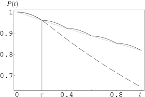
Figure 1: Evolution with frequent “pulsed” measurements: quantum Zeno effect. The dashed (full) line is the survival probability without (with) measurements. The gray line is the interpolating exponential (6).

3 From quantum Zeno to inverse quantum Zeno (“Heraclitus”)

Let us concentrate our attention on truly unstable systems, with a “natural” decay rate $\gamma$, given by the Fermi “golden” rule.[16] We ask: is it possible to find a finite time $\tau^{*}$ such that

$$\gamma_{\rm eff}(\tau^{*})=\gamma?$$ (9)

If such a time exists, then by performing measurements at time intervals $\tau^{*}$ the system decays according to its “natural” lifetime, as if no measurements were performed. The quantity $\tau^{*}$ is related to Schulman’s “jump” time.[24, 2]

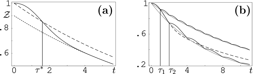
Figure 2: $\mathcal{Z}<1$. (a) Determination of $\tau^{*}$. (b) Quantum Zeno vs inverse quantum Zeno (“Heraclitus”) effect.

By Eqs. (9) and (7) one gets

$$P(\tau^{*})=e^{-\gamma\tau^{*}},$$ (10)

i.e., $\tau^{*}$ is the intersection between the curves $P(t)$ and $e^{-\gamma t}$. In the situation outlined in Figure 2(a) such a time $\tau^{*}$ exists: the full line is the survival probability and the dashed line the exponential $e^{-\gamma t}$ [the dotted line is the asymptotic exponential $\mathcal{Z}e^{-\gamma t}$, that will be defined in Eq. (31)]. The physical meaning of $\tau^{*}$ can be understood by looking at Figure 2(b), where the dashed line represents a typical behavior of the survival probability $P(t)$ when no measurement is performed: the short-time Zeno region is followed by an approximately exponential decay with a natural decay rate $\gamma$. When measurements are performed at time intervals $\tau$, we get the effective decay rate $\gamma_{\rm eff}(\tau)$. The full lines represent the survival probabilities and the dotted lines their exponential interpolations, according to (6). If $\tau=\tau_{1}<\tau^{*}$ one obtains QZE. Vice versa, if $\tau=\tau_{2}>\tau^{*}$, one obtains IZE. If $\tau=\tau^{*}$ one recovers the natural lifetime, according to (9): in this sense, amusingly, $\tau^{*}$ can be viewed as a transition time from Zeno (who argued that a sped arrow, if observed, does not move) to Heraclitus (who replied that everything flows). Heraclitus opposed Zeno and Parmenides’ (Zeno’s master) philosophical view.[22, 25]

Figure 3: $\mathcal{Z}>1$. The full line is the survival probability, the dashed line the renormalized exponential $e^{-\gamma t}$ and the dotted line the asymptotic exponential $\mathcal{Z}e^{-\gamma t}$. (a) If $P(t)$ and $e^{-\gamma t}$ do not intersect, a finite solution $\tau^{*}$ does not exist. (b) If $P(t)$ and $e^{-\gamma t}$ intersect, a finite solution $\tau^{*}$ exists. (In this case there are always at least two intersections.)

Sometimes (interestingly) $\tau^{*}$ does not exist: Eq. (9) may have no finite solutions. In such a case only QZE is possible and no IZE is attainable. This is in contrast with some recent claims,[26] according to which the inverse Zeno regime is easier to attain than the quantum Zeno one. We can get a qualitative idea of the meaning of these statements by looking at the survival probability of an unstable system for sufficiently long times[2]

$$P(t)=|\mathcal{A}(t)|^{2}\simeq\mathcal{Z}e^{-\gamma t},$$ (11)

where $\mathcal{Z}$, the intersection of the asymptotic exponential with the $t=0$ axis, is the square modulus of the residue of the pole of the propagator (wave function renormalization)[2, 22, 12] and will be defined in the next section [Eq. (31)].

A sufficient condition for the existence of a solution $\tau^{*}$ of Eq. (9) is that $\mathcal{Z}<1$. This is easily proved by graphical inspection. The case $\mathcal{Z}<1$ is shown in Figure 2(a): $P(t)$ with the property (11) and $e^{-\gamma t}$ must intersect. The other case, $\mathcal{Z}>1$, is shown in Figure 3: a solution may or may not exist, depending on the features of the model investigated. There are also situations (e.g., oscillatory systems, whose Poincaré time is finite) where $\gamma$ and $\mathcal{Z}$ cannot be defined.[22] The transition from Zeno to inverse Zeno is therefore a complex, model-dependent problem, that requires careful investigation. We shall come back to this issue in the following sections, where (11) will be derived for a particular field theoretical model.

4 The Lee Hamiltonian

Some of the most interesting Zeno phenomena, including the transition from a Zeno to a Heraclitus regime, arise in a quantum field theoretical framework.[8, 9, 10] We will now study the time evolution of a quantum system in greater detail, by making use of a quantum field theoretical techniques, and discuss the primary role played by the form factors of the interaction.

Consider a generic Hamiltonian $H$ and an initial normalized state $|{a}\rangle$. The total Hilbert space can always be decomposed into a direct sum $\mathcal{H}=\mathcal{H}_{a}\oplus\mathcal{H}_{d}$, with $\mathcal{H}_{a}=P_{a}\mathcal{H}$ and $\mathcal{H}_{d}=P_{d}\mathcal{H}$, where $P_{a}=|a\rangle\langle a|$ and $P_{d}=1-P_{a}$. Let us accordingly split the total Hamiltonian into a free and an interaction part

$$H=H_{0}+H_{\rm int},$$ (12)

where

$$H_{0}=P_{a}HP_{a}+P_{d}HP_{d},\qquad H_{\mathrm{int}}=P_{a}HP_{d}+P_{d}HP_{a}.$$ (13)

This decomposition can always be performed,[19] even in relativistic quantum field theory,[10] the only “problem” being that the decomposition itself depends on the initial state $|{a}\rangle$. Let $\{|{n}\rangle\}$ be the eigenbasis of $H_{0}$ in $\mathcal{H}_{d}$

$$\langle{a}|a\rangle=1,\quad\langle{a}|n\rangle=0,\quad\langle{n}|n^{\prime}\rangle=\delta_{nn^{\prime}},$$ (14)

$$H_{0}|{a}\rangle=\omega_{a}|{a}\rangle,\qquad H_{0}|{n}\rangle=\omega_{n}|{n}\rangle.$$ (15)

The interaction Hamiltonian $H_{\rm int}$ is completely off-diagonal and has nonvanishing matrix elements only between $\mathcal{H}_{a}$ and $\mathcal{H}_{d}$, namely

$$\langle{a}|H_{\rm int}|{n}\rangle=\langle{n}|H_{\rm int}|{a}\rangle^{*}=g_{n},\qquad\langle{a}|H_{\rm int}|{a}\rangle=\langle{n}|H_{\rm int}|{n^{\prime}}\rangle=0,\quad\forall n,n^{\prime}.$$ (16)

Equations (14)-(16) completely determine the free and interaction Hamiltonians in terms of the chosen basis. Indeed we get

$$H_{0}=\omega_{a}|{a}\rangle\langle{a}|+\sum_{n}\omega_{n}|{n}\rangle\langle{n}|,\qquad H_{\rm int}=\sum_{n}\left(g_{n}|{a}\rangle\langle{n}|+g_{n}^{*}|{n}\rangle\langle{a}|\right).$$ (17)

This is the Lee Hamiltonian[27] and was originally introduced as a solvable quantum field model for the study of the renormalization problem. The interaction of the normalizable state $|{a}\rangle$ with the states $|{n}\rangle$ (the formal sum in the above equation usually represents an integral over a continuum of states) is responsible for its decay and depends on the form factor $g_{n}$.

The Fourier-Laplace transform of the survival amplitude $\mathcal{A}(t)$ in (1) is the expectation value of the resolvent

$$G_{a}(E) = -i\int_{0}^{\infty}dt\;e^{iEt}\mathcal{A}(t)=\langle{a}|\frac{1}{E-H}|{a}\rangle,$$

$$\mathcal{A}(t) = \frac{i}{2\pi}\int_{\rm B}dE\;e^{-iEt}G_{a}(E),$$ (18)

the Bromwich path B being a horizontal line $\mathrm{Im}E=$constant$>0$ in the half plane of convergence of the Fourier-Laplace transform (upper half plane). By performing Dyson’s resummation, the propagator reads

$$G_{a}(E)=\frac{1}{E-\omega_{a}-\Sigma_{a}(E)},$$ (19)

where the self-energy function

$$\Sigma_{a}(E)=\sum_{n}\frac{\left|\langle{a}|H_{\rm int}|{n}\rangle\right|^{2}}{E-\omega_{n}}=\int d\omega\;\frac{\kappa_{a}(\omega)}{E-\omega}$$ (20)

consists only of a second order contribution and is related to the form factor $g_{n}$ by the equation

$$\kappa_{a}(E)=\sum_{n}\left|\langle{a}|H_{\rm int}|{n}\rangle\right|^{2}\delta(E-\omega_{n})=\sum_{n}|g_{n}|^{2}\delta(E-\omega_{n}).$$ (21)

A comment is now in order. If one is only interested in the survival amplitude [or, equivalently, in the expression of the propagator (19)] and not in the details of the interactions $g_{n}$ between $|{a}\rangle$ and different states $|{n}\rangle$ with the same energy $\omega_{n}=\omega$, one can simply replace this set of states with a single, representative state $|{\omega}\rangle$, by replacing the Hamiltonian (17) with the following equivalent one

$$H=H_{0}+H_{\rm int}=\omega_{a}|{a}\rangle\langle{a}|+\int d\omega\;\omega|{\omega}\rangle\langle{\omega}|+\int d\omega\;g(\omega)(|{a}\rangle\langle{\omega}|+|{\omega}\rangle\langle{a}|),$$ (22)

where the form factor $g(\omega)=\sqrt{\kappa_{a}(\omega)}$ and

$$|{a}\rangle\langle{a}|+\int d\omega\;|{\omega}\rangle\langle{\omega}|=1.$$ (23)

In terms of the Hamiltonian (22) the self-energy function simply reads

$$\Sigma_{a}(E)=\int d\omega\;\frac{\left|\langle{a}|H_{\rm int}|{\omega}\rangle\right|^{2}}{E-\omega}=\int d\omega\;\frac{g^{2}(\omega)}{E-\omega}.$$ (24)

5 Unstable systems

We consider now the case of an unstable system. The initial state has energy $\omega_{a}>\omega_{g}$ ($\omega_{g}$ being the lower bound of the continuous spectrum of the Hamiltonian $H$) and is therefore embedded in the continuous spectrum of $H$. If $-\Sigma_{a}(\omega_{g})<\omega_{a}$ (which happens for sufficiently smooth form factors and small coupling), the resolvent is analytic in the whole complex plane cut along the real axis (continuous spectrum of $H$). On the other hand, there exists a pole $E_{\mathrm{pole}}$ located just below the branch cut in the second Riemann sheet, solution of the equation

$$E_{\rm pole}-\omega_{a}-\Sigma_{a{\rm II}}(E_{\rm pole})=0,$$ (25)

$\Sigma_{a{\rm II}}$ being the determination of the self-energy function in the second sheet. The pole has a real and imaginary part

$$E_{\rm pole}=\omega_{a}+\delta\omega_{a}-i\gamma/2$$ (26)

given by

$$\delta\omega_{a} = \mathrm{Re}\Sigma_{a{\rm II}}(E_{\rm pole})\simeq\mathrm{Re}\Sigma_{a}(\omega_{a}+i0^{+})={\rm P}\!\!\int d\omega\frac{g^{2}(\omega)}{\omega_{a}-\omega},$$ (27)

$$\gamma = -2\mathrm{Im}\Sigma_{a{\rm II}}(E_{\rm pole})\simeq-2\mathrm{Im}\Sigma_{a}(\omega_{a}+i0^{+})=2\pi g^{2}(\omega_{a}),$$ (28)

up to fourth order in the coupling constant. One recognizes the second-order energy shift $\delta\omega_{a}$ and the celebrated Fermi “golden” rule $\gamma$.[16] The survival amplitude has the general form

$$\mathcal{A}(t)=\mathcal{A}_{\rm pole}(t)+\mathcal{A}_{\rm cut}(t),$$ (29)

where

$$\mathcal{A}_{\rm pole}(t)=e^{-i(\omega_{a}+\delta\omega_{a})t-\gamma t/2}/[1-\Sigma^{\prime}_{a{\rm II}}(E_{\rm pole})],$$ (30)

$\mathcal{A}_{\rm cut}$ being the branch-cut contribution. At intermediate times, the pole contribution dominates the evolution and

$$P(t)\simeq|\mathcal{A}_{\rm pole}(t)|^{2}=\mathcal{Z}e^{-\gamma t},\qquad\mathcal{Z}=\left|1-\Sigma^{\prime}_{a{\rm II}}(E_{\rm pole})\right|^{-2},$$ (31)

where $\mathcal{Z}$, the intersection of the asymptotic exponential with the $t=0$ axis, is the wave function renormalization. We have found (11) and explicitly determined $\mathcal{Z}$.

Notice that, in order to obtain a purely exponential decay, one neglects all branch cut and/or other contributions from distant poles and considers only the contribution of the dominant pole. In other words, one does not look at the rich analytical structure of the propagator and retains only its dominant polar singularity. In this case the self-energy function becomes a constant (equal to its value at the pole), namely

$$G_{a}(E)\longrightarrow G_{a}^{\rm WW}(E)=\frac{1}{E-\omega_{a}-\Sigma_{a\rm II}(E_{\rm pole})}=\frac{1}{E-E_{\rm pole}},$$ (32)

where in the last equality we used the pole equation (25). This is the celebrated Weisskopf-Wigner approximation[15] and yields a purely exponential behavior, $\mathcal{A}(t)=\exp(-iE_{\rm pole}t)$, without short- and long-time corrections.

As is well known, the exponential law is corrected by the cut contribution, which is responsible for a quadratic behavior at short times and a power law at long times. In particular, at short times, by plugging (19) into (18) and changing the integration variable $\eta=Et$, Eq. (18) becomes

$$\mathcal{A}(t)={i\over 2\pi}\int_{B}d\eta\;\frac{e^{-i\eta}}{\eta-\omega_{a}t-t\;\Sigma_{a}(\eta/t)}.$$ (33)

The self-energy function (24) has the following behavior at large energies

$$\Sigma_{a}\left(E\right)\sim\frac{1}{E}\int d\omega g^{2}(\omega)=\frac{1}{E}\langle{a}|H_{\mathrm{int}}^{2}|{a}\rangle=\frac{1}{\tau_{\mathrm{Z}}^{2}E},\qquad E\to\infty$$ (34)

where we used Eq. (4) (and assumed the existence of the second moment of the Hamiltonian $H_{\mathrm{int}}$). Therefore, the survival amplitude at small times has the asymptotic expansion

$$\mathcal{A}(t)\sim\frac{i}{2\pi}\int_{B}d\eta\,\frac{\eta e^{-i\eta}}{\eta^{2}-\omega_{a}t\eta-t^{2}/\tau_{\rm Z}^{2}}=\frac{i}{2\pi}\int_{B}d\eta\,\frac{\eta e^{-i\eta}}{(\eta-t\eta_{1})(\eta-t\eta_{2})},$$ (35)

where

$$\eta_{1,2}=\frac{\omega_{a}}{2}\pm\sqrt{\left(\frac{\omega_{a}}{2}\right)^{2}+\frac{1}{\tau_{\rm Z}^{2}}}.$$ (36)

By closing the Bromwich path in Eq. (35) with a large semicircle in the lower half plane, the integral reduces to the sum of the residues at the real poles $t\eta_{1,2}$ and the survival probability at small times reads

$$P(t)=|\mathcal{A}(t)|^{2}\sim\frac{\eta_{1}^{2}+\eta_{2}^{2}-2\eta_{1}\eta_{2}\cos[t(\eta_{1}-\eta_{2})]}{(\eta_{1}-\eta_{2})^{2}}\sim 1+\eta_{1}\eta_{2}t^{2}=1-\frac{t^{2}}{\tau_{\rm Z}^{2}},\ \$$ (37)

in agreement with the expansion (2). Notice that at short times the behavior is governed by two “effective” poles which replace the global contribution of the cut and the pole on the second sheet. We will come back to this important point in the following sections.

6 Two-pole model and two-pole reduction

We consider now a particular solvable model: let the form factor in (22) be Lorentzian

$$g(\omega)=\frac{\lambda}{\sqrt{\pi}}\sqrt{\frac{\Lambda}{\omega^{2}+\Lambda^{2}}}.$$ (38)

This describes, for instance, an atom-field coupling in a cavity with high finesse mirrors.[28] (Notice that the Hamiltonian in this case is not lower bounded and we expect no deviations from exponential behavior at very large times.[29]) In this case one easily obtains (for $\mathrm{Im}E>0$)

$$\Sigma_{a}(E)=\frac{\lambda^{2}}{E+i\Lambda},$$ (39)

whence the propagator

$$G_{a}(E)=\frac{E+i\Lambda}{(E-\omega_{a})(E+i\Lambda)-\lambda^{2}}$$ (40)

has two poles in the lower half energy plane (see Fig. 4). Their values are

$$E_{1}=\omega_{a}+\delta\omega_{a}-i\frac{\gamma}{2},\quad E_{2}=-\delta\omega_{a}-i\left(\Lambda-\frac{\gamma}{2}\right),$$ (41)

where

$$\left\{\begin{array}[]{c}\delta\omega_{a}=-\frac{\omega_{a}}{2}+\frac{\omega_{a}}{2}\sqrt{\frac{\sqrt{\upsilon^{4}+4\omega_{a}^{2}\Lambda^{2}}+\upsilon^{2}}{2\omega_{a}^{2}}}\\ \\ \gamma=\Lambda-\sqrt{\frac{\sqrt{\upsilon^{4}+4\omega_{a}^{2}\Lambda^{2}}-\upsilon^{2}}{2}}\end{array}\right.,\quad\mbox{with}\quad\upsilon^{2}=\omega_{a}^{2}+4\lambda^{2}-\Lambda^{2}.$$ (42)

(Notice that $\upsilon^{2}$ can be negative.)

Figure 4: (a) Form factor $g^{2}(\omega)$ and initial state energy $\omega_{a}$. (b) Poles of the propagator in the complex $E$-plane.

The propagator and the survival amplitude read

$$G_{a}(E) = \frac{E_{1}+i\Lambda}{E_{1}-E_{2}}\frac{1}{E-E_{1}}-\frac{E_{2}+i\Lambda}{E_{1}-E_{2}}\frac{1}{E-E_{2}}$$ (43)

$$= \frac{1-\mathcal{R}}{E-(\omega_{a}+\delta\omega_{a})+i\gamma/2}+\frac{\mathcal{R}}{E+\delta\omega_{a}+i(\Lambda-\gamma/2)}$$

and

$$\mathcal{A}(t)=(1-\mathcal{R})e^{-i(\omega_{a}+\delta\omega_{a})t}e^{-\gamma t/2}+\mathcal{R}e^{i\delta\omega_{a}t}e^{-(\Lambda-\gamma/2)t},$$ (44)

respectively, where

$$1-\mathcal{R}=\mbox{Res}[G_{a}(E_{1})]=\frac{1}{1-\Sigma_{a}^{\prime}(E_{1})}=\frac{\omega_{a}+\delta\omega_{a}+i(\Lambda-\gamma/2)}{\omega_{a}+2\delta\omega_{a}+i(\Lambda-\gamma)}$$ (45)

is the residue of the pole $E_{1}$ of the propagator. The survival probability reads

$$P(t)=|\mathcal{A}(t)|^{2} = \mathcal{Z}\exp(-\gamma t)+2\mbox{Re}[\mathcal{R}^{*}(1-\mathcal{R})e^{-i(\omega_{a}+2\delta\omega_{a})t}]\exp(-\Lambda t)$$ (46)

$$+|\mathcal{R}|^{2}\exp[-(2\Lambda-\gamma)t],$$

where $\mathcal{Z}=|1-\mathcal{R}|^{2}$ is the wave function renormalization

$${\cal Z}=\frac{(\omega_{a}+\delta\omega_{a})^{2}+(\Lambda-\gamma/2)^{2}}{(\omega_{a}+2\delta\omega_{a})^{2}+(\Lambda-\gamma)^{2}}\ .$$ (47)

All the above formulas are exact. We now analyze some interesting limits of the model investigated.

6.1 Small coupling

In the weak coupling limit $\lambda\ll\omega_{a},\Lambda$, one obtains from Eq. (42)

$$\delta\omega_{a} = \frac{\lambda^{2}}{\omega_{a}^{2}+\Lambda^{2}}\omega_{a}+\mathrm{O}(\lambda^{4})={\rm P}\!\!\int d\omega\frac{g^{2}(\omega)}{\omega_{a}-\omega}+\mathrm{O}(\lambda^{4}),$$

$$\gamma = 2\Lambda\frac{\lambda^{2}}{\omega_{a}^{2}+\Lambda^{2}}+\mathrm{O}(\lambda^{4})=2\pi g^{2}(\omega_{a})+\mathrm{O}(\lambda^{4}).$$ (48)

Notice that the latter formula is the Fermi Golden Rule and $E_{1}$ in (41) is the “dominant” pole. Indeed, the second exponential in Eq. (44) is damped very quickly, on a time scale $\Lambda^{-1}$ much faster than $\gamma^{-1}$, whence, after a short initial quadratic (Zeno) region of duration $\Lambda^{-1}$, the decay becomes purely exponential with decay rate $\gamma$. Notice that the corrections are of order $\lambda^{2}$

$$\mathcal{R}=\frac{\lambda^{2}}{\omega_{a}^{2}+\Lambda^{2}}\frac{\omega_{a}-i\Lambda}{\omega_{a}+i\Lambda}+\mathrm{O}(\lambda^{4})$$ (49)

and the Zeno time is $\tau_{\rm Z}=\lambda^{-1}\gg\Lambda^{-1}$, i.e. the initial quadratic (Zeno) region is much shorter than the Zeno time: in general, the Zeno time does not yield a correct estimate of the duration of the Zeno region.[9, 22, 30] (Beware of many erroneous claims in the literature!) The approximation $P(t)\simeq 1-t^{2}/\tau_{\rm Z}^{2}$ holds for times $t<\Lambda^{-1}\ll\tau_{\rm Z}$.

6.2 Large bandwidth

In the limit of large bandwidth $\Lambda\gg\omega_{a},\lambda$, from Eq. (42) one gets $\gamma=2\lambda^{2}/\Lambda+\mathrm{O}(\Lambda^{-2})$ and in order to have a non trivial result with a finite decay rate, we let

$$\Lambda\to\infty,\quad\lambda\to\infty,\qquad\mbox{with}\quad\frac{\lambda^{2}}{\Lambda}=\frac{\gamma}{2}=\mbox{const}.$$ (50)

In this limit the continuum has a flat band, $g(\omega)=\sqrt{\gamma/2\pi}=$const, and we expect to recover a purely exponential decay. Indeed, in this case one gets $\mathcal{R}=0$ and $\delta\omega_{a}=0$, whence

$$G_{a}(E)=\frac{1}{E-\omega_{a}+i\gamma/2},$$ (51)

so that the survival amplitude and probability read

$$\mathcal{A}(t)=\exp\left(-i\omega_{a}t-\frac{\gamma}{2}t\right)\quad\mbox{and}\quad P(t)=\exp(-\gamma t).$$ (52)

In this case the propagator (51) has only a simple pole and the survival probability (52) is purely exponential.

6.3 Narrow bandwidth

In the limit of narrow bandwidth $\Lambda\ll\omega_{a},\lambda$, the form factor becomes

$$g^{2}(\omega)=\lambda^{2}\delta(\omega)$$ (53)

and the continuum is “concentrated” in $\omega=0$. Therefore the continuum as a whole behaves as another discrete level and one obtains Rabi oscillations between the initial state $|{a}\rangle$ in (22) and this “collective” level (of energy $\omega=0$). In fact one gets

$$\gamma=0,\quad\delta\omega_{a}=-\frac{\omega_{a}}{2}+\Omega,\quad\mathcal{R}=\frac{1}{2}\left(1-\frac{\omega_{a}}{2\Omega}\right),$$ (54)

where

$$\Omega=\sqrt{\lambda^{2}+\frac{\omega_{a}^{2}}{4}}$$ (55)

is the usual Rabi frequency of a two-level system with energy difference $\omega_{a}(=\omega_{a}-0)$ and coupling $\lambda$. By (54) the survival amplitude and probability read

$$\mathcal{A}(t) = \frac{1}{2}\left(1+\frac{\omega_{a}}{2\Omega}\right)e^{-i(\omega_{a}+\Omega)t}+\frac{1}{2}\left(1-\frac{\omega_{a}}{2\Omega}\right)e^{-i(\omega_{a}-\Omega)t},$$

$$P(t) = 1-\frac{\lambda^{2}}{\Omega^{2}}\sin^{2}\left(\frac{\Omega t}{2}\right).$$ (56)

If $\omega_{a}=0$, the survival probability (56) oscillates between $1$ and $0$. On the other hand, if $\omega_{a}\neq 0$ the initial state never “decays” completely.

Incidentally, notice that the Zeno time is still $\tau_{\rm Z}=\lambda^{-1}$ and yields now a good estimate of the duration of the Zeno region. This is, so to say, a “coincidence” due to the oscillatory features of the system.

6.4 Strong coupling

Another interesting case is that of strong coupling, $\lambda\simeq\Lambda$. This is a typical case in which the strong coupling provokes violent oscillations before the system reaches the asymptotic regime. In the limit $\lambda\gg\Lambda,\omega_{a}$, we get

$$\delta\omega_{a}=\lambda-\frac{\omega_{a}}{2}+\mathrm{O}(\lambda^{-1}),\quad\gamma=-i\frac{\Lambda}{2}+\mathrm{O}(\lambda^{-1}),\quad\mathcal{R}=\frac{1}{2}-\frac{\omega_{a}+i\Lambda}{4\lambda}+\mathrm{O}(\lambda^{-3}),$$ (57)

whence the survival amplitude reads

$$\mathcal{A}(t)\simeq\exp\left(-i\frac{\omega_{a}}{2}t-\frac{\Lambda}{2}t\right)\left[\left(\frac{1}{2}+\frac{\omega_{a}+i\Lambda}{4\lambda}\right)e^{-i\lambda t}+\left(\frac{1}{2}-\frac{\omega_{a}+i\Lambda}{4\lambda}\right)e^{i\lambda t}\right],$$ (58)

which yields fast oscillations of frequency $\lambda$ damped at a rate $\Lambda\ll\lambda$.

6.5 Two-pole reduction

We now show that the two-pole model introduced in this section is the first improvement, after the Weisskopf-Wigner pole, in the approximation of a generic quantum field model. First note that, according to the Weisskopf-Wigner approximation (32), an exponential decay is obtained by considering a constant self-energy function $\Sigma_{a}=-i\gamma/2$, i.e. a resolvent with a single pole with negative imaginary part ($E_{1}$ in Figure 4). On the other hand, as we noted in Sec. 5, the initial quadratic behavior of the survival amplitude is governed by two effective poles of the resolvent, which ultimately derive from the behavior (34) of the self-energy function at infinity

$$\Sigma_{a}(E)\sim\frac{1}{\tau_{\rm Z}^{2}E},\qquad\mbox{for}\quad E\to\infty.$$ (59)

If one wants to capture this short-time behavior while keeping the exponential law at later times, and is not interested in the long-time power-law deviations, one can proceed in the following way. The requirement for having an exponential decay, with decay rate $\gamma$ for $t\to\infty$, translates into the behavior of the self-energy function for $E\to 0$, namely in the requirement of having a Weisskopf-Wigner constant self-energy function with negative imaginary part

$$\Sigma_{a}(0)=-ib.\quad(b>0)$$ (60)

The simplest form of the self-energy function satisfying both requirements (59) and (60) is

$$\Sigma_{a}(E)=\frac{1}{\tau_{\rm Z}^{2}E+i/b}=\frac{1/\tau_{\rm Z}^{2}}{E+i/b\tau_{Z}^{2}}$$ (61)

By letting $\tau_{\rm Z}=1/\lambda$ and $1/b\tau_{Z}^{2}=\Lambda$, this becomes exactly the self-energy function of the two-pole model (39). Therefore the two-pole model is the simplest approximation which yields the short time quadratic behavior together with the long time exponential one.

We call the technique outlined in this subsection “two-pole reduction.” It is useful if one wants to get a first idea of the temporal behavior of a quantum field, keeping information on the lifetime (Fermi golden rule), but also on the short-time Zeno region.

Note that the process outlined above can be iterated to find better approximations of the real self-energy function $\Sigma_{a}(E)$ by adding other poles and/or zeros. But notice also that this approach does not yield the inverse power-law tail. Indeed the latter is essentially due to the nonanalytic behavior of the self-energy function at the branching point, a feature that cannot be captured by an olomorphic function.

7 Modification of the Lee Hamiltonian

We now introduce an interesting modification of the Lee Hamiltonian (22), which enables us to look at the Zeno region from a different perspective. The Hamiltonian (22) describes the decay of a discrete state $|{a}\rangle$ into a continuum of states $|{\omega}\rangle$ with a given form factor $g(\omega)$. According to Eqs. (4) and (22), the Zeno time is related to the integral of the squared form factor by the simple relation

$$\frac{1}{\tau_{\rm Z}^{2}}=\int d\omega\;g^{2}(\omega).$$ (62)

On the other hand, for a two-level system $\{|{a}\rangle,|{b}\rangle\}$ with Hamiltonian

$$H=\lambda(|{a}\rangle\langle{b}|+|{b}\rangle\langle{a}|),\quad\tau_{\rm Z}=1/\lambda$$ (63)

the Zeno time $\tau_{\rm Z}$ is just the inverse off-diagonal element $\lambda$ of the Hamiltonian [and, of course, this is in agreement with Eq. (62), as shown by Eq. (53)]. One has therefore a simple system in which the Zeno time is manifest in the Hamiltonian itself. We seek now an equivalent decay model, that shares with the two-level model this nice property. To this end, let us add a new “intermediate” discrete state $|{b}\rangle$ to the Lee model. Consider then the Rabi oscillation $\lambda$ of the two-level system $|{a}\rangle$, $|{b}\rangle$ and let the initial state $|{a}\rangle$ decay only through state $|{b}\rangle$, i.e. couple $|{b}\rangle$ to a continuum with form factor $g_{b}(\omega)$. In other words, the Hamiltonian (22) is substituted by the following one

$$H = \omega_{a}|{a}\rangle\langle{a}|+\omega_{b}|{b}\rangle\langle{b}|+\int d\omega\;\omega|{\omega}\rangle\langle{\omega}|$$ (64)

$$+\lambda\left(|{a}\rangle\langle{b}|+|{b}\rangle\langle{a}|\right)+\int d\omega\;g_{b}(\omega)(|{b}\rangle\langle{\omega}|+|{\omega}\rangle\langle{b}|).$$

We require that this Hamiltonian is equivalent to the original one in describing the decay of the initial state $|{a}\rangle$. To this end, notice that the part of Hamiltonian describing the decay of state $|{b}\rangle$ (and neglecting the coupling with $|{a}\rangle$) is just a Lee Hamiltonian and gives

$$G_{b}(E)=\frac{1}{E-\omega_{b}-\Sigma_{b}(E)},\qquad\Sigma_{b}(E)=\int d\omega\;\frac{g_{b}^{2}(\omega)}{E-\omega}.$$ (65)

On the other hand, state $|{a}\rangle$ couples only to state $|{b}\rangle$ with a coupling $\lambda$. Therefore the evolution of state $|{a}\rangle$ is just a Rabi oscillation between state $|{b}\rangle$ dressed by the continuum $|{\omega}\rangle$ and state $|{a}\rangle$, namely

$$G_{a}=G_{a}^{0}+G_{a}^{0}\lambda G_{b}\lambda G_{a}\ ,$$ (66)

whence

$$G_{a}(E)=\frac{1}{E-\omega_{a}-\lambda^{2}G_{b}(E)}\ .$$ (67)

Therefore, in the modified model, the self-energy function of the initial state $|{a}\rangle$ is nothing but the coupling $\lambda^{2}$ times the dressed propagator $G_{b}(E)$

$$\Sigma_{a}(E)=\lambda^{2}G_{b}(E)=\frac{\lambda^{2}}{E-\omega_{b}-\Sigma_{b}(E)}.$$ (68)

Equation (68) is the equivalence relation sought. One has to choose the auxiliary form factor $g_{b}(\omega)$ in Eq. (64) as a function of the original one $g(\omega)$, in order to satisfy this relation and get an equivalent description of the decay. Our interest in this equivalence is due to the asymptotic behavior of formula (68)

$$\Sigma_{a}(E)\sim\frac{\lambda^{2}}{E}=\frac{1}{\tau_{\rm Z}^{2}E},\qquad\mbox{for}\quad E\to\infty\ ,$$ (69)

which displays the relation between the coupling $\lambda$ and the Zeno time $\tau_{\rm Z}$. Thus the Hamiltonian (64) explicitly reads

$$H = \omega_{a}|{a}\rangle\langle{a}|+\omega_{b}|{b}\rangle\langle{b}|+\frac{1}{\tau_{\rm Z}}\left(|{a}\rangle\langle{b}|+|{b}\rangle\langle{a}|\right)$$ (70)

$$+\int d\omega\;\omega|{\omega}\rangle\langle{\omega}|+\int d\omega\;g_{b}(\omega)(|{b}\rangle\langle{\omega}|+|{\omega}\rangle\langle{b}|).$$

In the equivalent model, therefore, the initial quadratic behavior is singled out from the remaining part of the decay: the Zeno region, i.e. the first oscillation, is nothing but the initial unperturbed Rabi oscillation between states $|{a}\rangle$ and $|{b}\rangle$ (which initially “represents” the original continuum as a whole). After the initial stage of the decay, the coupling $g_{b}(\omega)$ between $|{b}\rangle$ and $|{\omega}\rangle$ (namely the details of the original continuum) comes into play and modifies the initial Rabi oscillation with its characteristic time scale. This explains from a different perspective the difference, already stressed in previous sections, between the Zeno time and the duration of the initial quadratic region.

Figure 5: The decay of state $|{a}\rangle$ into a Lorentzian continuum $|{\omega}\rangle$ (a) is exactly equivalent to a Rabi coupling of $|{a}\rangle$ with a state $|{b}\rangle$ that in turn exponentially decays into a flat continuum $|{\omega}\rangle$ (b).

As an example, we recover the self-energy function (39) of the two-pole model, by requiring that $\Sigma_{b}$ be constant

$$\Sigma_{b}(E)=-\omega_{b}-i\Lambda\ ,$$ (71)

which implies

$$g_{b}(\omega)=\sqrt{\Lambda/\pi}\qquad\mbox{and}\quad\omega_{b}=0.$$ (72)

In other words, the auxiliary state $|{b}\rangle$ is placed at the mean energy of the original continuum $g(\omega)$ and decays into a flat-band continuum with decay rate $\gamma_{b}=2\Lambda$: the decay into a Lorentzian continuum [Fig. 5(a)] is exactly equivalent to a Rabi coupling with a level that in turn exponentially decays into a flat continuum [Fig. 5(b)]:

$$H = \omega_{a}|{a}\rangle\langle{a}|+\frac{1}{\tau_{\mathrm{Z}}}\left(|{a}\rangle\langle{b}|+|{b}\rangle\langle{a}|\right)+\int d\omega\;\omega|{\omega}\rangle\langle{\omega}|$$ (73)

$$+\sqrt{\frac{\Lambda}{\pi}}\int d\omega\;(|{b}\rangle\langle{\omega}|+|{\omega}\rangle\langle{b}|).$$

Moreover, if one restricts one’s attention to the subspace spanned by $\{|{a}\rangle,|{b}\rangle\}$, it is easy to show[22] that this Hermitian Hamiltonian reduces to the effective non-Hermitian one

$$H = \omega_{a}|{a}\rangle\langle{a}|+\lambda\left(|{a}\rangle\langle{b}|+|{b}\rangle\langle{a}|\right)-i\Lambda|{b}\rangle\langle{b}|$$ (78)

$$= \left(\begin{array}[]{cc}\omega_{a}&\lambda\\ \lambda&-i\Lambda\end{array}\right)=\left(\begin{array}[]{cc}\omega_{a}&\tau_{\mathrm{Z}}^{-1}\\ \tau_{\mathrm{Z}}^{-1}&-i\left(\frac{\gamma}{2}+\frac{2}{\tau_{\mathrm{Z}}^{2}\gamma}\frac{1}{1+4\delta\omega_{a}^{2}/\gamma^{2}}\right)\end{array}\right)$$

Therefore, if one is interested only in the decay of the initial state $|{a}\rangle$, the study of the two-pole model reduces to the study of this simple non-Hermitian 2-dimensional matrix. One can reexamine all the results of previous sections, just by looking at this matrix. We will not elaborate on this here.

A final comment is now in order. One can draw a clear picture of the two-pole reduction, discussed in the previous section, just by looking at the construction of the equivalent model. The first approximation of a real decay, the Weisskopf-Wigner approximation, is represented by the simple exponential decay of level $|{b}\rangle$ with its time scale $\gamma_{b}^{-1}$. The two-pole approximation superimposes an oscillating dynamics with time scale $\lambda^{-1}$ to the latter, yielding the initial Zeno region. By complicating the model with the addition of other dynamical elements with their characteristic scales, one can construct a better approximation of the real decay law.

8 Zeno–Heraclitus transition

We will now study the Zeno–inverse Zeno transition in greater detail, by making use of a quantum field theoretical framework, and discuss the primary role played by the form factors of the interaction. The reader should refer to the discussion of Secs. 2-3, where we introduced the effective decay rate

$$\gamma_{\rm eff}(\tau)\equiv-\frac{1}{\tau}\log P(\tau)=-\frac{2}{\tau}\log|\mathcal{A}(\tau)|=-\frac{2}{\tau}\mathrm{Re}\Big{[}\log\mathcal{A}(\tau)\Big{]},$$ (79)

which is a linear function of $\tau$ for sufficiently small values of $\tau$ (inside the Zeno region)

$$\gamma_{\rm eff}(\tau)\sim\frac{\tau}{\tau_{\rm Z}^{2}},\qquad\mbox{for}\quad\tau\lesssim 1/\Lambda,$$ (80)

and becomes, with excellent approximation, a constant equal to the natural decay rate at intermediate times

$$\gamma_{\rm eff}(\tau)\simeq\gamma\qquad\mbox{for}\quad\tau\gg 1/\Lambda.$$ (81)

The transition between Zeno and Heraclitus occurs at the geometrical intersection $\tau^{*}$ between the curves $P(t)$ and $e^{-\gamma t}$, solution of the equation

$$\gamma_{\rm eff}(\tau^{*})=\gamma\ ,$$ (82)

as shown in Fig. 2.

Let us corroborate these general findings by considering for example the two-pole model studied in detail in Sec. 6, whose survival amplitude is given by Eq. (44)

$$\mathcal{A}(t) = \frac{\omega_{a}+\delta\omega_{a}+i(\Lambda-\gamma/2)}{\omega_{a}+2\delta\omega_{a}+i(\Lambda-\gamma)}e^{-i(\omega_{a}+\delta\omega_{a})t}e^{-\gamma t/2}$$ (83)

$$+\frac{\delta\omega_{a}-i\gamma/2}{\omega_{a}+2\delta\omega_{a}+i(\Lambda-\gamma)}e^{i\delta\omega_{a}t}e^{-(\Lambda-\gamma/2)t},$$

with $\delta\omega_{a}$ and $\gamma$ given by Eq. (42). By plugging (83) into (79) one obtains the effective decay rate, whose behavior is displayed in Fig. 6 for different values of the ratio $|\omega_{a}|/\Lambda$. These curves show that for large values of $|\omega_{a}|$ (in units $\Lambda$) there is indeed a transition from a Zeno to an inverse Zeno (Heraclitus) behavior: such a transition occurs at $\tau=\tau^{*}$, solution of Eq. (82). However, for small values of $|\omega_{a}|$, such a solution ceases to exist.

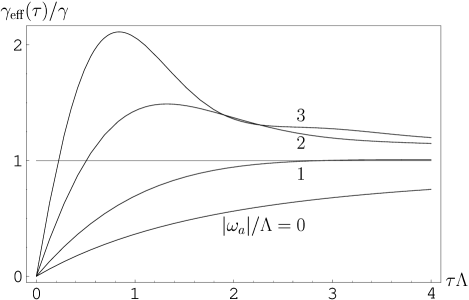
Figure 6: Effective decay rate $\gamma_{\rm eff}(\tau)$ for the two-pole model (83), for $\lambda=0.1$ and different values of the ratio $|\omega_{a}|/\Lambda$ (indicated). The horizontal line shows the “natural” decay rate $\gamma$: its intersection with $\gamma_{\rm eff}(\tau)$ yields the solution $\tau^{*}$ of Eq. (82). The asymptotic value of all curves is $\gamma$, as expected. A Zeno (inverse Zeno) effect is obtained for $\tau<\tau^{*}$ ($\tau>\tau^{*}$). Notice the presence of a linear region for small values of $\tau$ and observe that $\tau^{*}$ does not belong to such linear region as the ratio $|\omega_{a}|/\Lambda$ decreases. Above a certain threshold, given by Eq. (85) in the weak coupling limit of the model (and in general by the condition $\mathcal{Z}=1$), Eq. (82) has no finite solutions: only a Zeno effect is realizable in such a case.

The determination of the critical value of $|\omega_{a}|$ for which the Zeno–inverse Zeno transition ceases to take place discloses an interesting aspect of this issue. The problem can be discussed in general, but for the sake of simplicity we consider the weak coupling limit (small $\lambda$) considered in Eqs. (48)-(49). According to the geometrical theorem proved in Sec. 3, a sufficient condition for the system to exhibit an Zeno–inverse Zeno transition is that the wave function renormalization $\mathcal{Z}<1$. In our case, by making use of Eq. (49), this condition reads

$$\mathcal{Z} = |1-\mathcal{R}|^{2}=1-2\frac{\lambda^{2}}{\omega_{a}^{2}+\Lambda^{2}}\mbox{Re}\left[\frac{\omega_{0}-i\Lambda}{\omega_{a}+i\Lambda}\right]+\mathrm{O}(\lambda^{4})$$ (84)

$$= 1-2\frac{\lambda^{2}}{\omega_{a}^{2}+\Lambda^{2}}\frac{\omega_{a}^{2}-\Lambda^{2}}{\omega_{a}^{2}+\Lambda^{2}}+\mathrm{O}(\lambda^{4})<1,$$

namely

$$\omega_{a}^{2}>\Lambda^{2}+\mathrm{O}(\lambda^{2}).$$ (85)

The meaning of this relation is the following: a sufficient condition to obtain a Zeno–inverse Zeno transition is that the energy of the decaying state be placed asymmetrically with respect to the peak of the form factor (bandwidth) (see Fig. 4). If, on the other hand, $\omega_{a}\simeq 0$ (center of the bandwidth), no transition time $\tau^{*}$ exists (see Fig. 6) and only a QZE is possible: this is the case analyzed in Fig. 3(a).

There is more: Equation (83) yields a time scale. Indeed, from the definitions of the quantities in (42) one gets $\gamma/2<\Lambda-\gamma/2$, so that the second exponential in (83) vanishes more quickly than the first one. (The two time scales become comparable only in the strong coupling regime: $\gamma\to\Lambda$ as $\lambda\to\infty$.) If the coupling is weak, since $\gamma=\mbox{O}(\lambda^{2})$, the second term is very rapidly damped so that, after a short initial quadratic region of duration $\Lambda^{-1}$, the decay becomes purely exponential with decay rate $\gamma$. For $\tau\lesssim 1/\Lambda$ (which is, by definition, the duration of the quadratic Zeno region), we can use the linear approximation (80). When it applies up to the intersection (i.e., $|\omega_{a}|\gg\Lambda$) one gets

$$\tau^{*}\simeq\gamma\tau_{\rm Z}^{2}.$$ (86)

When $\omega_{a}$ gets closer to the peak of the form factor, the linear approximation does not hold and the r.h.s. of the above expression yields only a lower bound to the transition time $\tau^{*}$. In this case the solution $\tau^{*}$ of Eq. (82) becomes larger than the approximation (86), eventually going to infinity when condition (85) is no longer valid. In such a case, only a QZE is possible and no IZE is attainable. This is in contrast with recent claims.[26]

The conclusions obtained for the two-pole model (83) are of general validity. In general, in the Lee Hamiltonian (22), for any $g(\omega)$, we assume that $\omega_{a}>\omega_{g}$ (the lower bound of the continuous spectrum), in order to get an unstable system. The matrix elements of the interaction Hamiltonian depend of course on the physical model considered. However, for physically relevant situations, the interaction smoothly vanishes for small values of $\omega-\omega_{g}$ and quickly drops to zero for $\omega>\Lambda$, a frequency cutoff related to the size of the decaying system and the characteristics of the environment. This is true both for cavities, as well as for typical EM decay processes in vacuum, where the bandwidth $\Lambda\simeq 10^{14}-10^{18}$s^-1 is given by an inverse characteristic length[12, 22] (say, of the order of Bohr radius) and is much larger than the natural decay rate $\gamma\simeq 10^{7}-10^{9}$s^-1.

For roughly bell-shaped form factors all the conclusions drawn for the Lorentzian model remain valid. The main role is played by the ratio $\omega_{ag}/\Lambda$, where $\omega_{ag}=\omega_{a}-\omega_{g}$ is the available energy. In general, the asymmetry condition $\omega_{ag}<\Lambda$ is satisfied if the energy $\omega_{a}$ of the unstable state is sufficiently close to the threshold. In fact, from Eq. (62) one has

$$\frac{1}{\tau_{\rm Z}^{2}}=\int d\omega\;g^{2}(\omega)=g^{2}(\bar{\omega})\Lambda,$$ (87)

where $\bar{\omega}$ is defined by this relation and is of order $\omega_{\rm max}$, the energy at which $g(\omega)$ takes the maximum value. For $\omega_{a}$ sufficiently close to the threshold $\omega_{g}$ one has $g(\bar{\omega})\gg g(\omega_{a})$, the time scale $\gamma\tau_{\rm Z}^{2}$ is well within the short-time regime, namely

$$\gamma\tau_{\rm Z}^{2}=\frac{2\pi g^{2}(\omega_{a})}{g^{2}(\bar{\omega})\Lambda}\ll\frac{1}{\Lambda},$$ (88)

where the Fermi golden rule $\gamma=2\pi g^{2}(\omega_{a})$ has been used, and therefore the estimate (86) is valid.

On the other hand, for a system such that $\omega_{ag}\simeq\Lambda$ (or, better, $\omega_{a}\simeq\;$center of the bandwidth), $\tau^{*}$ does not necessarily exist and usually only a Zeno effect can occur. In this context, it is useful and interesting to remember that, as shown in Sec. 6.3, the Lorentzian form factor (38) yields, in the limit $g^{2}(\omega)=\lambda^{2}\delta(\omega-\omega_{a})$, the physics of a two level system. This is also true in the general case, for a roughly symmetric form factor, when the bandwidth $\Lambda\to 0$. In such a case, if $\omega_{a}=0$ (energy of the initial state at the center of the form factor), the survival probability oscillates between $1$ and $0$ and only a QZE is possible. On the other hand, if $\omega_{a}\neq 0$ (initial state energy strongly asymmetric with respect to the form factor of “width” $\Lambda=0$) the initial state never decays completely. By measuring the system, the survival probability will vanish exponentially, independently of the strength of observation, whence only an IZE is possible.

If one consider the large bandwidth limit of the two-pole model, which is equivalent to a Weisskopf-Wigner approximation, the propagator (51) has only a simple pole and the survival probability (52) is purely exponential. Therefore measurements cannot modify the free behavior. Indeed, the conditions for the occurrence of Zeno effects are always ascribable to the presence of an initial non-exponential behavior of the survival probability, which is caused by a propagator with a richer structure than a simple pole in the complex energy plane.

9 Continuous measurements

Most of our examples dealt with instantaneous measurements, according to the Copenhagen prescription. Our starting point was indeed Eq. (6). However, it is always possible to mimic the effect of pulsed measurements in terms of the coupling to a suitable system, performing a continuous measurement process. This issue has been discussed in other papers,[22, 23] so let us only give here an example. Let us add to (22) the following Hamiltonian

$$H_{\rm meas}(\Gamma)=\sqrt{\frac{\Gamma}{2\pi}}\int d\omega d\omega^{\prime}\;(|{\omega}\rangle\langle{\omega,\omega^{\prime}}|+|{\omega,\omega^{\prime}}\rangle\langle{\omega}|)+\int d\omega^{\prime}\;\omega^{\prime}|{\omega^{\prime}}\rangle\langle{\omega^{\prime}}|:$$ (89)

as soon as a photon is emitted, it is coupled to another boson of frequency $\omega^{\prime}$ (notice that the coupling has no form factor). One can show that the dynamics of the Hamiltonian (22) and (89), in the relevant subspace, is generated by

$$H=\omega_{a}|{a}\rangle\langle{a}|+\int d\omega\;(\omega-i\Gamma/2)|{\omega}\rangle\langle{\omega}|+\int d\omega\;g(\omega)(|{a}\rangle\langle{\omega}|+|{\omega}\rangle\langle{a}|),$$ (90)

and an effective continuous observation on the system is obtained by increasing $\Gamma$. Indeed, it is easy to see that the only effect due to $\Gamma$ in Eq. (90) is the substitution of $\Sigma_{a}(E)$ with $\Sigma_{a}(E+i\Gamma/2)$ in Eq. (19), namely,

$$G_{a}(E)=\frac{1}{E-\omega_{a}-\Sigma_{a}(E+i\Gamma/2)}.$$ (91)

For large values of $\Gamma$, i.e., for a very quick response of the apparatus, the self-energy function (34) has the asymptotic behavior

$$\Sigma_{a}\left(E+i\frac{\Gamma}{2}\right)\sim-i\frac{2}{\Gamma}\int d\omega\;g^{2}(\omega)=-i\frac{2}{\Gamma\tau_{\rm Z}^{2}},\quad\mbox{for}\quad\Gamma\to\infty.$$ (92)

[Notice that $\Gamma\to\infty$ in (92) means $\Gamma\gg\Lambda$, the frequency cutoff of the form factor.] In this case the propagator (91) reads

$$G_{a}(E)\sim\frac{1}{E-\omega_{a}+i\gamma_{\rm eff}(\Gamma)/2},\qquad\mbox{for}\quad\Gamma\to\infty$$ (93)

and the survival probability decays with the effective exponential rate (valid for $\Gamma\gg\Lambda$)

$$\gamma_{\rm eff}(\Gamma)\sim\frac{4}{\tau_{\rm Z}^{2}\Gamma}.$$ (94)

Notice the similarity of this result with (8): $\Gamma$, the strength of the coupling to the (continuously) measuring system, plays the same role as $\tau^{-1}$, the frequency of measurements in the pulsed formulation. This is a general result.[22, 21] More to this, we have here a scale for the validity of the linear approximation (94) for $\gamma_{\rm eff}$: the linear term in the asymptotic expansion (92) approximates well the self-energy function only for values of $\Gamma$ that are larger than the bandwidth $\Lambda$. For smaller values of $\Gamma$ one has to take into account the nonlinearities arising from the successive terms in the expansion.

Note that the flat-band case (51), yielding a purely exponential decay, is also unaffected by a continuous measurement. Indeed in that case $\Sigma_{a}(E)=-i\gamma/2$ is a constant independent of $E$, whence $\Sigma_{a}(E+i\Gamma/2)=\Sigma_{a}(E)$ is independent of $\Gamma$. The same happens if one considers the Weisskopf-Wigner approximation (32): in this case one neglects the whole structure of the propagator in the complex energy plane and retains only the dominant pole near the real axis. This yields, as we have seen, a self-energy function which does not depends on energy and a purely exponential decay (without any deviations), that cannot be modified by any observations.

10 Conclusions

The form factors of the interaction Hamiltonian play a fundamental role when the quantum system is “unstable,” not only because of the very formulation of the Fermi golden rule, but also because they may govern the transition from a Zeno to an inverse Zeno (Heraclitus) regime. The inverse quantum Zeno effect has interesting applications and turns out to be relevant also in the context of quantum chaos and Anderson localization.[31]

Although the usual formulation of QZE in terms of repeated “pulsed” measurements à la von Neumann is a very effective one and motivated quite a few theoretical proposals and experiments, we cannot help feeling that the use of continuous measurements (coupling with an external apparatus that gets entangled with the system) is advantageous.

Both quantum Zeno and inverse quantum Zeno effects have been experimentally confirmed. It is probably time to refrain from academic discussions and look for possible applications.

References

- [1] B. Misra and E. C. G. Sudarshan, J. Math. Phys. 18, 756 (1977).
- [2] H. Nakazato, M. Namiki and S. Pascazio, Int. J. Mod. Phys. B 10, 247 (1996).
- [3] A. Beskow and J. Nilsson, Arkiv für Fysik 34, 561 (1967); L. A. Khalfin, Zh. Eksp. Teor. Fiz. Pis. Red. 8, 106 (1968) [JETP Lett. 8, 65 (1968)].
- [4] R.J. Cook, Phys. Scr. T 21, 49 (1988).
- [5] W.H. Itano, D.J. Heinzen, J.J. Bollinger and D.J. Wineland, Phys. Rev. A 41, 2295 (1990).
- [6] T. Petrosky, S. Tasaki, and I. Prigogine, Phys. Lett. A 151, 109 (1990); Physica A 170, 306 (1991); A. Peres and A. Ron, Phys. Rev. A 42, 5720 (1990); W.H. Itano, D.J. Heinzen, J.J. Bollinger, and D.J. Wineland, Phys. Rev. A 43, 5168 (1991); S. Inagaki, M. Namiki, and T. Tajiri, Phys. Lett. A 166, 5 (1992); S. Pascazio, M. Namiki, G. Badurek, and H. Rauch, Phys. Lett. A 179 (1993) 155; Ph. Blanchard and A. Jadczyk, Phys. Lett. A 183, 272 (1993); T.P. Altenmüller and A. Schenzle, Phys. Rev. A 49, 2016 (1994); S. Pascazio and M. Namiki, Phys. Rev. A 50 (1994) 4582; M. Berry, in: Fundamental Problems in Quantum Theory, eds D.M. Greenberger and A. Zeilinger (Ann. N.Y. Acad. Sci. Vol. 755, New York) p. 303 (1995); A. Beige and G. Hegerfeldt, Phys. Rev. A 53, 53 (1996).
- [7] J. I. Cirac, A. Schenzle, and P. Zoller, Europhys. Lett 27, 123 (1994); P. Kwiat, H. Weinfurter, T. Herzog, A. Zeilinger and M. Kasevich, Phys. Rev. Lett. 74, 4763 (1995); A. Luis and J. Periňa, Phys. Rev. Lett. 76, 4340 (1996); K. Thun and J. Peřina, Phys. Lett. A 249, 363 (1998); P. Facchi et al, Phys. Lett. A 279, 117 (2001).
- [8] C. Bernardini, L. Maiani and M. Testa, Phys. Rev. Lett. 71, 2687 (1993); L. Maiani and M. Testa, Ann. Phys. (NY) 263, 353 (1998); R.F. Alvarez-Estrada and J.L. Sánchez-Gómez, 1999, Phys. Lett. A 253, 252 (1999); A.D. Panov, Physica A 287, 193 (2000).
- [9] P. Facchi and S. Pascazio, Phys. Lett. A 241, 139 (1998).
- [10] I. Joichi, Sh. Matsumoto, and M. Yoshimura, Phys. Rev. D 58, 045004 (1998);
- [11] A. M. Lane, Phys. Lett. A 99, 359 (1983); W. C. Schieve, L. P. Horwitz, and J. Levitan, Phys. Lett. A 136, 264 (1989); S. Pascazio, “Quantum Zeno effect and inverse Zeno effect,” in: Quantum Interferometry, eds F. De Martini, G. Denardo and Y. Shih (VCH Publishers Inc., Weinheim, 1996) p. 525; A. G. Kofman and G. Kurizki, Nature 405, 546 (2000).
- [12] P. Facchi, H. Nakazato, and S. Pascazio, Phys. Rev. Lett. 86, 2699 (2001).
- [13] A. Luis and L.L. Sánchez–Soto, Phys. Rev. A 57, 781 (1998); B. Militello, A. Messina, and A. Napoli, Fortschr. Phys. 49, 1041 (2001); A. D. Panov, “Inverse Quantum Zeno Effect in Quantum Oscillations”, quant-ph/0108130.
- [14] J. Řeháček, J. Peřina, P. Facchi, S. Pascazio, and L. Mišta, Phys. Rev. A 62, 013804 (2000); P. Facchi and S. Pascazio, Phys. Rev. A 62, 023804 (2000).
- [15] G. Gamow, Z. Phys. 51, 204 (1928); V. Weisskopf and E.P. Wigner, Z. Phys. 63, 54 (1930); 65, 18 (1930); G. Breit and E.P. Wigner, Phys. Rev. 49, 519 (1936).
- [16] E. Fermi, Rev. Mod. Phys. 4, 87 (1932); Nuclear Physics (University of Chicago, Chicago, 1950) pp. 136, 148. Notes on Quantum Mechanics; A Course Given at the University of Chicago in 1954, edited by E Segré (University of Chicago, Chicago, 1960) Lec. 23.
- [17] S.R. Wilkinson et al, Nature 387, 575 (1997).
- [18] M.C. Fischer, B. Gutiérrez-Medina, and M.G. Raizen, Phys. Rev. Lett. 87, 040402 (2001).
- [19] A. Peres, Ann. Phys. 129, 33 (1980).
- [20] A. Peres, Am. J. Phys. 48, 931 (1980); K. Kraus, Found. Phys. 11, 547 (1981); A. Sudbery, Ann. Phys. 157, 512 (1984); A. Venugopalan and R. Ghosh, Phys. Lett. A 204, 11 (1995); M. V. Berry and S. Klein, J. Mod. Opt. 43, 165 (1996); M.P. Plenio, P.L. Knight, and R.C. Thompson, Opt. Comm. 123, 278 (1996); E. Mihokova, S. Pascazio, and L. S. Schulman, Phys. Rev. A 56, 25 (1997); B. Militello, A. Messina, and A. Napoli, Phys. Lett. A 286, 369 (2001); S. Maniscalco and A. Messina, Fortschr. Phys. 49, 1027 (2001).
- [21] L.S. Schulman, Phys. Rev. A 57, 1509 (1998).
- [22] P. Facchi and S. Pascazio, “Quantum Zeno and inverse quantum Zeno effects,” in Progress in Optics 42, edited by E. Wolf (Elsevier, Amsterdam, 2001), Ch. 3, p. 147.
- [23] P. Facchi and S. Pascazio, “Quantum Zeno effects with “pulsed” and “continuous” measurements”, in Time’s arrows, quantum measurements and superluminal behavior, edited by D. Mugnai, A. Ranfagni, and L. S. Schulman (CNR, Rome, 2001) p. 139; Fortsch. Phys. 49, 941 (2001).
- [24] L.S. Schulman, J. Phys. A 30, L293 (1997); L.S. Schulman, A. Ranfagni, and D. Mugnai, Phys. Scr. 49, 536 (1994).
- [25] M. Namiki, S. Pascazio and H. Nakazato, Decoherence and Quantum Measurements (World Scientific, Singapore, 1997).
- [26] A. G. Kofman, G. Kurizki, Phys. Rev. Lett. 87, 270405 (2001); Nature 405, 546 (2000).
- [27] T.D. Lee, Phys Rev. 95, 1329 (1954).
- [28] R. Lang, M.O. Scully, and W.E. Lamb, Jr., Phys Rev. A 7, 1788 (1973); M. Ley and R. Loudon, J. Mod. Opt. 34, 227 (1987); J. Gea-Banacloche, N. Lu, L.M. Pedrotti, S. Prasad, M.O. Scully, and K. Wodkiewicz, 1990, Phys. Rev. A 41, 381.
- [29] L.A. Khalfin, Dokl. Acad. Nauk USSR 115, 277 (1957) [Sov. Phys. Dokl. 2, 340 (1957)]; Zh. Eksp. Teor. Fiz. 33, 1371 (1958) [Sov. Phys. JET 6, 1053 (1958)].
- [30] I. Antoniou, E. Karpov and G. Pronko, Phys. Rev. A 63, 062110 (2001).
- [31] B. Kaulakys and V. Gontis, Phys. Rev. A 56, 1131 (1997); P. Facchi, S. Pascazio and A. Scardicchio, Phys. Rev. Lett. 83, 61 (1999); J.C. Flores, Phys. Rev. B 60, 30 (1999); B 62, R16291 (2000); A. Gurvitz, Phys. Rev. Lett. 85, 812 (2000); J. Gong and P. Brumer, Phys. Rev. Lett. 86, 1741 (2001); M.V. Berry, “ Chaos and the semiclassical limit of quantum mechanics (is the moon there when somebody looks?)” in Quantum Mechanics: Scientific perspectives on divine action, edited by Robert John Russell, Philip Clayton, Kirk Wegter-McNelly and John Polkinghorne, Vatican Observatory CTNS publications, p. 41.