Multipartite Classical and Quantum Secrecy Monotones

Abstract

In order to study multipartite quantum cryptography, we introduce quantities which vanish on product probability distributions, and which can only decrease if the parties carry out local operations or carry out public classical communication. These “secrecy monotones” therefore measure how much secret correlations are shared by the parties. In the bipartite case we show that the mutual information is a secrecy monotone. In the multipartite case we describe two different generalisations of the mutual information, both of which are secrecy monotones. The existence of two distinct secrecy monotones allows us to show that in multipartite quantum cryptography the parties must make irreversible choices about which multipartite correlations they want to obtain. Secrecy monotones can be extended to the quantum domain and are then defined on density matrices. We illustrate this generalisation by considering tri-partite quantum cryptography based on the Greenberger-Horne-Zeilinger (GHZ) state. We show that before carrying out measurements on the state, the parties must make an irreversible decision about what probability distribution they want to obtain.

I Introduction

Quantum cryptography uses the uncertainty principle of quantum mechanics to allow two parties to communicate secretly[1]. It has been extensively studied during the last decade both theoretically and experimentally (see e.g. [2] for a review). The basic idea of a quantum cryptographic protocol is that two parties, Alice and Bob, use a quantum communication channel to exchange an entangled state $\Psi_{AB}$. Local measurements yield correlated results and allow them to obtain a certain number of shared secret bits $P^{2}_{AB}$ uncorrelated with Eve, defined by the probability distribution $P^{2}_{AB}(0,0)=P^{2}_{AB}(1,1)=1/2$. These resulting secret bits can then be used for secure cryptography, using e.g. the one-time pad scheme. An eavesdropper, Eve, will necessarily disturb the quantum state $\Psi_{AB}$ when attempting to get information on the secret bits, and will therefore be detected by Alice and Bob. A central problem of quantum cryptography is to establish the maximum rate at which Alice and Bob can establish a secret key for a given level of disturbance by Eve.

Independently of quantum cryptography, Maurer has introduced a paradigm for classical cryptography based on probabilistic correlations between two parties, Alice and Bob, and an eavesdropper Eve[3]. Specifically, suppose that Alice, Bob, and Eve have several independent realizations of their three random variables, distributed each according to the probability distribution $P_{ABE}$. The goal is for Alice and Bob to distill, from these realizations, a maximal number of shared secret bits $P^{2}_{AB}$. The tools available to Alice and Bob to perform this distillation are local operations and classical public communications (LOCC). An important question is to estimate the maximum rate at which the parties can generate the secret bits. Bounds on this secret bits distillation rate have been obtained in [4].

Quantum cryptography and Maurer’s cryptographic paradigm are closely related. Indeed, after measuring their quantum bits, the parties A, B and E end up in exactly the situation considered by Maurer. Therefore, distillation protocols used in Maurer’s cryptographic scheme can be adapted to the quantum situation[5]. Moreover, ideas from quantum cryptography and quantum information theory have illuminated the structure of Maurer’s cryptographic scheme[6].

In this paper, we will consider multipartite cryptography both from the point of view of Maurer’s classical cryptographic scheme and from the point of view of quantum cryptography. As in the papers mentioned above, these two approaches are complementary. We show that putting ideas from these two approaches together provides new insights into multipartite cryptography. Let us first consider the extension of Maurer’s cryptographic scenario to more than two parties. One supposes that the different parties $A_{1},A_{2}\ldots A_{n},E$ possess independent realizations of $n+1$ random variables distributed according to the multipartite probability distribution $P_{A_{1}A_{2}\ldots A_{n}E}$ where $E$ denotes the eavesdropper, as before. In this case, however, it is not obvious what the goal of the parties should be. For instance, in the case of three parties, one possible aim of the distillation process could be to maximize the resulting number of random bits shared between pairs of parties $P^{2}_{AB}P^{2}_{BC}P^{2}_{CA}$. Another goal could be to generate efficiently the tripartite probability distribution $P^{3}$ defined by $P^{3}_{ABC}(0,0,0)=P^{3}_{ABC}(1,1,1)=1/2$. This probability distribution allows any one of the parties to encrypt a message (by xoring it with his random variable and publicly communicating the result) in such a way that it can be decrypted by both the other parties independently. A third possibility could be to generate the probability distribution $P^{x}_{ABC}$ in which any two random variables are independent random bits, while the third one is the xor of the other two bits, $P^{x}_{ABC}(0,0,0)=P^{x}_{ABC}(1,1,0)=P^{x}_{ABC}(1,0,1)=P^{x}_{ABC}(0,1,1)=1/4$. This probability distribution allows any one of the parties to encrypt a message (by xoring it with his random variable and publicly communicating the result) in such a way that it can only be decrypted if the other two parties get together and compute the xor of their two random bits.

One main result of the present paper is to show that in the multipartite case, the parties must decide before they start the distillation protocol which probability distribution they want to obtain. Making the wrong choice entails an irreversible loss. For instance, the parties will in general obtain more triplets $P^{3}$ if they directly distill to $P^{3}$ than if they first distill to another kind of probability distribution, say shared random bits between pairs of parties $P^{2}_{AB}P^{2}_{BC}P^{2}_{CA}$, and subsequently try to generate $P^{3}$ from these pairs of random bits. More generally, we address in this paper the question of the convertibility, using local operations and public communication, of one multipartite probability distribution into another one.

As mentioned above, these issues can be generalized to quantum-mechanical systems in the context of quantum cryptography. We thus aim at addressing the same questions of the convertibility between quantum multipartite density operators in this paper. An important potential application of this extension is to provide bounds on the yields of multi-partite quantum cryptography. Indeed, in quantum cryptography, the parties start with a quantum state (in general a mixed state) and, by carrying out local operations, measurements, and classical communication, they aim at obtaining a multi-partite classical probability distribution (which can of course be viewed as a particular kind of mixed quantum state). Bounds on the interconvertibility of multipartite quantum states have been studied by several authors (see for instance[7, 8, 9, 10]), but most of this work has focused on pure states. The interconvertibility of mixed states, and, in particular, applications to multipartite cryptography, have so far been relatively little studied. As an illustration, we consider in detail the case of quantum cryptography based on the GHZ state $\Psi_{GHZ}=(|000\rangle+|111\rangle)/\sqrt{2}$. By measuring $\Psi_{GHZ}$ in the $z$ basis the parties can obtain the probability distribution $P^{3}$, while by measuring in the $x$ basis, they can obtain the probability distribution $P^{x}$. We show that the parties cannot obtain more than one $P^{3}$ or one $P^{x}$ distribution per GHZ state. Combining this with the bounds stated above, we see that when extracting correlations from the GHZ state, the parties must make an irreversible choice of what kind of tripartite correlations they want to obtain.

In order to study these interconvertibility issues, we have developed a tool which we call secrecy monotones. These are functions of the multipartite probability distributions (or, more generally, of the quantum density operators) that can only decrease under local operations and public classical communication. Therefore, comparing the value of the monotone on the initial and the target probability distribution allows one to obtain an upper bound on the number of realizations of the target probability distribution that can be obtained from the initial probability distribution. In fact, the upper bounds obtained in [3] and in [4] on the secret key distillation rate in the bipartite case can be reexpressed in terms of the existence of certain bipartite secrecy monotones.

Monotones have proved to be extremely useful for the study of quantum entanglement (see for instance [11]), in which context they are called entanglement monotones. Our study of secrecy monotones is closely inspired by these works on entanglement monotones. Entanglement monotones are positive and vanish on unentangled density matrices, which implies that they measure the amount of entanglement in a density matrix. In a similar way, secrecy monotones are positive and vanish on product probability distributions (or product density operators), so that they measure the amount of both classical and quantum correlations between the parties. In the present paper, we introduce two information-theoretic multipartite secrecy monotones (called $S_{n}$ and $T_{n}$), which can be viewed as the multipartite extension of the (classical or quantum) mutual information of a bipartite system. The definition of the quantum mutual information was discussed in [12], and its use in the context of quantum channels was investigated in details in [13]. Here, this quantity is shown to be a monotone, and extended to multipartite systems. In particular, we discuss several applications of these monotones to the special case of three parties.

The paper is organised as follows. The first sections of the paper are devoted exclusively to the classical secrecy monotones. We begin in section II by giving a general definition of classical secrecy monotones and studying the implications of this definition. In section III we introduce two specific multipartite secrecy monotones $S_{n}$ and $T_{n}$ which are the multipartite generalization of the bipartite mutual entropy. Most of this section is devoted to proving that these functions obey all the properties of a secrecy monotone. In section IV, we use these two secrecy monotones to study the particular case of tri-partite cryptography. In particular we address the question raised above concerning the interconvertibility of the probability distributions $P^{2}_{AB}$, $P^{2}_{BC}$, $P^{2}_{CA}$, $P^{3}_{ABC}$, and $P^{x}_{ABC}$. Finally, in section V, we study the generalization of the classical secrecy monotones to quantum mechanis. In particular, we show that the monotones $S_{n}$ and $T_{n}$ have natural quantum analogues that have important applications to multipartite quantum cryptography. As an illustration, we study bounds on quantum cryptography based on the GHZ state.

II Properties of secrecy monotones

A Defining properties

A secrecy monotone is a function $M$ defined on multipartite probability distributions $P_{A_{1}A_{2}\ldots A_{n}E}$ which obeys a series of properties which we now review and explain. (We restrict ourselves to the classical case, the quantum case will be analyzed in section V.) We will denote the monotone either $M(P_{A_{1}A_{2}\ldots A_{n}E})$ or $M(A1{\rm:}A2{\rm:}\ldots{\rm:}A_{n}{\rm:}E)$ where the semicolons separate the different parties.

The first two properties ensure that $M$ provides a measure of the amount of correlations between the parties.

1) Semi-positivity:

$$M(P_{A_{1}A_{2}\ldots A_{n}E})\geq 0$$ (1)

2) Vanishing on product probability distributions:

if $$P_{A_{1}A_{2}\ldots A_{n}E}=P_{A_{1}E}P_{A_{2}E}\ldots P_{A_{n}E}\ ,$$ (2)

then $$M(P_{A_{1}E}P_{A_{2}E}\ldots P_{A_{n}E})=0\ .$$ (3)

The next two properties express the monotonicity of $M$ under LOCC, namely the fact $M$ can only decrease if one of the parties performs some local operation (e.g. randomization) or publicly discloses (partly or completely) the value of his variable. Thus, these monotonicity properties imply that $M$ describes the amount of correlations not shared with Eve. They also make $M$ useful for studying the convertibility of one probability distribution into another.

3) Monotonicity under local operations.
Suppose that party $A_{j}$ carries out a local transformation that modifies $A_{j}$ to $\bar{A}_{j}$ according to the conditional probability distribution $P_{\bar{A}_{j}|A_{j}}$. Then $M$ can only decrease:

if $$P_{A_{1}\ldots\bar{A}_{j}\ldots A_{n}E}=P_{\bar{A}_{j}|A_{j}}P_{A_{1}\ldots{A}_{j}\ldots A_{n}E}\ ,$$ (4)

then $$M(P_{A_{1}\ldots\bar{A}_{j}\ldots A_{n}E})\leq M(P_{A_{1}\ldots{A}_{j}\ldots A_{n}E})\ .$$ (5)

4) Monotonicity under public communication.
Suppose that party $j$ publicly discloses the value of $\bar{A}_{j}$, where $\bar{A}_{j}$ depends on $j$’s variable $A_{j}$ according to the conditional probability distribution $P_{\bar{A}_{j}|A_{j}}$. Then $M$ can only decrease:

$$M(P_{A_{1}\ldots{A}_{j}\ldots A_{n}E|\bar{A}_{j}})\leq M(P_{A_{1}\ldots{A}_{j}\ldots A_{n}E})\ .$$ (6)

The next two properties are important if the secrecy monotone is to provide information on the asymptotic rate of convertibility of one probability distribution into another. By this, we mean that the parties initially have a large number $n$ of realizations of the probability distribution $P^{1}$ and want to obtain a large number $m$ of realizations of the probability distribution $P^{2}$. Property 5 ensures that one can use the monotone $M$ to study the asymptotic limit $n,m\to\infty$. Property 6 allows one to study the situation where one does not want to obtain the exact probability distribution $(P^{2})^{\otimes m}$, but only a probability distribution that is close to $(P^{2})^{\otimes m}$.

5) Additivity:

$$M(P^{1}\otimes P^{2})=M(P^{1})+M(P^{2})$$ (7)

Note that one may also impose only the weaker condition $M(P^{\otimes n})=nM(P)$ (see [11] for a motivation for considering only this weaker condition in the case of entanglement).

6) Continuity:
$M(P)$ is a continuous function of the probability distribution $P$. We will not make more explicit the condition that this imposes on $M$ since the monotones we will explicitly describe below are highly smooth functions of $P$. We refer to [11] where a weak continuity condition is introduced and motivated in the context of entanglement.

Finally, we introduce two additional properties which are natural to impose if the monotone is to measure the amount of secrecy shared by the parties $A_{1}\ldots A_{n}$, with $E$ viewed as a hostile party. Indeed, these final properties express the fact that the secrecy can only increase if $E$ looses information either by performing some local operation or by publicly disclosing (in part or totally) his variable.

7) Monotonicity under local operations by Eve.
Suppose that Eve carries out a local transformation which modifies $E$ to $\bar{E}$ according to the conditional probability distribution $P_{\bar{E}|E}$. Then $M$ can only increase:

if $$P_{A_{1}\ldots A_{n}\bar{E}}=P_{\bar{E}|E}P_{A_{1}\ldots A_{n}E}\ ,$$ (8)

then $$M(P_{A_{1}\ldots A_{n}\bar{E}})\geq M(P_{A_{1}\ldots A_{n}E})\ .$$ (9)

8) Monotonicity under public communication by Eve.
Suppose that Eve publicly discloses the value of $\bar{E}$, where $\bar{E}$ depends on Eve’s variable $E$ according to the conditional probability distribution $P_{\bar{E}|E}$. Then $M$ can only increase:

$$M(P_{A_{1}\ldots A_{n}E|\bar{E}})\geq M(P_{A_{1}\ldots A_{n}E})\ .$$ (10)

B Consequences of the defining properties

1 Upper bound on the yield

The most important consequence of the defining properties is that a monotone allows one to obtain a bound on the rate at which a multipartite probability distribution $P^{1}$ can be converted into another probability distribution $P^{2}$ using LOCC. Suppose that the parties are able, using LOCC, to convert $n$ realizations of $P^{1}$ into some realization of a probability distribution $P^{2^{\prime}}$ which is close to $m$ independent realizations of the desired probability distribution $P^{2}$:

$$(P^{1})^{\otimes n}{\longrightarrow\atop LOCC}P^{2^{\prime}}\simeq(P^{2})^{\otimes m}\ .$$ (11)

The yield of this distillation protocol is defined as

$$Y_{P^{1}\to P^{2}}={m\over n}\ .$$ (12)

The existence of a secrecy monotone M allows us to put a bound on the yield. Indeed, from Eq. (11), we have

$$M((P^{1})^{\otimes n})=nM(P^{1})\geq M(P^{2^{\prime}})\simeq mM(P^{2})$$ (13)

where we have used the defining properties of M (additivity, monotonicity and continuity). Hence, using the positivity of $M$, we obtain

$$Y_{P^{1}\to P^{2}}\leq{M(P^{1})\over M(P^{2})}\ .$$ (14)

2 Monotones that do not involve Eve

In practice, it is often much easier to construct a restricted type of monotones $M$ that are only defined on probability distributions $P_{A_{1}A_{2}\ldots A_{n}}$ that do not depend on $E$. These simple monotones are therefore applicable only to the cases where Eve initially has no information about the probability distribution. Importantly, one can easily extend such monotones $M$ to more general monotones $M$ defined on probability distributions $P_{A_{1}A_{2}\ldots A_{n}E}$ that also include initial correlations with Eve. The simplest way to carry out this extension is to calculate the probability distributions $P_{A_{1}A_{2}\ldots A_{n}|E}$ conditional on Eve’s variable $E$, and then to average the values of $M$ on the conditional probability distribution. This yields a monotone $M_{1}$:

$$M_{1}(P_{A_{1}A_{2}\ldots A_{n}E})=\sum_{E}P(E)M(P_{A_{1}A_{2}\ldots A_{n}|E})\ .$$

The monotone $M_{1}$ thus constructed obeys property 8, but in general does not obey property 7[4].

In order to obtain a monotone that obeys both properties 7 and 8, before computing the conditional probability distribution $P_{A_{1}A_{2}\ldots A_{n}|E}$, we first need to take the minimum over Eve’s operations. This transforms the variable $E$ into $\bar{E}$ according to $P(\bar{E}|E)$. This procedure yields a new monotone $M_{\downarrow}$:

$$M_{\downarrow}(P_{A_{1}A_{2}\ldots A_{n}E})=\min_{P(\bar{E}|E)}\sum_{\bar{E}}P(\bar{E})M_{|}(P_{A_{1}A_{2}\ldots A_{n}|\bar{E}})\ .$$

Note that it is this second procedure that was used in [4] to obtain a strong upper bound on the rate of distillation of a secret key.

3 Extending monotones to more parties

A monotone defined on a $n$-partite probability distribution can be extended in a natural way to a monotone on a $m$-partite probability distribution with $m>n$. Let us illustrate this procedure in the case of a bipartite monotone $M_{2}(A{\rm:}B)$ extended to a tripartite case. A tripartite monotone for the variables $A$, $B$, and $C$ is simply $M_{2}(AB{\rm:}C)$ and can be interpreted as the bipartite monotone which would be obtained if parties $A$ and $B$ get together. We can of course group the parties in many different ways, and therefore $M_{2}(AC{\rm:}B)$ and $M_{2}(BC{\rm:}A)$ are two other independent tripartite monotones. These three monotones are distinct from the genuinely tripartite monotones that can be constructed on $P_{ABC}$, as we will show later on, and lead to independent conditions on the convertibility of tripartite distributions.

III Two classical multipartite secrecy monotones

We now introduce two information-theoretic multipartite secrecy monotones for $n$ parties $A_{1},\ldots A_{n}$ (with $n\geq 2$) sharing some classical probability distribution $P_{A_{1}\cdots A_{n}}$. We shall suppose that Eve initally has no knowledge about the probability distribution. The generalization to the case where the probability distribution depends on $E$ can be done as shown in section II B 2.

A Amount of shared randomness between the parties: $S_{n}$

The first multipartite secrecy monotone is denoted $S_{n}$ and defined by

$$S_{n}(A_{1}{\rm:}\cdots{\rm:}A_{n})=H(A_{1}\cdots A_{n})$$ (15)

$$\quad\quad\quad-\sum_{i=1}^{n}H(A_{i}|A_{1}\cdots A_{i-1}A_{i+1}\cdots A_{n})$$ (16)

where $H(A)$ denotes the Shannon entropy of variable $A$ distributed as $P_{A}$, that is, $H(A)=-\sum_{a}p_{a}\log p_{a}$.

In order to provide a physical interpretation to $S_{n}$, we note that the first term on the right hand side of Eq. (16) is the total randomness of the probability distribution $P_{A_{1}\cdots A_{n}}$ whereas the subtracted terms are the amounts of randomness that are purely local to each party. Thus $S_{n}$ measures the number of bits of shared randomness between the $n$ parties (irrespective of them being shared between two, three, or more parties, but not including the local randomness). On the basis of this interpretation it is natural that if one of the parties publicly reveals some of his data, this will decrease $S_{n}$ since the total number of bits of shared randomness has decreased. This remark suggests that $S_{n}$ should be a secrecy monotone. That this is indeed the case will be proven below.

We begin by introducing two alternative expressions for $S_{n}$:

$$S_{n}(A_{1}{\rm:}\cdots{\rm:}A_{n})=\sum_{i=1}^{n}H(A_{1}\cdots A_{i-1}A_{i+1}\cdots A_{n})$$ (17)

$$- (n-1)\,H(A_{1}\cdots A_{n})$$ (18)

and

$$S_{n}(A_{1}{\rm:}\cdots{\rm:}A_{n})=I(A_{1}{\rm:}A_{2}A_{3}\cdots A_{n})$$ (20)

$$+{}\sum_{i=2}^{n-1}I(A_{i}{\rm:}A_{i+1}\cdots A_{n}|A_{1}\cdots A_{i-1})\,\,,$$

where $I(A{\rm:}B|C)=H(AC)+H(BC)-H(C)-H(ABC)$ is the conditional mutual information between $A$ and $B$ given $C$. The proof of these different equivalent expressions follows from the following recurence relation for $S_{n}$:

$$S_{n}(A_{1}{\rm:}\cdots{\rm:}A_{n})=S_{n-1}(A_{1}{\rm:}\cdots{\rm:}A_{n-1}A_{n})$$ (21)

$$+ I(A_{n-1}{\rm:}A_{n}|A_{1}\cdots A_{n-2})\,\,.$$ (22)

These expressions allow us to derive the following simple properties of $S_{n}$:

1. $S_{n}$ is symmetric under the interchange of any two parties $A_{i}$ and $A_{j}$. This follows from Eq. (16).

2. $S_{n}$ is semi-positive. This follows from Eq. (20) and from the positivity of the conditional mutual entropy, $I(A{\rm:}B|C)\geq 0$, which itself follows from the strong subbaditivity of Shannon entropies.

3. $S_{n}$ is additive.

4. $S_{n}$ vanishes on product probability distribution $P=P_{A_{1}}P_{A_{2}}\ldots P_{A_{n}}$.

5. For two parties $S_{2}$ is the mutual information

   $$S_{2}(A{\rm:}B) = H(A)+H(B)-H(AB)$$ (23)

   $$= I(A{\rm:}B)\,\,.$$ (24)

B Local increase in entropy to erase all correlations: $T_{n}$

The second secrecy monotone is defined as

$$T_{n}(A_{1}{\rm:}\cdots{\rm:}A_{n}) = \sum_{i=1}^{n}H(A_{i})-H(A_{1}\cdots A_{n})\,\,.$$ (25)

In order to interpret this quantity we note that it is equal to the minimum relative entropy between the probability distribution $P_{A_{1}\ldots A_{n}}$ and any product probability distribution $Q_{A_{1}}Q_{A_{2}}\ldots Q_{A_{n}}$ (with the minimum being attained when the $Q_{A_{i}}$ are equal to the local distributions $Q_{A_{i}}$):

$$T_{n}(A_{1}{\rm:}\cdots{\rm:}A_{n})$$ (27)

$$=D(P_{A_{1}\ldots A_{n}}||P_{A_{1}}P_{A_{2}}\ldots P_{A_{n}})$$ (28)

$$=\min_{Q_{A_{1}}Q_{A_{2}}\ldots Q_{A_{n}}}D(P_{A_{1}\ldots A_{n}}||Q_{A_{1}}Q_{A_{2}}\ldots Q_{A_{n}})\,\,.$$ (29)

where $D(P_{A}||Q_{A})=\sum_{a}P(a)\ln{P(a)\over Q(a)}$ is the relative entropy between the distributions $P$ and $Q$. In order to give an interpretation to $T_{n}$, we turn to recent work of Vedral[14] (see also the review [15]) who gave an interpretation of a related quantity, the relative entropy of entanglement, as the minimum increase of entropy of classically correlated environments needed to erase all correlations between the parties sharing an entangled states. (The relative entropy of entanglement is the minimum relative entropy between the entangled state and any separable state). Vedral’s argument can easily be extended to the present situation whereupon one finds that $T_{n}$ is the minimum increase of entropy of local uncorrelated environments if the parties erase all correlations between them by interacting locally with their environment.

To proceed, we note that $T_{n}$ obeys the recurrence relation

$$T_{n}(A_{1}{\rm:}\cdots{\rm:}A_{n})=T_{n-1}(A_{1}{\rm:}\cdots{\rm:}A_{n-1})$$ (30)

$$+ I(A_{n}{\rm:}A_{1}\cdots A_{n-1})$$ (31)

which allows us to derive the following expression:

$$T_{n}(A_{1}{\rm:}\cdots{\rm:}A_{n})=I(A_{1}{\rm:}A_{2})$$ (33)

$$+\sum_{i=2}^{n-1}I(A_{1}\cdots A_{i}{\rm:}A_{i+1})\,\,.$$

These expressions allow us to derive the following simple properties of $T_{n}$:

1. $T_{n}$ is symmetric under the interchange of any two parties $A_{i}$ and $A_{j}$. This follows from Eq. (LABEL:mon2).

2. $T_{n}$ is semi-positive. This follows from Eq. (33).

3. $T_{n}$ is additive.

4. $T_{n}$ vanishes on product probability distribution $P=P_{A_{1}}P_{A_{2}}\ldots P_{A_{n}}$.

5. For two parties $T_{2}$ is the mutual information

   $$T_{2}(A{\rm:}B) = H(A)+H(B)-H(AB)$$ (34)

   $$= I(A{\rm:}B)\,\,.$$ (35)

C Relation between $S_{n}$ and $T_{n}$

For two parties, $S_{n}$ and $T_{n}$ coincide and are equal to the mutual entropy between the parties. Thus, $S_{n}$ and $T_{n}$ can be viewed as two (generally distinct) multipartite extensions of the mutual information of a bipartite system. That these two generalizations are generally distinct follows from the following relation between the two monotones:

$$S_{n}(A_{1}{\rm:}\cdots{\rm:}A_{n})+T_{n}(A_{1}{\rm:}\cdots{\rm:}A_{n})$$ (36)

$$= \sum_{i=1}^{n}I(A_{i}{\rm:}A_{1}\cdots A_{i-1}A_{i+1}\cdots A_{n})\,\,.$$ (37)

This expression will prove important in the interpretation of the monotones in the quantum case.

Let us note that linear combinations of $T_{n}$ and $S_{n}$ of the form

$$M_{n}=\lambda S_{n}+(1-\lambda)T_{n}\,\,,$$ (38)

with $0\leq\lambda\leq 1$ are monotones as well. For the case of three parties, we will prove below that only for this range of $\lambda$ is $M_{n}$ a monotone.

D Monotonicity of $S_{n}$ and $T_{n}$ under local operations

We now prove that $S_{n}$ is a monotone, i.e., it can can only decrease under LOCC. Local operations by party $j$ correspond to carrying out a local transformation which modifies $A_{j}$ to $\bar{A}_{j}$ according to the conditional probability distribution $P_{\bar{A}_{j}|A_{j}}$. For example, let us choose $A_{n}$ to undergo such a transformation. We want to prove first that

$$S_{n}(A_{1}{\rm:}\cdots{\rm:}A_{n})\geq S_{n}(A_{1}{\rm:}\cdots{\rm:}\bar{A}_{n})\,\,,$$ (39)

Using Eqs. (31) and (37), we find

$$S_{n}(A_{1}{\rm:}\cdots{\rm:}A_{n})=-T_{n-1}(A_{1}{\rm:}\cdots{\rm:}A_{n-1})$$ (40)

$$+ \sum_{i=1}^{n-1}I(A_{i}{\rm:}A_{1}\cdots A_{i-1}A_{i+1}\cdots A_{n-1}A_{n})\,\,.$$ (41)

Clearly, only the second term on the right hand side is affected by the local operation on $A_{n}$. As a consequence of the data processing inequality (see e.g. [16]), one can show that each term of the summation can only decrease under the transformation $A_{n}\to\bar{A}_{n}$,

$$I(A_{i}{\rm:}A_{1}\cdots A_{i-1}A_{i+1}\cdots A_{n-1}A_{n})$$ (42)

$$\geq I(A_{i}{\rm:}A_{1}\cdots A_{i-1}A_{i+1}\cdots A_{n-1}\bar{A}_{n})\ .$$ (43)

For example, consider the term $i=1$, and write the mutual information $I(A_{1}{\rm:}A_{2}\cdots A_{n}\bar{A}_{n})$ in two equivalent ways:

$$I(A_{1}{\rm:}A_{2}\cdots A_{n-1}\bar{A}_{n})+I(A_{1}{\rm:}A_{n}|A_{2}\cdots A_{n-1}\bar{A}_{n})$$ (45)

$$=I(A_{1}{\rm:}A_{2}\cdots A_{n})+I(A_{1}{\rm:}\bar{A}_{n}|A_{2}\cdots A_{n})$$

We have $I(A_{1}{\rm:}\bar{A}_{n}|A_{2}\cdots A_{n})=0$ since $A_{1}$ and $\bar{A}_{n}$ are conditionally independent given $A_{n}$. Using strong subadditivity $I(A_{1}{\rm:}A_{n}|A_{2}\cdots A_{n-1}\bar{A}_{n})\geq 0$, we conclude that $I(A_{1}{\rm:}A_{2}\cdots A_{n})\geq I(A_{1}{\rm:}A_{2}\cdots A_{n-1}\bar{A}_{n})$. Finally, as $S_{n}$ is symmetric in all $A_{j}$, this proof is actually valid for local operation performed by all parties.

In order to prove the monotonicity of $T_{n}$ under local operations, we assume, as above, that $A_{n}$ undergoes a local transformation to $\bar{A}_{n}$, and prove that

$$T_{n}(A_{1}{\rm:}\cdots{\rm:}A_{n})\geq T_{n}(A_{1}{\rm:}\cdots{\rm:}\bar{A}_{n})\,\,.$$ (46)

Using Eq. (31), we have

$$T_{n}(A_{1}{\rm:}\cdots{\rm:}A_{n-1}{\rm:}\bar{A}_{n})$$ (47)

$$= T_{n-1}(A_{1}{\rm:}\cdots{\rm:}A_{n-1})+I(\bar{A}_{n}{\rm:}A_{1}\cdots A_{n-1})\,\,.$$ (48)

Again, due to the data processing inequality, the second term on the right hand side cannot increase as a result of the local transformation on $A_{n}$, while the first term remains unchanged. This proves Eq. (46). Consequently, as $T_{n}$ is symmetric in all $A_{j}$’s, it can only decrease under local operations of any party.

E Monotonicity of $S_{n}$ and $T_{n}$ under public classical communication

Now, let us consider the monotonicity of $S_{n}$ and $T_{n}$ under classical communications. Here, classical communication means that one party makes its probability distribution (partly or completely) known to all the other parties. Say, we choose the party $A_{1}$ to make $\bar{A}_{1}$ known to the public, where $\bar{A}_{1}$ is drawn from the conditional probability distribution $P_{\bar{A}_{1}|A_{1}}$. We want to prove that $S_{n}$ is a monotone, that is,

$$S_{n}(A_{1}{\rm:}\cdots{\rm:}A_{n})\geq S_{n}(A_{1}{\rm:}\cdots{\rm:}A_{n}|\bar{A}_{1})\,\,,$$ (49)

with the right hand side term being the monotone $S_{n}$ calculated from the probability distribution $P_{A_{1}\cdots A_{n}|\bar{A}_{1}=a}$, averaged over all values $a$ of $\bar{A}_{1}$, or

$$S_{n}(A_{1}{\rm:}\cdots{\rm:}A_{n}|\bar{A}_{1})=\sum_{i=1}^{n}H(A_{1}\cdots A_{i-1}A_{i+1}\cdots A_{n}|\bar{A}_{1})$$ (50)

$$- (n-1)\,H(A_{1}\cdots A_{n}|\bar{A}_{1})$$ (51)

Using Equation (20), we have

$$S_{n}(A_{1}{\rm:}\cdots{\rm:}A_{n}|\bar{A}_{1})=I(A_{1}{\rm:}A_{2}\cdots A_{n}|\bar{A}_{1})$$ (54)

$$+{}\sum_{i=2}^{n-1}I(A_{i}{\rm:}A_{i+1}\cdots A_{n}|A_{1}\cdots A_{i-1}\bar{A}_{1})\,\,,$$

The knowledge of $\bar{A}_{1}$ clearly only changes a conditional mutual information if $A_{1}$ is not given. This is only the case in the first term on the right hand side of the above equation. Finally, we can prove that this term only decreases under classical communication by writing the mutual information $I(A_{1}\bar{A}_{1}{\rm:}A_{2}\cdots A_{n})$ in two equivalent ways

$$I(A_{1}{\rm:}A_{2}\cdots A_{n})+I(\bar{A}_{1}{\rm:}A_{2}\cdots A_{n}|A_{1})$$ (55)

$$= I(\bar{A}_{1}{\rm:}A_{2}\cdots A_{n})+I(A_{1}{\rm:}A_{2}\cdots A_{n}|\bar{A}_{1})$$ (56)

We have $I(\bar{A}_{1}{\rm:}A_{2}\cdots A_{n}|A_{1})=0$ since $\bar{A}_{1}$ is independent of $A_{2}\cdots A_{n}$ conditionally on $A_{1}$. Then, using $I(\bar{A}_{1}{\rm:}A_{2}\cdots A_{n})\geq 0$, we find that

$$I(A_{1}{\rm:}A_{2}\cdots A_{n})\geq I(A_{1}{\rm:}A_{2}\cdots A_{n}|\bar{A}_{1})$$ (57)

which proves that $S_{n}$ is a monotone when party $A_{1}$ makes $\bar{A}_{1}$ public. Since $S_{n}$ is symmetric in all parties, we have also proven that it decreases on average under classical communication between all parties.

Let us finally prove the monotonicity of $T_{n}$ under classical communications. If one of the parties, say $A_{1}$, makes $\bar{A}_{1}$ public, then $T_{n}$ changes according to

$$T_{n}(A_{1}{\rm:}\cdots{\rm:}A_{n})\geq T_{n}(A_{1}{\rm:}\cdots{\rm:}A_{n}|\bar{A}_{1})\,\,.$$ (58)

with the right hand side term being the monotone $T_{n}$ for the probability distribution $P_{A_{1}\cdots A_{n}|\bar{A}_{1}=a}$, averaged over all values $a$ of $\bar{A}_{1}$, or

$$T_{n}(A_{1}{\rm:}\cdots{\rm:}A_{n}|\bar{A}_{1})=\sum_{i=1}^{n}H(A_{i}|\bar{A}_{1})-H(A_{1}\cdots A_{n}|\bar{A}_{1})\,\,.$$ (59)

Using Equation (33), we have

$$T_{n}(A_{1}{\rm:}\cdots{\rm:}A_{n}|\bar{A}_{1})=\sum_{i=1}^{n-1}I(A_{1}\cdots A_{i}{\rm:}A_{i+1}|\bar{A}_{1})$$ (60)

As proven above, we have for all the terms on the right hand side

$$I(A_{1}\cdots A_{i}{\rm:}A_{i+1})\geq I(A_{1}\cdots A_{i}{\rm:}A_{i+1}|\bar{A}_{1})$$ (61)

which proves that $T_{n}$ can only decrease under public communication of one party. This is true for all parties since $T_{n}$ is a symmetric quantity.

IV Tripartite classical secrecy monotones

A Five independent tripartite secrecy monotones

For three parties $A$, $B$, and $C$, we have a closer look at the above secrecy monotones for classical probability distributions. We start by writing the monotones explicitly in terms of entropies or mutual informations:

$$S_{3}(A{\rm:}B{\rm:}C)$$ (62)

$$= H(AB)+H(BC)+H(AC)-2H(ABC)$$ (63)

$$= I(A{\rm:}BC)+I(B{\rm:}C|A)\,\,,$$ (64)

$$T_{3}(A{\rm:}B{\rm:}C)$$ (65)

$$= H(A)+H(B)+H(C)-H(ABC)$$ (66)

$$= I(A{\rm:}B)+I(AB{\rm:}C)\,\,.$$ (67)

In addition to these two tripartite monotones, we also have three other monotones $S_{2}(A{\rm:}BC)=I(A{\rm:}BC)$, $S_{2}(B{\rm:}AC)=I(B{\rm:}AC)$ and $S_{2}(C{\rm:}AB)=I(C{\rm:}AB)$ which consist of evaluating the bipartite monotone $S_{2}$ on the probability distribution obtained by grouping two of the three parties together. Thus, there is a total of 5 tri-partite secrecy montones. These monotones are not all linearly independent as Eq. (37) shows. However, none of these monotones can be written as a linear combination of the other monotones with only positive coefficients. For this reason these 5 monotones give independent constraints on the transformations that are possible under LOCC.

B Five particular probability distributions

We begin by using these five tripartite monotones to investigate in detail five particular tripartite probability distributions. These five probability distributions play a particular role since they are, in a sense made precise below, the extreme points in a convex set. These five distributions consist of three bipartite distributions

$$P^{2}_{AB}(0,0) = P^{2}_{AB}(1,1)=1/2\ ,$$ (68)

$$P^{2}_{AC}(0,0) = P^{2}_{AC}(1,1)=1/2\ ,$$ (69)

$$P^{2}_{BC}(0,0) = P^{2}_{BC}(1,1)=1/2\ ,$$ (70)

and two tripartite distributions

$$P^{3}_{ABC}(0,0,0) = P^{3}_{ABC}(1,1,1)=1/2\ ,$$ (71)

and

$$P^{x}_{ABC}(0,0,0)=P^{x}_{ABC}(1,1,0)=P^{x}_{ABC}(1,0,1)$$ (73)

$$=P^{x}_{ABC}(0,1,1)=1/4\,\,.$$

The first three probability distributions, Eq. (68 - 70), are perfectly correlated shared random bits between two of the three parties, the fourth probability distribution, Eq. (71), is one shared random bit between the three parties, and the last probability distribution, Eq. (73), corresponds to the case where two parties share an uncorrelated probability distribution while the third party has the exclusive-or (xor) of the bits of these two parties.

We can now make a table which lists for each of these probability distributions the values of the 5 tri-partite monotones.

	$S_{2}(A\!\!:\!\!BC)$	$S_{2}(B\!\!:\!\!AC)$	$S_{2}(C\!\!:\!\!AB)$	$S_{3}(ABC)$	$T_{3}(ABC)$
$P^{2}_{AB}$	1	1	0	1	1
$P^{2}_{AC}$	1	0	1	1	1
$P^{2}_{BC}$	0	1	1	1	1
$P^{3}_{ABC}$	1	1	1	1	2
$P^{x}_{ABC}$	1	1	1	2	1

C Converting a probability distribution into another

We can use this table to study which probability distributions can be converted into which others, and with what yield. The first thing we note from the table is that it forbids the conversion of a probability distribution $P^{x}_{ABC}$ into a probability distribution $P^{3}_{ABC}$ and vice-versa, as $S_{3}(P^{x}_{ABC})>S_{3}(P^{3}_{ABC})$ and $T_{3}(P^{3}_{ABC})>T_{3}(P^{x}_{ABC})$. This can be understood in the following way. The number of shared random bits underlying the distribution $P^{x}_{ABC}$ is 2 (two parties must have uncorrelated random bits) while it is only 1 for the distribution $P^{3}_{ABC}$ (where the three parties share one common bit). Since the number of shared bits $S_{3}$ is a monotone, one cannot go from $P^{3}_{ABC}$ to $P^{x}_{ABC}$. On the other hand, the number of bits that must be forgotten in order to get three independent bits is equal to 2 for the distribution $P^{3}_{ABC}$ (two parties, say $B$ and $C$, must randomize their bits), while it is only 1 for the distribution $P^{x}_{ABC}$ (where it is enough that party C forgets its bit in order to get independent bits). Since the number of bits that must be forgotten to get independent distributions $T_{3}$ is a monotone, one cannot go from $P^{x}_{ABC}$ to $P^{3}_{ABC}$.

The above table also suggests that distillation procedures of the form ${P^{x}_{ABC}}\rightarrow P^{2}_{AB}$ or ${P^{3}_{ABC}}\rightarrow P^{2}_{AB}$ are possible. This is indeed the case: starting from $P^{x}_{ABC}$, the party $C$ simply has to make its bit public in order to get $P^{2}_{AB}$, thereby reducing by one the number of shared bits $S_{3}$. If we start with $P^{3}_{ABC}$ instead, the party $C$ has to forget its bit, i.e., send it through a channel which completely randomizes it. Thus, one bit must be forgotten, reducing by one the monotone $T_{3}$.

The transformations ${P^{3}_{ABC}}^{\otimes 2}\rightarrow P^{x}_{ABC}$ and ${P^{x}_{ABC}}^{\otimes 2}\rightarrow P^{3}_{ABC}$ are also allowed by the above table of monotones, and we can check that they can actually be achieved. If the probability distribution is ${P^{3}_{ABC}}^{\otimes 2}$ and the parties want to have instead $P^{x}_{ABC}$, then $A$ has to forget the first of the two bits it has, $B$ has to forget the second, and $C$ just takes the sum of the two bits it has, forgetting the individual values. Thus, three bits must be forgotten, reducing the value of $T_{3}$ from 4 to 1. To get from ${P^{x}_{ABC}}^{\otimes 2}$ to $P^{3}_{ABC}$ is a little bit more complicated. We start with $A$ having the bits $x$ and $x^{\prime}$, $B$ having the bits $y$ and $y^{\prime}$ and $C$ having the bits $x+y$ and $x^{\prime}+y^{\prime}$. Now $A$ makes $x$ public and $B$ makes $y^{\prime}$ public. From this $C$ can calculate $y$ as well as $x^{\prime}$. Then, C makes $y+x^{\prime}$ public, which allows $A$ (who still has $x^{\prime}$) to calculate $y$. Thus, every party knows the secret bit $y$, so we have got $P^{3}_{ABC}$. Here, 3 bits must have been made public, reducing the value of $S_{3}$ from 4 to 1.

The above table leaves open the question whether the conversion

$$P^{x}_{ABC}\otimes P^{3}_{ABC}\rightleftharpoons P^{2}_{AB}\otimes P^{2}_{BC}\otimes P^{2}_{AC}$$

is possible. We have not been able to devise a protocol that carries out this transformation. Ruling out this possibility would probably require an additional independent monotone, and the five monotones listed above are the only ones we know at present.

Let us note that in order to carry out the above conversions, we sometimes had to suppose that one of the parties forgets some of his information. In practice, this is obviously a stupid thing to do. Why to forget something you know? However, there may be an accident, say an irrecoverable hard disk crash, such that one of the parties has lost part or all of his data. In this case, the monotone $T_{n}$ constrains how much secrecy is left among the parties. It would be interesting and important to study the restricted class of transformations in which the parties never forget their data (they would only be allowed to communicate classically). This would impose another constraint on the transformations that are possible.

D Extremality of the five tri-partite probability distributions

The above discussion raises the general question of the reversible conversion of one probability distribution into another. By this we mean that, in the limit of a large number of draws, it is possible to go from one probability distribution $P_{1}$ to another $P_{2}$ and back with negligible losses. In particular, in the tripartite case, one can inquire whether their are yields $y_{1},\ldots,y_{5}$ such that the reversible conversion

$$P_{ABC}\rightleftharpoons P^{2\otimes y_{1}}_{AB}\otimes P^{2\otimes y_{2}}_{BC}\otimes P^{2\otimes y_{3}}_{AC}\otimes P^{x\otimes y_{4}}_{ABC}\otimes P^{3\otimes y_{5}}_{ABC}$$ (74)

is possible? Let us show that the five secrecy monotones introduced above leave open the possibility of the reversible distillation of Eq. (74). Whether this is possible in practice is an open question.

To prove this, let us introduce the following notation:

$$r = I(A{\rm:}B|C)\ ,$$ (75)

$$s = I(B{\rm:}C|A)\ ,$$ (76)

$$t = I(C{\rm:}A|B)\ ,$$ (77)

$$u = I(A{\rm:}B)-I(A{\rm:}B|C)\ .$$ (78)

Let us note that $u$ is symmetric between the three parties and can also be written as $u=I(B{\rm:}C)-I(B{\rm:}C|A)=I(C{\rm:}A)-I(C{\rm:}A|B)$. These different quantities can be represented graphically as in Fig. 1.

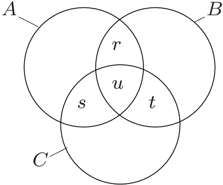
FIG. 1.: Venn diagram for a tripartite probability distribution.

Given these quantities we can express $S_{3}$ and $T_{3}$ as

$$S_{3} = r+s+t+u$$ (79)

$$T_{3} = r+s+t+2u\,\,.$$ (80)

We note that $u$ is not positive definite, but we have the positivity conditions

$$r \geq 0\ ,$$ (81)

$$s \geq 0\ ,$$ (82)

$$t \geq 0\ ,$$ (83)

$$r+u \geq 0\ ,$$ (84)

$$s+u \geq 0\ ,$$ (85)

$$t+u \geq 0\ .$$ (86)

Using these conditions, one can show that if $u=0$, then the reversible conversion

$$P_{ABC}\rightleftharpoons P^{2\otimes y_{1}}_{AB}\otimes P^{2\otimes y_{2}}_{BC}\otimes P^{2\otimes y_{3}}_{AC}$$

is allowed by our tripartite monotones. If $u>0$, then the reversible conversion

$$P_{ABC}\rightleftharpoons P^{2\otimes y_{1}}_{AB}\otimes P^{2\otimes y_{2}}_{BC}\otimes P^{2\otimes y_{3}}_{AC}\otimes P^{3\otimes y_{5}}_{ABC}$$

is allowed by our tripartite monotones. If $u<0$, then the reversible conversion

$$P_{ABC}\rightleftharpoons P^{2\otimes y_{1}}_{AB}\otimes P^{2\otimes y_{2}}_{BC}\otimes P^{2\otimes y_{3}}_{AC}\otimes P^{x\otimes y_{4}}_{ABC}$$

is allowed by our tripartite monotones.

Thus our monotones in principle allow the reversible conversion between any tripartite probability distribution and the distributions $P^{2}_{AB}$, $P^{2}_{BC}$, $P^{2}_{AC}$, $P^{x}_{ABC}$, and $P^{3}_{ABC}$. Whether or not such a reversible transformation is possible or not is an open question. To rule this out will probably require discovering additional secrecy monotones.

E Extremality of the monotones $S_{3}$ and $T_{3}$

As a final comment about the secrecy monotones in the tripartite case, we note that using the distillation procedures for ${P^{x}_{ABC}}\rightarrow P^{2}_{AB}$ and ${P^{3}_{ABC}}\rightarrow P^{2}_{AB}$, we can now also prove that $0\leq\lambda\leq 1$ is the only range for which the linear combination of $S_{3}$ and $T_{3}$ is a monotone. This can be seen by calculating $M_{3}=\lambda S_{3}+(1-\lambda)T_{3}$ for both distillations. In the first case, we get that $M_{3}(P^{x}_{ABC})=\lambda+1$ should be greater or equal to $M_{3}(P^{2}_{AB})=1$, so that $\lambda\geq 0$. In the second case, we find that $M_{3}(P^{3}_{ABC})=2-\lambda\geq M_{3}(P^{2}_{AB})=1$, so that $\lambda\leq 1$. This suggests that if there are other monotones than the $M_{n}$’s, they will probably not be composed out of entropies.

V Quantum multipartite secrecy monotones

A Definition of Quantum Secrecy Monotones

The definition of classical secrecy monotone of Section II A can be immediately extended to the quantum case. The monotone will now be a function defined on multi-partite density matrices $\rho_{A_{1}\ldots A_{n}}$ which must be:

• positive,

• vanishing on product density matrices,

• monotonous under local operations (local CP maps),

• monotonous under classical communication,

• additive,

• continous.

One can also extend the quantum definition of the secrecy monotone to the case where there is an eavesdropper. In that case, it is defined on a multipartite density matrix $\rho_{A_{1}\ldots A_{n}E}$. The monotonicity properties are then modified to require that the secrecy montone is monotonically decreasing under local operations and public communication by the parties $A_{1}\ldots A_{n}$ and monotonically increasing under local operations and public communication by Eve.

In what follows, we shall for simplicity not include Eve in the discussion. That is, we shall suppose that initially Eve has no information about the density matrix, but she listens to all public communications and thereby tries to thwart the parties $A_{1}\ldots A_{n}$.

B Quantum version of the secrecy monotones $S_{n}$ and $T_{n}$

The definitions of the monotones $S_{n}$ and $T_{n}$, Eqs. (18) and (LABEL:mon2), have straightforward generalizations to the quantum case:

$$S_{n}(\hat{\rho}_{A_{1}\cdots A_{n}})$$ (87)

$$\equiv S(A_{1}{\rm:}\cdots{\rm:}A_{n})$$ (88)

$$= \sum_{i=1}^{n}S(\hat{\rho}_{A_{1}\cdots A_{i-1}A_{i+1}\cdots A_{n}})-(n-1)S(\hat{\rho}_{A_{1}\cdots A_{n}})$$ (89)

and

$$T_{n}(\hat{\rho}_{A_{1}\cdots A_{n}})$$ (90)

$$\equiv T(A_{1}{\rm:}\cdots{\rm:}A_{n})$$ (91)

$$= \sum_{i=1}^{n}S(\hat{\rho}_{A_{i}})-S(\hat{\rho}_{A_{1}\cdots A_{n}})\,\,,$$ (92)

where now $S(\hat{\rho})$ denotes the von Neumann entropy of a density matrix which is given by $S(\hat{\rho})=-{\mathrm{Tr}}(\hat{\rho}\log\hat{\rho})$ and partial traces are written in the form $\hat{\rho}_{A_{1}\cdots A_{i-1}A_{i+1}\cdots A_{n}}={\mathrm{Tr}}_{A_{i}}(\hat{\rho}_{A_{1}\cdots A_{n}})$.

The different rewritings of $S_{n}$ [Eqs. (16), (20), and (22)] and $T_{n}$ [Eqs. (31) and(33)] that where obtained in the classical case carry through to the quantum case, in analogy to the what was shown for bipartite systems in [13]. This means that the simple properties that followed from these rewritings in the classical case also hold in the quantum case. In particular, the positivity of the $S_{n}$ and $T_{n}$ follows from the positivity of the conditional mutual entropy, which holds in both the classical and quantum case (see [17] for a review). The proofs of monotonicity change in the quantum case, and we give them below.

Let us note that, for pure states, $S_{n}$ and $T_{n}$ coincide and are equal to the sum of the local entropies:

$$S_{n}(|\psi_{A_{1}\cdots A_{n}}\rangle) = T_{n}(|\psi_{A_{1}\cdots A_{n}}\rangle)$$ (93)

$$= \sum_{i=1}^{n}S(\hat{\rho}_{A_{i}})\ .$$ (94)

Thus for instance on a singlet state, $S_{2}$ and $T_{2}$ are equal to 2, and on a GHZ state, $S_{3}$ and $T_{3}$ are equal to 3.

We do not at present have a clear interpretation of $S_{n}$ in the quantum case. On the other hand, the interpretation of $T_{n}$ in the quantum case is the same as in the classical case. Indeed, it can be written as the minimum relative entropy between $\hat{\rho}_{A_{1}\ldots A_{n}}$ and a product density matrix $\hat{\eta}_{A_{1}}\otimes\ldots\otimes\hat{\eta}_{A_{n}}$ (the minimum being attained when $\hat{\eta}_{A_{i}}=\hat{\rho}_{A_{i}}$). Therefore, $T_{n}$ can be interpreted as the minimum increase of entropy of local (uncorrelated) environnements if the parties erase all correlations between them by letting their quantum systems interact with a local environment.

C Monotonicity of $S_{n}$ and $T_{n}$

We now give the proofs of monotonicity of $S_{n}$ and $T_{n}$ under local operations and classical communication in the quantum case.

Local operations of one party are described mathematically as completely positive (CP) local maps $M_{A_{i}}$, which only act on the subspace of the $i$th party. We can assume that such a map is implemented as follows [19, 20]: $A_{i}$ adds to its Hilbert space an auxiliary variable in a pure state $\Pi_{\mathrm{aux}}=|0\rangle_{\mathrm{aux}}\langle 0|$. It then carries out a unitary transformation $\hat{U}_{i\mathrm{aux}}$ on its original system and the auxiliary variable. Finally, it traces over a part aux^′ of her Hilbert space. Note that aux^′ does not have to coincide with aux. Hence, we can represent a local CP map as

$$\tilde{\rho}_{A_{1}\cdots A_{n}} = M_{A_{i}}\otimes\openone_{A_{1}\cdots A_{i-1}A_{i+1}\cdots A_{n}}(\hat{\rho}_{A_{1}\cdots A_{i}})$$ (95)

$$= {\mathrm{Tr}}_{\mathrm{aux}^{\prime}}\left[(\hat{U}_{A_{i}{\mathrm{aux}}}\otimes\openone_{A_{1}\cdots A_{i-1}A_{i+1}\cdots A_{n}})\right.$$ (98)

$$\left.(\hat{\rho}_{A_{1}\cdots A_{n}}\otimes\Pi_{\mathrm{aux}})\right.$$

$$\left.(\hat{U}^{\dagger}_{A_{i}\mathrm{aux}}\otimes\openone_{A_{1}\cdots A_{i-1}A_{i+1}\cdots A_{n}})\right]\,\,.$$

We start with $S_{n}$ and write it in the following form

$$S_{n}(A_{1}{\rm:}\cdots{\rm:}A_{n})$$ (99)

$$= \sum_{i=1}^{n-1}S_{2}(A_{i}{\rm:}A_{1}\cdots A_{i-1}A_{i+1}\cdots A_{n-1}A_{n})$$ (101)

$$-{}\Delta_{n}\,\,,$$

with

$$\Delta_{n}=\sum_{i=1}^{n-1}S(\hat{\rho}_{A_{i}})-S(\hat{\rho}_{A_{1}\cdots A_{n-1}})\,\,.$$ (102)

Now we assume that the system $A_{n}$ undergoes a local CP map $M_{n}$, Eq. (98). As $\Delta_{n}$ does not depend on $A_{n}$ it remains unchanged, thus we only have to check $S_{2}$ for monotonicity. For this we rewrite Eq. (98) for two systems $A$ and $B$

$$\tilde{\rho}_{AB} = M_{A}\otimes\openone_{B}(\rho_{AB})$$ (103)

$$= {\mathrm{Tr}}_{a^{\prime}}(U_{Aa}\otimes\openone_{B})\rho_{AB}\otimes\Pi_{a}(U_{Aa}^{\dagger}\otimes\openone_{B})$$ (104)

and note that neither adding a local auxiliary nor performing a unitary transformation changes $S_{2}$. Tracing over a local subsystem, however, decreases $S_{2}$ since

$$S_{2}(A^{\prime}{\mathrm{aux}}^{\prime}{\rm:}B)-S_{2}(A^{\prime}{\rm:}B)$$ (105)

$$= S({\mathrm{aux}}^{\prime}{\rm:}B|A^{\prime})\,\,,\hskip 85.35826pt$$ (106)

which is just the conditional mutual quantum entropy and which, due to strong subadditivity [17] is semipositive, thus implying that

$$S_{2}(A^{\prime}{\mathrm{aux}}^{\prime}{\rm:}B)\geq S_{2}(A^{\prime}{\rm:}B)\,\,.$$ (107)

Due to symmetry, $S_{n}$ given by Eq. (101) is then monotone under local CP maps of any party.

For monotonicity under local measurements and public communication of their outcome, we assume that a positive operator valued measurement (POVM) [20] is performed on system $A_{1}$. This is realized by adding as above an ancilla $\Pi_{\mathrm{aux}}$ to $A_{1}$ and then carrying out a von Neumann measurement that transforms $\hat{\rho}_{A_{1}\cdots A_{n}}\otimes\Pi_{\mathrm{aux}}$ to

$$\tilde{\rho}_{{\mathrm{aux}}A_{1}\cdots A_{n}}=\sum_{k}\hat{\rho}^{k}_{{\mathrm{aux}}A_{1}\cdots A_{n}}=\sum_{k}p_{k}\tilde{\rho}^{k}_{{\mathrm{aux}}A_{1}\cdots A_{n}}\,\,,$$ (108)

with $\hat{\rho}^{k}_{{\mathrm{aux}}A_{1}\cdots A_{n}}=(\hat{P}^{k}_{{\mathrm{aux}}A_{1}}\otimes\openone_{A_{2}\cdots A_{n}})(\hat{\rho}_{A_{1}\cdots A_{n}}\otimes\Pi_{\mathrm{aux}})(\hat{P}^{k}_{{\mathrm{aux}}A_{1}}\otimes\openone_{A_{2}\cdots A_{n}})$ and $\hat{P}^{k}_{{\mathrm{aux}}A_{1}}$ a complete set of orthogonal projectors acting on the extended space ${\mathrm{aux}}A_{1}$, $\tilde{\rho}^{k}_{{\mathrm{aux}}A_{1}\cdots A_{n}}$ being the joint state after outcome $k$ has been measured and $p_{k}={\mathrm{Tr}}(\hat{\rho}^{k}_{{\mathrm{aux}}A_{1}\cdots A_{n}})$. We now go back to Eq. (89). The orthogonality of the projectors $\hat{P}^{k}_{{\mathrm{aux}}A_{1}}$ implies that the $\tilde{\rho}_{A_{1}\cdots A_{i-1}A_{i+1}\cdots A_{n}}$ are block diagonal for $i\neq 1$, so that their entropies can be expressed as

$$S(\tilde{\rho}_{A_{1}\cdots A_{i-1}A_{i+1}\cdots A_{n}}) = H[p_{k}]$$ (110)

$$+{}\sum_{k}p_{k}S(\tilde{\rho}^{k}_{A_{1}\cdots A_{i-1}A_{i+1}\cdots A_{n}})\,\,,$$

and

$$S(\tilde{\rho}_{A_{1}\cdots A_{n}}) = H[p_{k}]+\sum_{k}p_{k}S(\tilde{\rho}^{k}_{A_{1}\cdots A_{n}})\,\,,$$ (112)

with $H[p_{k}]$ denoting the classical Shannon entropy of the probability distribution $p_{k}$. For $i=1$, we find the following inequality for the first term, which makes use of the concavity of entropy

$$S(\tilde{\rho}_{A_{2}\cdots A_{n}})\geq\sum_{k}p_{k}S(\tilde{\rho}^{k}_{A_{2}\cdots A_{n}})\,\,.$$ (113)

Replacing all these expressions in Eq. (18), we finally find that

$$S_{n}\left(\sum_{k}p_{k}\tilde{\rho}_{A_{1}\cdots A_{n}}^{k}\right)\geq\sum_{k}p_{k}S_{n}(\tilde{\rho}_{A_{1}\cdots A_{n}}^{k})\,\,.$$ (114)

This shows that the monotone $S_{n}$ can only decrease on average if $A_{1}$ performs a POVM measurement and the outcome is made known to the other parties. By symmetry, this property holds for all $A_{i},i=\{1,\ldots,n\}$.

To prove the monotonicity of $T_{n}$ we proceed as follows. Suppose that $A_{1}$ carries out a local CP map. As before adding a local ancilla and carrying out a local unitary transformation do not change $T_{n}$. Tracing over part of $A_{1}$’s Hilbert space decreases $T_{n}$. Indeed, $T_{n}(A_{1}a_{1}{\rm:}A_{2}{\rm:}\cdots{\rm:}A_{n})-T_{n}(A_{1}{\rm:}\cdots{\rm:}A_{n})=S(a_{1}{\rm:}A_{2}\ldots A_{n}|A_{1})\geq 0$. Suppose now that $A_{1}$ carries out a measurement (with outcomes $k$) and publicly reveals the result. In Eq. (92), the terms $S(\rho_{A_{i}})$ with $i\neq 1$ decrease because of concavity of entropy [see Eq. (113)] and because the term $S(\rho_{A_{1}})-S(\rho_{A_{1}\ldots A_{n}})$ stays constant [where we used Eqs. (LABEL:cond1) and (112)]. Hence,

$$T_{n}\left(\sum_{k}p_{k}\tilde{\rho}_{A_{1}\cdots A_{n}}^{k};A_{1}:\cdots:A_{n}\right)$$ (115)

$$\geq \sum_{k}p_{k}T_{n}(\tilde{\rho}_{A_{1}\cdots A_{n}}^{k};A_{1}:\cdots:A_{n})$$ (116)

where we have used the same notation as in Eq. (114).

D Applications of quantum secrecy monotones

The two quantum monotones described above can be used to provide bounds on the rate of conversion of one multipartite density matrix into another using local operations and classical communication. As an example, we study in this section and the next one how many realizations of a correlated tripartite probability distributions can be obtained from a GHZ state.

Let us recall that the GHZ state, in the $z$ basis, is

$$|GHZ\rangle=(|000\rangle+|111\rangle)/\sqrt{2}\ .$$

If the state is measured in the $z$ basis one obtains the probability distribution $P^{3}$. In contrast, if the state is measured in the $x$ basis one obtains the probability distribution $P^{x}$.

We have shown above that $P^{3}$ and $P^{x}$ cannot be reversibly converted one into the other. This therefore suggests that when using a GHZ state to do multipartite quantum cryptography, there is an irreversible choice that must be made. However, the above discussion leaves open the possibility that the three parties could use a more sophisticated strategy than the ones just described and thereby obtain more than one of these probability distributions from a single GHZ state.

To address this question, let us compute the monotones $S_{3}$ and $T_{3}$ on the initial state and on the final probability distributions. We find

$$S_{3}(|GHZ\rangle)=3\quad \quad T_{3}(|GHZ\rangle)=3\ ,$$ , (117)

$$S_{3}(P^{3})=1\quad \quad T_{3}(P^{3})=2\ ,$$ , (118)

$$S_{3}(P^{x})=2\quad \quad T_{3}(P^{x})=1\ .$$ , (119)

Thus the monotones leave open the possibility of a higher yield than one $P^{3}$ or one $P^{x}$ per GHZ state.

Let us note however an interesting feature of eq. (119), namely that the sum of the final values of $S_{3}$ and $T_{3}$ is equal to half the sum of the initial values:

$$S_{3}(P^{3})+T_{3}(P^{3}) = S_{3}(P^{x})+T_{3}(P^{x})$$ (120)

$$= {S_{3}(|GHZ\rangle)+T_{3}(|GHZ\rangle)\over 2}\ .$$ (121)

We shall now show that this is no accident but is necessarily the case when one passes from a multipartite pure state to a multipartite probability distribution. Thus it is indeed impossible to obtain more than one $P^{3}$ or one $P^{x}$ probability distribution from a single GHZ state, and the simple measurement strategies described above are therefore optimal.

E Decrease of $S_{n}+T_{n}$ when passing from a multipartite pure state to a multipartite probability distribution

Let us suppose that initially the parties share a multipartite pure state $|\Psi_{A_{1}\ldots A_{n}}\rangle$. Initially

$$S_{n}(\|Psi_{A_{1}\ldots A_{n}}\rangle)=T_{n}(|\Psi_{A_{1}\ldots A_{n}}\rangle)=\sum_{i}S(\rho_{A_{i}})\ .$$ (122)

Suppose that the aim of the parties is to obtain, by carrying out local measurements and classical communication, a multipartite probability distribution $P_{A_{1}\ldots A_{n}}$. In doing so, the monotones $S_{n}$ and $T_{n}$ will decrease. More precisely, the amount by which they decrease is such that their sum is decreased by at least a factor two:

$$S_{n}(P_{A_{1}\ldots A_{n}})+T_{n}(P_{A_{1}\ldots A_{n}})\leq\sum_{i}S(\rho_{A_{i}})\ .$$ (123)

To prove this, let us first consider the bipartite case. Thus initially the parties share a pure state $|\Psi_{AB}\rangle$ and they carry out measurements so as to obtain a probability distribution $P_{AB}$. Let us first suppose that no communication takes place between the parties. Then, it follows from Holevo’s bound[18] that the mutual information between Alice and Bob after the measurement is necessarily less than the local entropies of the original state:

$$S(\rho_{A})=S(\rho_{B})\geq I_{P_{AB}}(A{\rm:}B)\ .$$ (124)

Equality is attained in Eq. (124) only if they measure in the Schmidt basis.

Let us now show that Eq. (124) also holds if the parties communicate classically. We will suppose that the communication takes place in a series of rounds. During each round, one of the parties carries out a partial measurement on the state and communicates information to the other party. After all the communication has taken place the parties measure the state they are left with. Such a general protocol is difficult to analyze, but we can transform it into a simpler protocol. In the simpler protocol, during each round the party transmits all the information obtained by the partial measurement to the other party. This should be contrasted with the most general protocol in which only part of the information obtained by the measurement is transmitted. The simplification follows from the fact that we can divide the measurement into a first partial measurement in which the information transmitted to the other party is obtained, and a second partial measurement in which the information that is kept is obtained. But the second partial measurement could then as well be carried out during the next round. Repeating this reasoning round after round, we can construct a simpler protocol in which the information that is not communicated to the other party is acquired during the last round only.

In the case of the simplified protocol, one can easily show that Eq. (124) holds. Consider the first round. Suppose that Alice carries out a partial measurement. The measurement has outcomes $k$, with probabilities $p(k)$. The state if the outcome is $k$ is $\Psi_{AB}^{k}$. Because of monotonicity of the quantum mutual information, we have

$$S(\rho_{A})\geq\sum_{k}p(k)S(\rho_{A}^{k})\ .$$ (125)

The local entropies decrease (on average) due to the communication. The same will hold for all the subsequent rounds. Hence, Eq. (124) holds also if the parties carry out public communication. In fact that above reasoning shows that the optimal strategy is for the parties not to communicate, but simply to measure the state in the Schmidt basis.

Finally let us consider the multipartite case. The result for two parties Eq.(124) implies that for any partition of the parties into one party, say $i$, and $n-1$ parties, the mutual information between $i$ and the $n-1$ other parties after the measurements is bounded by

$$I(A_{i}{\rm:}A_{1}\ldots A_{i-1}A_{i+1}\ldots A_{n})\leq S(\rho(A_{i}))\ .$$ (126)

Summing over $i$ and using Eq. (37), we find that

$$S_{n}(P)+T_{n}(P)\leq\sum_{i}S(\rho(A_{i}))$$ (127)

which is what we wanted to prove.

VI Conclusion

In this article, we have introduced the concept of secrecy monotones which are powerful tools to obtain bounds on the distillation rate in Maurer’s classical cryptographic scheme as well as bounds on the distillation rate in quantum cryptography.

We introduced two independent multipartite secrecy monotones based on (Shannon or von Neuman) entropies, $S_{n}$ and $T_{n}$, which allowed us to investigate the distillation rates for multipartite cryptographic schemes. In the classical case, we studied in detail the tripartite case and showed that their are several inequivalent tripartite probability distributions in the sense that they cannot be converted reversibly one into the other. We also studied the particular case of tripartite quantum cryptography based on the GHZ state. We showed that the parties must choose a priori which probability distribution they want to generate.

The important feature that emerges from our study is thus that in multipartite classical or quantum cryptography, the parties must make an irreversible choice on what final probability distribution they want to obtain. Making the wrong choice entails an irreversible loss. We note that this feature is not unique to cryptography; indeed, a similar situation arises in multipartite entanglement distillation since there are entangled pure states that cannot be reversibly converted one into the other[7, 8].

Note: After this paper was completed, we learned of the work [21] in which monotones (under certain classes of operations) which are positive both on quantum states and on probability distributions are considered in the bipartite case.

Acknowledgements: We would like to thank Nicolas Gisin and Daniel Collins for helpful conversations. We acknowledge funding by the European Union under the project EQUIP (IST-FET programme). S.M. is a research associate of the Belgian National Fund for Scientific Research.

REFERENCES

- [1] Ch. H. Bennett and G. Brassard, Int. Conf. Computers, Systems and Signal Processing, Bangalore, India, December 10-12, pages 175-179 (1984)
- [2] N. Gisin, G. Ribordy, W. Tittel, H. Zbinden, Quantum Cryptography, quant-ph/0101098
- [3] U. Maurer, IEEE Transactions on Information Theory, Vol. 39, No. 3, pp. 733-742, 1993
- [4] U. Maurer and S. Wolf, IEEE Transactions on Information Theory, Vol. 45, No. 2, pp. 499-514, 1999
- [5] N. Gisin and S. Wolf, Phys. Rev. Lett. 83 (1999) 4200
- [6] N. Gisin and S. Wolf, Linking Classical and Quantum Key Agreement: is there “Bound Information”?, quant-ph/0005042
- [7] C. H. Bennett, S. Popescu, D. Rohrlich, J. A. Smolin, and A. V. Thapliyal, Phys. Rev. A 63 (2001) 012307
- [8] N. Linden, S. Popescu, B. Schumacher, M. Westmoreland, Reversibility of local transformations of multiparticle entanglement, quant-ph/9912039
- [9] E. F. Galvao, M. B. Plenio, S. Virmani, J. Phys. A 33, 8809 (2000)
- [10] M. B. Plenio, V. Vedral, Bounds on relative entropy of entanglement for multi-party systems, J. Phys. A 34, 6997 - 7002 (2001)
- [11] M. Horodecki, P. Horodecki, R. Horodecki, Phys. Rev. Lett. 84 (2000) 2014
- [12] N. J. Cerf and C. Adami, Phys. Rev. Lett. 79, 5194 (1997); Physica D 120, 62 (1998).
- [13] C. Adami and N. J. Cerf, Phys. Rev. A 56, 3470 (1997); N. J. Cerf, Phys. Rev. A 57, 3330 (1998).
- [14] V. Vedral, Landauer’s erasure, error correction and entanglement, quant-ph/9903049, to appear in The Proceedings of The Royal Society
- [15] V. Vedral, The Role of Relative Entropy in Quantum Information Theory, quant-ph/0102094
- [16] T. M. Cover and J. A. Thomas, Elements of Information Theory, (John Wiley & Sons, New York, 1991).
- [17] A. Wehrl, Rev. Mod. Phys. 50, 221 (1978).
- [18] A. S. Holevo, Problemy Peredachi Informatsii 9, 3 (1973)
- [19] B. Schumacher Phys. Rev. A 54, 2614-2628 (1996)
- [20] K. Kraus, States, Effects, and Operations, Springer, Berlin, 1983.
- [21] B. M. Terhal, M. Horodecki, D. W. Leung, D. P. DiVincenzo, The entanglement of purification, quant-ph/0202044