MATHEMATICAL PHYSICS AND LIFE

Abstract

It is a fascinating subject to explore how well we can understand the processes of life on the basis of fundamental laws of physics. It is emphasised that viewing biological processes as manipulation of information extracts their essential features. This information processing can be analysed using well-known methods of computer science. The lowest level of biological information processing, involving DNA and proteins, is the easiest one to link to physical properties. Physical underpinnings of the genetic information that could have led to the universal language of 4 nucleotide bases and 20 amino acids are pointed out. Generalisations of Boolean logic, especially features of quantum dynamics, play a crucial role.

1 What is Life?

Often life is characterised on the basis of its fundamental processes: metabolism and reproduction. But perhaps it is easier to characterise what life is not than to define what it is. Life is not a process of thermodynamic equilibrium—all the metabolic activities are driven by a continuous supply of energy which is obtained from the environment as food. Evolution of life is not dictated by precise rules of logic—it is governed by random events where memory plays a role but there is no foresight. Living organisms are made of neither completely regular arrangements as in a solid nor totally random arrangements as in a gas—all the activities take place in a liquid medium with continuous jostling amongst various biomolecules. These properties make the familiar tools of physicists—equilibrium dynamics, axiomatic deductions, periodic structures, perturbation theory—totally useless when it comes to understanding life. Life is termed too nonlinear, too complex, too unwieldy for the simple tools of physicists to handle.

Information theory provides a way out of this apparently hopeless conundrum. Information is the abstract mathematical concept that quantifies the notion of order amongst the building blocks of a message. It extracts just the right features from the apparently chaotic ensemble that is life, and allows the study of its manipulations without going into the nitty-gritty of all the details. Of course, figuring out the appropriate information in a given process requires detailed experiments and modeling. But once the essential features have been extracted, the rules of information processing are precise enough to allow their systematic analysis in a mathematical framework.

It can be argued that information processing is not just a particular characteristic of living organisms, but it is their most important characteristic [1]. The processes of life are aimed towards survival of the organism. Even though we do not quite understand why the organisms want to perpetuate themselves, we have enough evidence to show that they use all available means for this purpose [2]. The damage caused by the disturbances from the environment makes it impossible for a particular individual to survive forever, so the perpetuation is carried out through the process of replication. In this process, the knowledge gathered on how to survive is carried forward from one generation to the next. The pattern of acquiring, interpreting and passing on information, often after using and refining it, has occurred repeatedly during evolution. The hereditary genetic information is the most basic and primitive communication system. As living organisms evolved, the lower levels of information communication have been bypassed in favour of more efficient higher level mechanisms, reducing dependence on direct physical contact at every stage. Electrochemical signaling between cells and nervous systems evolved in multicellular organisms, teaching and imitation arose amongst parents and offsprings, verbal and sign languages originated amongst members of the same species, humans created books and libraries for long term storage of information, we use telecommunication and computers nowadays, and the future (already imagined in science fiction stories) is likely to witness fusion of brains with computers.

2 Biological Information

Living organisms absorb free energy from the environment to create order from disorder. All their struggles for raw materials and energy are ultimately for picking up necessary building blocks and organising them in a desired manner. After the organisms die, the building blocks gradually come apart and become random ensembles. Quantitatively the information carried by a set of building blocks is nothing but the entropy (up to an unimportant proportionality constant), and principles of computer science can be used to study its transformations.

Table 1 lists various stages of information processing tasks carried out by living organisms and compares them with similar tasks carried out by our electronic computers. They have been arranged in a hierarchy of levels according to the physical scales involved. Different levels typically have different languages, and the processing translates the information from one level to the next. We are accustomed to looking at our computers from the top level down—from the abstract mathematical equations to the transistors embedded in the silicon chips. On the other hand, living organisms have evolved from the bottom level up—from the biomolecular interactions to multicellular systems.

Living organisms	Task	Computers
Signals from environment	Input	Data
Sense organs	High level	Pre-processor
Nervous system + Brain	Translation	Operating system + Compiler
Electrochemical signals	Low level	Machine code
Proteins	Execution	Electrical signals
DNA	Programme	Programmer

Table 1: Hierarchical processing of information in living organisms and in computers.

To understand the working of an information processing system, one must figure out what happens at each level step by step. But where should one begin, when little is known about the system? At this juncture, it is worthwhile to observe that two major simplifications occur as one proceeds from high level information processing to low level:
(1) The languages at the higher levels are abstract software. They get translated from one to another according to established conventions. On the contrary, the languages at the lowest levels are directly connected to the physical responses of the hardware. There is no more translation of the message—the interpretation of the signal is built into the design of the system and not left to an external agency. (e.g. we can programme the mathematical formulae into the computer in a variety of notations, but ultimately they are all converted to pulses of voltages and currents because the transistors in the silicon chips cannot respond to any other language.)
(2) The abstract high levels allow a variety of subjective choices in the languages. That leads to lots of variations, historical adaptations and a large number of possible instructions. At the lowest level, only a handful of instructions related to physical responses of the hardware are possible, and the language tends to become universal. (e.g. for writing the computer programmes, we may choose between Fortran and C, or Unix and Windows, but finally all that is reduced to the operations of Boolean logic.)

These properties make it obvious that it is easiest to decipher an information processing system at the lowest level, where the physical properties of the hardware dictate the language and the instructions [3]. Complex systems are then generated by putting together a large number of simple ingredients. With the progressive miniaturisation of the silicon chips, the lowest level of information processing in our computers nowadays is at the scale of a micron. The lowest level of information processing for the living organisms is at the molecular scale—a scale smaller by a factor of thousand. The molecules involved there are DNA and proteins, and their language is universal—the same all the way from viruses and bacteria to human beings. So our first objective is to identify the information processing tasks carried out by DNA and proteins, and then study the relation between these tasks and physical properties of the molecules. It is important to note that biological systems are not general purpose computers, where the same CPU handles all the tasks. Living organisms have evolved specialised components to perform specific tasks, which makes it easy to identify the task of a component and study its implementation in detail.

DNA is the read-only-memory of the living organisms. It is a linear chain constructed from an alphabet of 4 nucleotide bases. Most of the time, the information carried by it remains nicely protected in the double helical structure. Whenever necessary, the information is “copied” into another DNA molecule during replication and mRNA molecule during transcription. The “copying” is not literal, rather it follows rules of complementary base-pairing. The “copy” is assembled on the master template, by picking up desired nucleotide bases one by one from the surroundings and joining them together in a chain. The available nucleotide bases are floating around randomly in the cell, and the base-pairing rules decide which one is the correct one to insert at a specific location. Thus the only task carried out by DNA is the sequential assembly of a chain of nucleotide bases, selected from a random ensemble.

Proteins carry out almost all the processes required by the living cell, by binding to various molecules. The binding is highly specific, very much like a lock and key mechanism. For this purpose, proteins contain structurally stable features, precisely located on the surface. Each protein has its own unique shape and participates in its own unique process. Proteins are made of one or more tightly folded polypeptide chains (they may contain other ingredients but the role of these other ingredients is essentially chemical and not structural). Polypeptide chains are synthesised from an alphabet of 20 amino acids, and other ingredients get added afterwards. Each polypeptide chain is assembled on the mRNA template during translation when successive segments of 3 nucleotide bases are mapped onto individual amino acids. Every chain subsequently folds up into a three-dimensional structure, uniquely determined by its amino acid sequence. The proteins are thus involved in two information processing tasks. One is similar to that of DNA, i.e. sequential assembly of a chain of amino acids selected from a random ensemble. The other is to create a multitude of three-dimensional structures by folding up linear polypeptide chains.

These tasks are carried out at the molecular scale. We know the physical laws applicable there—classical dynamics is relevant, but atomic structure and quantum dynamics cannot be ignored. We can now pose the question: were we to design a processor to carry out the tasks of DNA and proteins, what design would we come up with knowing all that we do about the physical laws? The rest of the article investigates this question, and compares the results to what is found in nature.

3 Survival of the Fittest

It is advantageous to process the information efficiently, and not in any haphazard manner. The first attempt may not provide the best solution to a problem, but the attempts do not stop there. Technological developments are driven as much by new inventions as by untiring attempts to improve and optimise earlier solutions. In general, information processing is optimised following two guidelines: minimisation of physical resources (time, space, energy etc.) and minimisation of errors. These guidelines often impose conflicting demands on the solution, and specific trade-offs are made depending on the details of the problem.

In case of living organisms, the optimisation criteria are paraphrased as “Darwinian evolution”. The environment and competition drive the living organisms to adapt to them by exerting selection pressures, and we can illustrate that by many examples. We now understand the genetic basis behind Darwinian evolution. No information processing system can be perfect, and occasional errors in genetic information processing produce random mutations of living organisms. The error rate is bound to be small in any reasonably stable system, and mutations are small local fluctuations in DNA molecules. The mutated organism is in essentially the same environment as the original one, and both have to compete for the available resources. If the mutation improves the ability of the organism to survive, the mutated organism grows in number, otherwise it fades away. To what extent may all this be quantified?

Let the index $i$ label a set of coexisting species in a given environment, and let $\phi_{i}(t)$ denote their populations at time $t$. The simplest evolution scenario is where the future population of each species depends linearly on the present populations of all the species,

$$\phi_{i}(t+1)=\sum_{j}M_{ij}\phi_{j}(t)~{},~{}~{}\phi_{i}(t)\geq 0~{}.$$ (1)

The diagonal terms $M_{ii}$ represent the individual rates of growth, while the off-diagonal terms $M_{i\neq j}$ represent interactions between species. Every species consumes resources from the environment; when the available resources are limited, the total population cannot exceed a certain value (a normalisation convention can be chosen such that a unit of each species utilises the same amount of resources). Evolution gets really competitive when the total population reaches its maximum value. In this stage,

$$\sum_{i}\phi_{i}(t)=N~{},~{}~{}\sum_{i}M_{ij}=1~{}.$$ (2)

Evolutionary models obeying Eqs.(1,2) have often been used together with the constraint $0\leq M_{ij}\leq 1$. They describe Markovian evolution in the language of classical probability theory. With the constraints on $M_{ij}$, one can prove many inequalities and convergence properties. This is not the interesting part of evolution, however.

Fixed amount of available resources correspond to conservation laws. The most general evolution in such circumstances is described by “orthogonal transformations” [4]. The generators for these transformations are antisymmetric matrices. Thus in a general evolutionary setting, it is more appropriate to let $M_{ij}$ take positive as well as negative values. As a matter of fact, situations of both positive and negative feedback occur routinely in biological systems (e.g. catalysis and inhibition, symbiosis and parasitic behaviour, defence mechanisms and cancer, etc.). When the resources are limited, one gains only at the expense of someone else—the formal setting is called “zero-sum games”.

We can now look at how evolution changes, when the range of $M_{ij}$ is extended to include negative values. Clearly extending the range of $M_{ij}$ cannot make the evolutionary algorithm any less efficient. On the contrary, recent developments in quantum computation [5] offer a hint. Quantum algorithms exploit two features to beat their classical counterparts, superposition of states and cleverly designed destructive interference. Superposition means letting all the states be in the same place at the same time, and it can reduce the spatial resources required for the algorithm exponentially. But superposition is not an option available to coexisting biological species. Even in absence of superposition, destructive interference can be used to eliminate undesired states and to reach the output state more quickly. The execution time is reduced at least by a constant factor if not polynomially. Biological evolution occurs over long time scales, and even a tiny change in the rate of growth is important because it can translate into exponential changes in populations over a long time. Negative values of $M_{ij}$ can indeed be interpreted as effects of destructive interference, which help the species reach their asymptotic populations faster. The lessons learnt from quantum computation then tell us that “orthogonal transformations” offer a quicker way of picking a winner amongst the contenders. These arguments are not a rigorous derivation, but they allow us to infer that competition beats altruism and Darwinian selection is a consequence of limited availability of resources [6].

Exercise: Study evolution algorithms governed by Eqs.(1,2). Estimate the speed-up obtained when $M_{ij}$ are allowed to become negative compared to when they are restricted to be positive.

Having justified that optimisation principles do play a role in biological systems, let us analyse what is optimised and how. In designing more and more efficient computers, we have explored the criteria mentioned at the beginning of this section. To optimise spatial resources, we need elementary hardware components that are simple and easily available, and yet versatile enough to be connected together in many different ways. This is the typical choice made at the lowest level of information processing, and complicated systems are then constructed by packing a large number of components in a small volume. It helps to have a small number of elementary components, because that reduces the number of possible instructions and the connections amongst the components. With a small instruction set, individual steps can be implemented quickly and the time required for processing information is cut down. In addition to these, in the implementation of any given task, we have to find a software algorithm which requires smallest number of components and smallest number of execution steps.

For our computers, it is also necessary to minimise the energy consumption during processing. But this feature is surprisingly absent in biological systems. The reason is that the elementary components of biological systems are so simple and cheap, that they carry out their tasks with very little energy—a single biomolecular interaction requires a million times less energy than a Boolean logic operation with modern silicon transistors. As a result, biological systems often exhibit a wasteful feature. Millions of eggs and pollen grains are produced when a few would have sufficed to propagate the species in a secure environment. Such overkills strengthen the competition and enforce survival of the fittest.

Exercise: Observe that biological systems have evolved excellent amplifiers for processing occurring at the molecular scale. Eyes and chlorophyll can detect a few photons, smells can be identified with a few molecules and sound amplitudes with a fraction of atomic size can be heard. Body movements almost always use levers in the configuration of mechanical disadvantage; it is somewhat ironic that mechanical advantage corresponds to gain in power which is the reciprocal of the gain in amplification. Obtain quantitative data for such amplification processes.

Faithful information processing requires that the error rate must be kept in control. One strategy is to shield the system from unwanted external disturbances, but that does not protect against internal fluctuations. Internal errors are minimised by selecting an information processing language based on discrete variables (as opposed to continuous variables). Allowed values of fundamental physical variables are often continuous, in which case a set of non-overlapping intervals of values can be chosen as the discrete variables. This is the common procedure of digitisation. The advantage is that the discrete variables remain unaffected, even when the underlying continuous variables drift, as long as the drifts keep the values within the assigned intervals. As a matter of fact, digitisation allows elimination of bounded errors. When the discrete variables are chosen as far apart from each other as possible in a given range of values, misidentification is minimised and one has the largest protection against errors. Even with digitisation, errors from large fluctuations cannot be eliminated. It is a curious fact that biological systems take advantage of a tiny error rate—with too many errors the organism will not be able to survive, but without mutations there will be no evolution.

4 Choice of Language

We are now in a position to look at some examples of information processing systems, and understand how well they implement the optimisation principles. Table 2 lists some of the languages used by living organisms, their basic components and the operations performed on those components. Messages are constructed by linking the basic components—the building blocks of the language—in a variety of arrangements. The information contained in a message depends on the values and locations of the building blocks. Any language that communicates non-trivial information must have the flexibility to arrange its building blocks in different ways to represent different messages.

This notion is quantified by saying that messages are aperiodic chains of the building blocks, and the information contained in a message is its entropy, i.e. a measure of the number of possible forms the message could have taken [7]. This definition tells us that the information content of a message can be increased by eliminating correlations from it and making it more random. It also tells us that local errors in a message can be corrected by building long range correlations into it. But it does not tell us what building blocks are appropriate for a particular message. The choice of building blocks depends on the type of information and not on the amount of information.

Physical system	Information	Building blocks	Operations
Computer	Numerical	Digits	$Z_{n}$ (modulo-$n$ arithmetic)
Verbal languages	Positional	Syllables	$S_{n}$ (permutations)
Nervous system	Temporal	Electrical pulses	$Z_{2}$ (on/off)
Genes	Positional	Nucleotide bases	Comparison (replication)
Proteins	Structural	Amino acids	$Z\otimes T$ (translation, rotation)

Table 2: Different types of information systems and their properties.

A striking feature of all the types of information listed above is that they all have digital form. The simplicity of instructions and the control over errors offered by digitisation are too important to ignore. The fact that digitisation necessarily approximates values of continuous variables does not matter in practical applications. The reason is that no practical result needs infinite precision; as long as the results are obtained within predefined but non-zero tolerance limits they are useful [8]. The outstanding optimisation question then is to figure out the best way of digitising a message, i.e. what should be selected as the building blocks of the aperiodic chain.

When the languages are versatile enough, information can be translated from one language into another by replacing one set of building blocks by another. Nonetheless, physical principles are involved in selecting different building blocks for different information processing tasks. For example, our electronic computers compute using electrical signals but store the results on the disk using magnetic signals; the former encoding is suitable for fast processing while the latter is suitable for long term storage. It is therefore the available hardware and the job to be carried out which dictate the optimal building blocks in any information processing task.

Languages of biological systems have arisen by trial and error exploration, and by accumulation of small modifications, and not by mathematical deduction of the optimal choice. Historical baggage is often carried forward in such situations; one gets stuck in local optima without discovering the globally optimal features. The optimal solution can be reached only when there is a long enough time for exploration [9]. Biologists have often viewed the languages of genes and proteins as “frozen accident”—it is such a vital part of life that any change in it would be highly deleterious [10]. On the other hand, these languages are universal across all living organisms and exhibit efficient packing of information (little correlation or close to maximal entropy), which suggest that the optimal form may have been reached. Keeping all these ideas at the back of our mind, let us step by step search for the optimal way of implementing the tasks of DNA and proteins, and compare that to what is observed in nature.

Exercise: Understand the physical reasons behind various numerical systems we use. Why do we have binary arithmetic for computers, decimal system for counting, and even more complicated system for marking time?

5 Structure of Proteins

It is convenient to analyse the language of proteins first, since it is a straightforward exercise in classical geometry [11]. The problem is to find a discrete language than can encode arbitrary shapes in 3-dimensional space, much like designing children’s playing blocks so that they can be linked together to create many different structures. This means discretising the continuous operations of translation and rotation. At the molecular scale, the atomic structure of matter automatically provides such a discretisation of space, i.e. a lattice. Among all possible lattice discretisations, the simplest lattice unit that can faithfully describe the space in any dimension is the simplex—the volume element formed by a set of $(d+1)$ points in $d$-dimensions [12].

	1-dim	3-dim
Information	Numerical	Structural
Discrete space	Integers	Lattice
Basic variables	{0,1}	$l$={0,1}
Implementation	On/Off	Tetrahedron
Operations	Addition	Translation
	Multiplication	Rotation

Table 3: Comparison of the simplest 1-dim and 3-dim information encodings.

The changes required to go from the familiar language of 1-dimensional numerical information to the language of 3-dimensional structural information are summarised in Table 3. We can quickly observe the following facts:
$\bullet$ In 3-dimensional space, the simplex is a tetrahedron. One can go from any vertex to any other vertex by a single step. Arbitrary structures can be constructed by joining tetrahedra together.
$\bullet$ A regular tetrahedron describes four equivalent and equidistant states. They correspond to the smallest two representations of the spherical harmonics, $l=0,1$. This is the obvious generalisation of the 1-dimensional binary arithmetic to the 3-dimensional space. In quantum theory, these four states are formed by $sp^{3}$-hybridisation of atomic orbitals and provide an orthogonal basis.
$\bullet$ The ideal chemical element for realising tetrahedral geometry in molecular structures is carbon, in the form of a diamond lattice. Carbon has the capability to form aperiodic chains, where different side chemical groups hang onto a backbone, which is a must for encoding information.
$\bullet$ The carbon atom is located at the centre of the tetrahedron, with its four bonds directed towards the four vertices. The tetrahedral symmetry group $T_{d}$ has 24 elements, which can be factored into a group $T$ of 12 proper rotations and reflection (or parity). The proper rotations consist of rotations around four 3-fold axes and three 2-fold axes, and describe rotations around bonds of the central carbon atom. The parity transformation flips the chirality of the molecule, and is rare enough to be ignored in the structural analysis of proteins.
$\bullet$ The tetrahedral geometry also plays a crucial role in the properties of water—the essential solvent for all the processes of life. The proteins are often hydrated, with water molecules filling the cavities. The role of water, however, will not be pursued here.

Arbitrary irregular shapes can be constructed by gluing tetrahedra together, similar to how children assemble their playing blocks. But such a process has to rely on an external agency to stop the growing process when the desired structure has been reached. At the lowest level of information processing, there is no luxury of an external agency—the building blocks themselves have to carry the information about the required shape. The solution is to encode the 3-dimensional structural information as a 1-dimensional chain that knows how to bend and fold at every step. (The assembly problem, which cannot do without an external agency, then simplifies—only 1-dimensional chains have to be assembled, and we will look at that later.) This is the solution chosen by nature. The other advantage of constructing proteins as chains which can fold and unfold is that they can cross membranes and cell walls, which they need to do to participate in various cellular processes, without making big holes in them. It is a marvelous piece of engineering that proteins unfold to their chain form, cross the membrane through a small hole that prevents other objects from leaking, and then fold again into their characteristic shapes.

5.1 The polypeptide backbone

To have the capability to fold and unfold the backbone of the chain must be strong and its side interactions weak. The simplest backbone formed by a string of carbon atoms is that of polyethylene (i.e. $(-CH_{2}-)_{n}$). It is made of rotatable carbon-carbon single bonds, and is too flexible to hold its shape. The rigidity of the backbone can be increased by including in it some double bonds that cannot rotate; the backbone will then have stiff segments alternating with flexible joints similar to a chain of metal rings. The simplest such non-planar backbone is formed by alternating one double bond with two single bonds. That is the backbone of polypeptide chains—the stiff $C-N$ peptide bond increases its rigidity, while the rotatable $C_{\alpha}$ bonds permit construction of a variety of 3-dimensional structures. The polypeptide chain is synthesised by joining together amino acids, and their chemical structures are shown in Fig.1. Every amino acid contains an acidic $-COOH$ group and a basic $-NH_{2}$ group, and the peptide bond is formed by their acid-base neutralisation. The amino acids differ from each other by their R-groups; these R-groups hang on the sides of the polypeptide backbone and interactions amongst them decide how the backbone would bend and fold.

Figure 1: Chemical structures of (a) amino acid, (b) polypeptide chain.

The next step is to figure out the number of ways a polypeptide chain can be folded on the diamond lattice. Along the backbones of real polypeptide chains, all the bonds are not of the same length, all the bond angles are not exactly equal to the tetrahedral value (in particular the peptide bond is planar), and the nitrogen atoms do not have exactly the same properties as the carbon atoms [13]. The folding of the polypeptide chain on the regular diamond lattice, therefore, is necessarily approximate. But the variations of bond lengths and angles are within 10%, and so we can expect to see features of the diamond lattice in the folded polypeptide chains.

The diamond lattice is a face-centred cubic lattice with a two-point basis. It can accommodate the polypeptide chain reasonably well, with the peptide bonds in the “trans” configuration. The rare “cis” configuration of the peptide bond can be accommodated too, using the well-known local switch between the face-centred cubic lattice and the hexagonal lattice. (Most of the natural peptide bonds occur in “trans” configuration, but a few percent occur in the “cis” configuration.) All possible configurations of the polypeptide chain can be enumerated, by specifying for every peptide bond the location of the next peptide bond in the chain. Each peptide unit of the chain contains two rotatable bonds of the $C_{\alpha}$ atom, labeled by angles $\phi$ and $\psi$ in Fig.1. The tetrahedral geometry gives three possible values for each of these angles, separated by $120^{\circ}$ steps. There are thus nine possible orientations of each peptide unit in the chain.

The Ramachandran map describes the allowed values of the angles $\phi$ and $\psi$ in real polypeptide chains, after taking into account hard core repulsion between the atoms of the polypeptide backbone [14]. As Fig.2 shows, even with all the variations in bond lengths and angles, the discrete diamond lattice approximation is not a bad starting point for describing the preferred orientations of the angles $\phi$ and $\psi$. (The Ramachandran map for achiral glycine is different. Unlike the other chiral L-type amino acids, glycine can occupy the region around $\phi=60^{\circ},\psi=-60^{\circ}$.) To put it differently, though nature has not been able to perfectly implement the ideal diamond lattice geometry of structural design, evolution has taken her impressively close to it. It is also worthwhile to observe that in general there are many ways a folded chain can cover a 3-dimensional shape. So it is not necessary that all the nine angular orientations are occupied equally—it is sufficient to have all the orientations as possibilities.

Figure 2: The Ramachandran map for chiral L-type amino acids, displaying the allowed orientation angles for the $C_{\alpha}$ bonds in real polypeptide chains, after taking into account hard core repulsion between all the atoms [14]. The angles $\phi$ and $\psi$ are periodic. In the approximation that embeds the polypeptide chain on a diamond lattice, only nine discrete possibilities exist for the angles. These are marked by stars on the same plot; they are uniformly separated by $120^{\circ}$ steps.

The nine angular orientations and the “trans-cis” option exhaust the “elementary logic operations” for embedding the polypeptide backbone on the diamond lattice, i.e. by implementing these operations one can fold the backbone on the lattice in any desired configuration. Real polypeptide chains form other long distance connections, hydrogen and disulfide bonds, when they fold. While these are important for structural stability of the proteins, they do not give rise to new configurational possibilities.

Exercise: In two dimensions, the simplex is a triangle and the simplest connectivity leads to a honeycomb structure. At the molecular scale, such a geometry is also realised by carbon in the form of graphite sheets. Figure out the building blocks required to fold a chain on the graphite lattice in any arbitrary manner.

5.2 The R-groups of amino acids

For each polypeptide backbone configuration described above, there are two remaining directions for other chemical groups to attach to the $C_{\alpha}$ atom. One is attached to the R-group, while the other to a hydrogen atom. Two arrangements are possible, and they correspond to opposite chirality. All the amino acids naturally occurring in proteins use only one of these two possibilities, L-type arrangement [15]. Altogether, therefore, there are only nine discrete orientations (and an occasional “trans-cis” switch) for adding a new amino acid to an existing polypeptide chain.

There is no clear association of any individual amino acid with the nine discrete points in the Ramachandran map. Indeed, just the structure of a particular amino acid does not decide its orientation in the polypeptide chain; rather its orientation is fixed by the overall interactions of its R-group with those that precede it and those that follow it. In other words, the structural code of the polypeptide chain is an overlapping one. Even with an overlapping code, every time an amino acid is added to the polypeptide chain, the orientation of one amino acid gets decided. This conservation of information implies that a maximally efficient overlapping code still needs at least nine amino acids (may be 10 to take care of the “trans-cis” option and long distance connections) to construct polypeptide chains that can cover arbitrary shapes. The R-group properties of amino acids have been studied in detail—polar and non-polar, positive and negative charge, straight chains and rings, short and long chains, and so on. Still which sequence of amino acids will lead to which conformation of the polypeptide chain is an exercise, in coding as well as in chemical properties, that has not been solved yet.

Amino acid	R-group property	Mol. wt.	Class
Gly (Glycine)	Non-polar	75	II
Ala (Alanine)	Non-polar	89	II
Pro (Proline)	Non-polar	115	II
Val (Valine)	Non-polar	117	I
Leu (Leucine)	Non-polar	131	I
Ile (Isoleucine)	Non-polar	131	I
Ser (Serine)	Polar	105	II
Thr (Threonine)	Polar	119	II
Asn (Asparagine)	Polar	132	II
Cys (Cysteine)	Polar	121	I
Met (Methionine)	Polar	149	I
Gln (Glutamine)	Polar	146	I
Asp (Aspartate)	Negative charge	133	II
Glu (Glutamate)	Negative charge	147	I
Lys (Lysine)	Positive charge	146	II
Arg (Arginine)	Positive charge	174	I
His (Histidine)	Ring/Aromatic	155	II
Phe (Phenylalanine)	Ring/Aromatic	165	II
Tyr (Tyrosine)	Ring/Aromatic	181	I
Trp (Tryptophan)	Ring/Aromatic	204	I

Table 4: Properties of the amino acids depend on their side chain R-groups. Larger molecular weights indicate longer side chains. The 20 amino acids naturally occurring in proteins have been divided into two classes of 10 each, depending on the properties of aminoacyl-tRNA synthetases that bind the amino acids to tRNA. These classes divide amino acids with each R-group property equally, the longer side chains correspond to class I and the shorter ones correspond to class II. Some specific properties not explicit in the table are: asparagine is a shorter side chain version of glutamine, histidine has an R-group with a small positive charge but it is close to being neutral, and both the sulphur containing amino acids (cysteine and methionine) belong to class I.

At this stage, it is instructive to observe that the 20 amino acids are divided into two classes of 10 each, according to the properties of their aminoacyl-tRNA synthetases [16, 17]. tRNA molecules, with 3 nucleotide bases of anticodon at one end and an amino acid at the other end, translate the information from mRNA molecules to polypeptide chains. Aminoacyl-tRNA synthetases are the bilingual molecules that ensure correct translation of this information, by attaching matching amino acids to tRNA molecules as per their anticodons. The two classes of synthetases totally differ from each other in their active sites and in how they attach amino acids to the tRNA molecules. The lack of any apparent relationship between the two classes of synthetases has led to the conjecture that the two classes evolved independently, and early forms of life could have existed with proteins made up of only 10 amino acids of one type or the other. An inspection of the R-group properties of amino acids in the two classes reveals that each property (polar, non-polar, ring/aromatic, positive and negative charge) is equally divided amongst the two classes, as shown in Table 4. Not only that, the heavier amino acids with each property belong to class I, while the lighter ones belong to class II. This clear binary partition of the amino acids according to the size of their side chains has unambiguous structural significance. The diamond lattice structure is quite loosely packed with many cavities of different sizes. The use of long R-groups to fill up big cavities and short R-groups to fill up small ones can produce a dense compact structure. Proteins indeed have a packing fraction similar to closest packing of identical spheres.

We have thus arrived at a structural explanation for the 20 amino acids as building blocks of proteins, a factor of 10 for folding the polypeptide backbone and a factor of 2 for the size of the R-group [18]. This explanation can be made more concrete by identifying subsequences of amino acids corresponding to different orientations of the polypeptide backbone. We do not have a clear criterion regarding how long the amino acid sequence should be before it assumes a definite orientation, although the short range nature of molecular interactions favours relatively local folding rules. The information accumulated in protein structure databases should help in a detailed analysis.

Exercise: Devise a scheme to discretise the angular distributions of amino acids on the Ramachandran map. Check how the distributions narrow down, when preceding and following amino acids are fixed, step by step.

6 Language of DNA

Now we can analyse the other task of synthesising linear chains by joining together the building blocks [19]. This task needs an external agency—called an oracle in the language of computer science—to dictate the required order of building blocks. DNA and polypeptide chains are assembled in presence of preexisting templates; the order of building blocks specified by the template is the blueprint or the master copy.

To understand the optimisation of this process, it is helpful to first look at a familiar game played by school children. In the game, two teams compete to find the names of famous persons. One team selects the name of a famous person and gives it to the referee. The other team has to discover this name by asking a set of questions to the first team. The game is made interesting by the condition that the first team only provides “yes or no” answers to the questions, i.e. the minimal amount of information—one bit—is released in response to every question. The two teams take turns choosing the names and asking the questions. After several rounds, the team which succeeds in discovering the names with a smaller number of questions is the winner.

The players quickly learn that specific questions such as “Is the person Albert Einstein?” are inefficient. They fail most of the time, and when they fail one does not learn much about who the person is. Efficient questions are of the type “Is the person a man or a woman?”, whence there is a substantial reduction in the number of possible names for the next step no matter what the answer to the question is. The best questions are the ones which reduce the number of possible names for the next step by a factor of two. This factor of two reduction is of course a consequence of the fact that the answers provided to the questions are binary.

The computer science paradigm for this game is “database search”. Binary search is the optimal classical algorithm, which finds the desired item in the database using $\log_{2}N$ binary questions. This algorithm can be used when the items in the database are sorted according to some order, so that at every step the items corresponding to “yes” answer can be easily separated from the items corresponding to “no”. Examples are words in a dictionary and names in a telephone directory. On the other hand, if the database is not sorted, e.g. numbers in a telephone directory, then there is no fast search algorithm. The best option is to go through all the items one by one, and that requires $N/2$ binary questions on the average.

Now we can return to look at how the DNA and polypeptide chains are assembled by biochemical processes. The questions are the molecular bonds involved in nucleotide base-pairing, the preexisting template is the “other team”, and the answers are binary—either the bonds form or they do not. The available database is unsorted—the building blocks are randomly floating around in the cellular environment. Classically, two nucleotide bases (one complementary pair) would be sufficient to encode genetic information; the number of more complicated building blocks would then follow powers of two. Our computers indeed encode information this way. Moreover, starting from scratch, two nucleotide bases would have evolved before four nucleotide bases. So why did living organisms give up the simple powers of two and evolve more complicated languages?

A surprising answer is provided by the quantum database search algorithm, whose optimisation features are different from their classical analogues.

6.1 Quantum database search

Quantum states are unit vectors in a Hilbert space (linear vector space with complex coefficients). They evolve in time by unitary transformations. These properties are totally different from classical states and their evolution, and they form the basis of the subject of quantum computation. Of course, to make contact with our problems defined in classical language, we require a mapping between classical and quantum states. That is achieved by identifying the orthogonal basis vectors of the Hilbert space with the set of distinct classical states. The complex components of a general vector in the Hilbert space can vary continuously, and they are called amplitudes of the quantum state. States with more than one non-zero amplitudes are called superposition states. Quantum algorithms evolve the amplitudes from some initial values to some final values, by a sequence of unitary transformations. The measurement probability of obtaining a particular classical result from a quantum state is given by the absolute value square of the corresponding amplitude.

The quantum database search algorithm works in an $N$-dimensional Hilbert space, whose basis vectors are identified with individual items. It takes an initial state whose amplitudes are uniformly distributed over all items, to a final state where all but one amplitudes vanish. Following Dirac’s notation, let $\{|i\rangle\}$ be the set of basis vectors, $|s\rangle$ the initial uniform superposition state, and $|b\rangle$ the final state corresponding to the desired item. Then

$$|\langle i|s\rangle|=1/\sqrt{N}~{},~{}~{}\langle i|b\rangle=\delta_{ib}~{}~{}.$$ (3)

Since superposition of amplitudes is commutative, the quantum database can be taken to be unsorted without any loss of generality. The optimal solution to the quantum search problem [20] is based on two properties: (i) the shortest path between two points on the unitary sphere is the geodesic great circle, and (ii) the largest step one can take in a given direction, consistent with unitarity, is the reflection operation. The available reflection operators are,

$$U_{b}=1-2|b\rangle\langle b|~{},~{}~{}-U_{s}=2|s\rangle\langle s|-1~{}~{}.$$ (4)

The former is the binary quantum query for the desired state, while the latter is the sign flip relative to the initial uniform state. The quantum algorithm is the discrete Trotter’s formula with these two operators, which locates the desired item in the database with $Q$ queries,

$$(-U_{s}U_{b})^{Q}|s\rangle=|b\rangle~{}~{}.$$ (5)

This equation is readily solved to give the relation

$$(2Q+1)\sin^{-1}(1/\sqrt{N})=\pi/2~{}~{}.$$ (6)

For a given $N$, the solution for $Q$ satisfying Eq.(6) may not be an integer. This means that the algorithm will have to stop without the final state being exactly $|b\rangle$. There will remain a small admixture of other amplitudes in the output, implying an error in the search process. The size of the unwanted admixture is determined by how close one can get to $\pi/2$ on the r.h.s. of Eq.(6). Apart from this, the algorithm is fully deterministic.

Figure 3: The steps of the quantum database search algorithm for the simplest case of 4 items, when the first item is desired by the oracle. The left column depicts the amplitudes of the 4 states, with the dashed lines showing their average values. The middle column describes the algorithmic steps, and the right column mentions their physical implementation.

Exercise: Derive the result in Eq.(6). Show that it is the optimal solution.

For unsorted database search, the result in Eq.(6) is clearly superior to the corresponding classical result (the number of queries is asymptotically $O(\sqrt{N})$ vs. $O(N)$). The reason behind this improvement is the clever interference amongst superposed amplitudes, which amplifies the desired state amplitude at the expense of the rest. As a matter of fact, this quantum algorithm does not use the full power of quantum dynamics. It can very well be implemented using other systems that obey the superposition principle, e.g. classical waves or coupled pendulums [21]. Fig.3 illustrates the individual steps of the algorithm in the simplest case.

The solutions of Eq.(6) for small values of $Q$ are of special significance for the number of building blocks involved in genetic information processing,

$$Q=1 \Rightarrow N=4~{},$$

$$Q=2 \Rightarrow N=10.5~{},$$

$$Q=3 \Rightarrow N=20.2~{},$$ (7)

when the binary quantum query is identified with the nucleotide base-pairing. DNA has an alphabet of 4 nucleotide bases, the well-known triplet genetic code for synthesis of polypeptide chains carries 21 signals (for 20 amino acids plus STOP) [22, 17], and a primitive doublet genetic code could have labeled the 10 amino acids of a single class (described in the previous section). It is fascinating that these numbers have come out of an algorithm that performs the actual task accomplished by DNA [23], and that too as optimal solutions [24]. Obviously, the next job is to check whether DNA possesses the hardware components necessary to implement the quantum search algorithm.

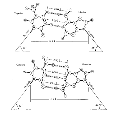
Figure 4: The nucleotide base-pairing in DNA with hydrogen bonds [22].

6.2 A physical scenario

The execution of the quantum search algorithm requires three ingredients: an interaction providing the quantum oracle $U_{b}$, a mechanism to generate the superposition state $|s\rangle$, and an environment where quantum coherence can survive. Let us look at how these may be realised in the case of DNA.

The formation of a molecular bond is a quantum process. Two reactants come together in an excited state, and the combined system decays to the bound state with the emission of an energy quantum. The total energy is conserved in the process, but the quantum dynamics of the transition between the two molecular energy levels alters the phase of the quantum state by $\sqrt{-1}$. This phase is a geometric phase, independent of the strength of the transition interaction and the time for the decay.

The DNA molecule is a double helix, and is often schematically represented as a ladder. The sides of the ladder have a periodic structure made of alternating sugar and phosphate groups, while the rungs of the ladder are made of paired nucleotide bases. The atomic structure of paired nucleotide bases is shown in Fig.4. The nucleotide bases are made of planar rings of atoms, and so the base-pairing requires at least two points of contact for structural stability of the helix (otherwise the bases would rotate relative to each other). The contacts between nucleotide bases are hydrogen bonds, which are formed by the quantum process of a proton tunneling between two attractive energy minima. When the nucleotide bases come together with arbitrary initial orientations, the base-pairing is likely to occur as a two step process—the first contact connects the two nucleotide bases and the second one locks their relative orientations. With such a two step base-pairing, the quantum state is transformed precisely by the operator $U_{b}$, i.e. the quantum state changes its sign when the nucleotide bases get paired and it remains unaffected when there is no pairing. From the known binding energy of the hydrogen bond and the uncertainty principle, the time scale for base-pairing can be estimated to be, $t_{b}\sim 10^{-14}$ sec.

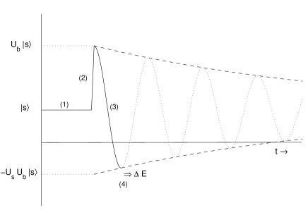
Figure 5: A time evolution scenario for the DNA replication process. Numerical labels refer to the steps described in Fig.3.

The quantum algorithm starts with the superposition state $|s\rangle$, so $|s\rangle$ has to be a stable equilibrium state. Any other initial state has to relax towards $|s\rangle$, and let $t_{r}$ be the time scale for this relaxation process. In case of DNA, $|s\rangle$ is a superposition state of chemically distinct nucleotide bases; it can be created only if the environment provides transition matrix elements between its various components. The nucleotide bases differ from each other by 5-10 atoms, and the transition matrix elements between them vanish in free space. Exchange of atomic groups is routine in chemical reactions, however—these reactions take place not with fixed number of atoms but with fixed chemical potential where exchange of atoms with the environment is allowed. (It is important to note that chemical reactions produce mixtures in classical environments while they produce superpositions in quantum environments.) The magnitudes of the transition matrix elements decide the speed at which $|s\rangle$ cycles through its various components. Let $t_{osc}$ be the time scale for these oscillations.

As illustrated in Fig.5, the quantum search algorithm can be executed when the above defined time scales satisfy the hierarchy,

$$t_{b}<<t_{osc}<<t_{r}~{}.$$ (8)

Explicitly, (1) the environment relaxes the initial state to $|s\rangle$, (2) the sudden base-pairing changes the state to $U_{b}|s\rangle$ (the energy quantum is not released yet), (3) the relaxation process tries to bring the state back to $|s\rangle$ causing damped oscillations, and (4) the energy quantum becomes free to wander off at the opposite end of oscillation; its irreversible release confirms the base-pairing and stops the search algorithm, $-U_{s}U_{b}|s\rangle=|b\rangle$.

This scenario is quite robust, and does not rely on fine-tuned parameters. The all important remaining question is whether the environment of DNA really has the properties ascribed to it, i.e. can it protect quantum coherence for a long enough time and create superposition states?

6.3 Decoherence and enzymes

High precision experiments have shown that quantum dynamics is the only valid description of the happenings at the atomic scale. Nevertheless, we hardly observe quantum effects in macroscopic systems; we find that macroscopic systems follow the quite different rules of classical dynamics. It cannot be discounted that the cross-over in the behaviour of physical systems is caused by some new laws of physics, as yet undiscovered. On the other hand, by a careful analysis of quantum dynamics, it is possible to explain the cross-over in a self-consistent manner. This explanation is labeled decoherence. It is a consequence of the fact that no quantum system is perfectly isolated; its inevitable interactions with its environment lead to irreversible loss of information and classical behaviour [25]. Irrespective of any undiscovered laws of physics, therefore, decoherence must be controlled in order to observe quantum effects (e.g. in quantum computers).

It is impossible to give a complete quantitative description of decoherence, because sufficient details of the environment are not available in general. Still we can construct a formulation good enough to provide order-of-magnitude estimates. The dominant interactions of a system with its environment are molecular collisions and long range forces. The cross-sections for these processes can be calculated in terms of global properties of the environment, such as temperature and density. Then the rate at which the system relaxes towards the equilibrium state favoured by the environment is estimated according to Fermi’s golden rule. (This relaxation is often referred to as the “collapse of the quantum wavefunction”.) The relaxation rate is inversely proportional to three factors: the initial flux, the interaction strength and the final density of states. Typical decoherence times are extremely short, beyond direct observation. But we also know specific situations, where quantum states are long-lived due to suppression of one or more of these factors. For instance, low temperatures and shielding reduce the initial flux, the interaction strength is small for lasers and nuclear spins, and the final density of states is suppressed for superconductors and hydrogen bonds due to energy gap.

It must be noted that the relaxation rate cannot become arbitrarily small when these factors become large. It is well-known that classical waves cannot be damped faster than the critical rate of damping, given by their natural period of oscillation. If the damping is increased beyond the critical value, the system stops relaxing instead of relaxing faster. The quantum analogue of this is the Zeno effect, which points out that a continuously monitored system cannot decay. The reason behind this caveat is that Fermi’s golden rule is an approximation, not valid at times smaller than the natural oscillation period. It follows that, in the notation of the previous subsection, $t_{osc}\leq t_{r}$ [26].

Biochemical reactions take place in a liquid medium at room temperature. In this environment, the decoherence times estimated following conventional thermodynamics and Fermi’s golden rule are miniscule. On the other hand, it is known that highly specific enzymes enhance the rates of biochemical reactions by orders of magnitude (as large as $10^{12}$) compared to estimates of kinetic theory and diffusion processes. Enzymes are catalysts, and the standard explanation of their properties is that they speed up the reactions by binding to the transition states and lowering the reaction barriers [27]. What the transition states are and how the reaction barriers are lowered must be explained ultimately in terms of underlying physical laws. A transition state is something in between the reactants and the products, which can be represented by distorted quantum wavefunctions, i.e. a superposition. The intermediate transition state will not be stable on its own, but the enzymes are able to store and supply free energy necessary for stabilising it. The reduction of reaction barrier by stabilisation of superposition states can provide a large speed up, because the tunneling amplitudes depend exponentially on the barrier size. Thus it is entirely possible that the enzymes perform their job by exploiting the quantum superposition phenomenon.

DNA replication takes place only in the presence of polymerase enzymes, so we must focus on the kind of environment they provide. The polymerase enzymes are much larger than the nucleotide bases, and they completely enclose the reaction region during replication. This behaviour automatically shields the reaction from the flux of external disturbances and reduces the final density of states by limiting possible configurations (the allowed phase space is essentially one-dimensional and not three-dimensional). The hydrogen bonds also reduce the final density of states, since their binding energy ($\sim 7kT$) is considerably larger than the thermal fluctuations. The polymerase enzymes drive the replication process monotonically, using free energy from ATP molecules, which is another indication that the thermal fluctuations are overcome.

Altogether, it is not inconceivable for a cleverly designed polymerase enzyme to create superposition states and protect quantum coherence in accordance with Eq.(8). Moreover, certain aspects of the quantum replication algorithm can be tested experimentally: artificial DNA with varying number of nucleotide bases can show whether 4 is the optimal number of nucleotide bases or not, and isotopic tagging can track whether superposition of atoms takes place or not [28].

7 Outlook

Information theory provides a powerful framework for extracting essential features of complicated processes of life, and then analysing them in a systematic manner. The easiest processes to study are no doubt the ones at the lowest level. We have learnt a lot, both in computer science and in molecular biology, since their early days [1, 29, 10], and so we can now perform a much more detailed analysis. Physical theories often start out as effective theories, where the predictions of the theories depend on certain parameters. The values of the parameters have to be either assumed or taken from experiments; the effective theory cannot predict them. To understand why the parameters have the values they do, we have to go one level deeper—typically to smaller scales, e.g. viscosity of fluids and crystal shapes of solids can be understood based on atomic forces, structure of atoms can be understood based on properties of electrons and quarks, and so on. When the deeper level reduces the number of unknown parameters, we consider the theory to be more complete and satisfactory. The level below conventional molecular biology is spanned by atomic structure and quantum dynamics, and that is the natural place to look for reasons behind life’s “frozen accident”. It is indeed wonderful that sufficient ingredients exist at this deeper level to explain the frozen accident as the optimal solution.

Counting the number of building blocks in the languages of DNA and proteins is only the first step. The obvious next step to investigate is why the languages use only the observed building blocks and not other similar ones; only a subset of nucleotide bases and amino acids existing in living cells are used as the building blocks. The likely criteria for the selection of particular building blocks are simplicity (for easy availability and quick synthesis) and functional ability (for implementing the desired tasks). In case of proteins, the choices are connected to the solution of the protein folding problem, i.e. which way a particular amino acid sequence will fold. In case of DNA, the choices are possibly connected with the magnitudes of the transition matrix elements. We do not have the answers yet, but we may not have to wait very long. The experimental techniques and the information collected in databases have reached a stage, where it is possible to form hypotheses and then test them. It would certainly be worthwhile to test the arguments presented here in detail, and then build on them to understand more and more complicated processes of life.

The results described here also allow us to speculate about the origin of life. All the complicated processes of life did not come about in one go. The lowest level of information processing not only arose first, but in all likelihood it was much simpler than what exists today. Importance of functionality over memory would put proteins before DNA. Similar codons for similar amino acids and wobble rules found in the present genetic code are possible relics of an earlier simpler system [30]. The solutions of the quantum search algorithm and the amino acid classes suggest that the present triplet genetic code was preceded by a doublet one. (This idea is reinforced by the accidental degeneracy, where 20 amino acids can be coded either by one classical and two quantum queries or by three quantum queries.) A still simpler precursor to the doublet code would be a singlet code of 4 amino acids. In fact such an evolutionary route for the genetic code has been proposed, just based on the chemical properties of the amino acids, GNC $\rightarrow$ SNS $\rightarrow$ NNN [31].

Unraveling the mysteries of life is certainly exciting. It is not merely a theoretical adventure; it has immense potential applications. Medical science will obviously benefit if we learn how to control processes of life that go wrong. Nanotechnology would benefit as well if we learn from biology how to implement specific tasks at the molecular scale.

References

- [1] One of the most influential work in this direction is: E. Schrödinger, What is life?, Cambridge university press, Cambridge (1944).
- [2] See for example: R. Dawkins, The selfish gene, Oxford university press, Oxford (1989).
- [3] Compared to deciphering an undocumented compiler written by someone else, it is much easier to write one’s own compiler from scratch, as anyone who has struggled with such problems would testify.
- [4] “Orthogonal transformations” have been enclosed in quotes here because it is the linear norm of the vector that is conserved. In conventional physical applications, orthogonal transformations represent conservation of the quadratic norm.
- [5] See for example: M.A. Nielsen and I.L. Chuang, Quantum computation and quantum information, Cambridge university press, Cambridge (2000).
- [6] The general subject of “zero-sum games” has not been explored in detail. The same arguments can be applied in a variety of situations, and may run counter to ethical principles, e.g. capitalism will conquer socialism.
- [7] C.E. Shannon, Bell System Tech. J. 27 (1948) 379; 623.
- [8] We don’t need exact value of in practical applications of geometry. We can first choose the desired accuracy of the result, and then find an appropriate digital approximation to to get the result within those bounds.
- [9] Written English is non-phonetic and does not make efficient use of its alphabet (e.g. “q” is always followed by “u”, even when new words like “qubit” are invented). But it will be a while before we come up with a more efficient alternative.
- [10] F.H.C. Crick, J. Mol. Biol. 38 (1968) 367.
- [11] A. Patel, J. Biosc. 27 (2002) 207, quant-ph/0103017.
- [12] The position of a point in a multi-dimensional space is often specified using orthogonal Cartesian coordinate system, i.e. a direct product of 1-dimensional coordinates. While there is nothing wrong with such a description, it is not the simplest choice.
- [13] The nitrogen atom of the peptide bond carries a positive charge, however, which makes its electronic behaviour similar to the tetravalent carbon atom.
- [14] G.N. Ramachandran, C. Ramakrishnan and V. Sasisekharan, J. Mol. Biol. 7 (1963) 95.
- [15] The smallest amino acid (glycine) is achiral, with hydrogen atom as the R-group. All the others are naturally found in the chiral L-type configurations, with the smallest among them (alanine) only rarely displaying the D-type configuration. Detailed model building studies have shown that all the R-groups in a polypeptide chain must be of the same chirality for the stability of regular secondary structures (-helices and -sheets).
- [16] J.G. Arnez and D. Moras, Trends Biochem. Sci. 22 (1997) 211.
- [17] B. Lewin, Genes VII, Oxford University Press, Oxford (2000).
- [18] There is one special amino acid in each class, involved in transformations beyond folding the backbone. Cysteine of class I forms long distance disulfide bonds, and proline of class I helps in “trans-cis” switch.
- [19] A. Patel, Proceedings of the Winter Institute on Foundations of Quantum Theory and Quantum Optics, Calcutta (2000), Pramāṇa 56 (2001) 367, quant-ph/0002037.
- [20] L.K. Grover, Proceedings of the 28th Annual ACM Symposium on Theory of Computing, Philadelphia (1996), p.212, quant-ph/9605043.
- [21] L.K. Grover and A. Sengupta, in Mathematics of quantum computation, R.K. Brylinski and G. Chen (eds.), CRC press (2002).
- [22] J.D. Watson, N.H. Hopkins, J.W. Roberts, J.A. Steitz and A.M. Weiner, Molecular biology of the gene, Fourth Edition, Benjamin/Cummings, Menlo Park (1987).
- [23] The number of ways items can be selected from a database containing multiple copies of 4 letters, , also gives for . This counting follows Bose statistics, i.e. it does not distinguish permutations. This and other elaborate combinatoric schemes were constructed to explain the number of amino acids, given that there are 4 nucleotide bases, but they fell apart with the discovery of the actual non-overlapping triplet genetic code (it does not possess permutation symmetry). For a recent summary of these efforts, see: B. Hayes, Am. Sci. 86 (1998) 8.
- [24] The solution is exact, and DNA replication is known to be quite error-free. The solutions for are not exact. They correspond to an error rate of about 1 part in 1000, which is not in conflict with the observed error rate in protein synthesis.
- [25] See for example: D. Giulini, E. Joos, C. Kiefer, J. Kupsch, I.-O. Stamatescu and H.D. Zeh, Decoherence and the appearance of a classical world in quantum theory, Springer, Berlin (1996).
- [26] See for example: T. Petrosky and V. Barsegov, in The chaotic universe, World Scientific, Singapore (2000).
- [27] See for example: A.L. Lehninger, D.L. Nelson and M.M. Cox, Principles of biochemistry, Second edition, Worth Publishers, USA (1993).
- [28] A. Patel, J. Genet. 80 (2001) 39, quant-ph/0102034.
- [29] J. von Neumann, The computer and the brain, Yale university press, New Haven (1958).
- [30] F.H.C. Crick, J. Mol. Biol. 19 (1966) 548.
- [31] K. Ikehara, Y. Omori, R. Arai and A. Hirose, J. Mol. Evol. 54 (2002) 530.