Rate equation theory of sub-Poissonian laser light

Abstract

Lasers essentially consist of single-mode optical cavities containing two-level atoms with a supply of energy called the pump and a sink of energy, perhaps an optical detector. The latter converts the light energy into a sequence of electrical pulses corresponding to photo-detection events. It was predicted in 1984 on the basis of Quantum Optics and verified experimentally shortly thereafter that when the pump is non-fluctuating the emitted light does not fluctuate much. Precisely, this means that the variance of the number of photo-detection events observed over a sufficiently long period of time is much smaller than the average number of events. Light having that property is said to be “sub-Poissonian”. The theory presented rests on the concept introduced by Einstein around 1905, asserting that matter may exchange energy with a wave at angular frequency $\omega$ only by multiples of $\hbar\omega$. The optical field energy may only vary by integral multiples of $\hbar\omega$ as a result of matter quantization and conservation of energy. A number of important results relating to isolated optical cavities containing two-level atoms are first established on the basis of the laws of Statistical Mechanics. Next, the laser system with a pump and an absorber of radiation is treated. The expression of the photo-current spectral density found in that manner coincides with the Quantum Optics result. The concepts employed in this paper are intuitive and the algebra is elementary. The paper supplements a previous tutorial paper [Arnaud (1995)] in establishing a connection between the theory of laser noise and Statistical Mechanics.

42.55.Ah, 42.50.Ar, 42.55.Px, 42.50.Lc

1 Introduction

The purpose of this paper is to present a derivation of the essential formulas relating to sub-Poissonian light generation in a simple and self-contained manner. This is done on the basis of a theory in which the light field enters through its energy. Only single-mode cavities incorporating emitting and absorbing atoms are considered. Some Quantum-Optics effects [Elk (1996)] that become inconspicuous when the number of atoms is large are neglected. The paper does not assume specialized knowledge from the reader, but some understanding of general concepts relating to random variables (mean, variance) and stationary random functions of time (spectral densities) [Papoulis (1965)], may be useful.

Laser light possesses high degrees of directivity and monochromaticity. The intensity fluctuations, though relatively small, are of practical significance in some applications: transmission of information by means of optical pulses, measurement of small attenuations, or interferometric detection of gravitational waves. Lasers essentially consist of single-mode optical cavities containing resonant atoms with a supply of energy called the pump and a sink of energy, presently viewed as an optical detector (see Figure 1). The latter converts light into a series of identical electrical pulses, referred to as “photo-detection events” [Koczyk et al. (1996)]. If the events are independent of one another, the light impinging on the detector is said to be “Poissonian”, and the photo-current fluctuations are at the “shot-noise level”. But under some circumstances detection events occur more regularly, in which case the light is said to be “sub-Poissonian”. Light of that nature has been first observed by short. Subsequently, yamamoto performed a remarkable series of experiments on laser diodes. They observed a reduction by up to a factor of 10 below the shot-noise level. The correlation between the number of upper-state atoms in the cavity and photo-detection events has also been measured [Richardson and Yamamoto (1991)].

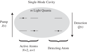
Figure 1: Schematic representation of a laser. The single-mode cavity (shown as a gray oval) incorporates active two-level atoms (only two are shown on the left, one in the upper state and one in the lower state) and absorbing (detecting) atoms (only one is shown on the right). The pump raises active atoms from their lower to upper states at some prescribed rate $\mathcal{J}$. Photo-detection events occur at rate $\mathcal{Q}$. At low frequencies, ${\mathcal{Q}}(t)={\mathcal{J}}(t)$.

A single-mode optical cavity resonating at angular frequency $\omega$ may be modeled as an inductance-capacitance ($L,C$) circuit with $LC\omega^{2}=1$. The active atoms, located between the capacitor plates, interact with a spatially uniform optical field through their electric dipole moment (see, for example, milonni). In this idealized model, the field angular frequency “seen” by the atoms is equal to $\omega$ In the present idealized model, no momentum is transfered between the field and the atoms, so that the Maxwellian atomic-velocity distribution is undisturbed. An advanced relativistic treatment can be found in benyaacov.. The 2-level atoms (with the lower level labeled “1” and the upper level labeled “2”) are supposed in this paper to be resonant with the field. This means that the atomic levels 1 and 2 are separated in energy by $\hbar\omega$, where $\hbar$ denotes the Planck constant divided by $2\pi$. The energy unit is taken equal to $\hbar\omega$, for simplicity. The pumping rate $\mathcal{J}$, defined as the number of atoms raised to their upper state per unit time, is supposed to be a prescribed function of time, i.e., to be independent of the laser dynamics. This condition is actually achieved in the case of semiconductors with the help of high-impedance electrical sources. It has been shown further [Khazanov et al. (1990), Ritsch et al. (1991), Ralph and Savage (1993)] that sub-Poissonian output light statistics should be obtainable also from four-level atom lasers with incoherent optical pumping In the case of 4-level atom lasers (with levels labeled from 0 to 3, the working levels being those labeled 1 and 2), strong optical pumping resonant with levels 0 and 3 provides a constant probability that electrons in level 0 be transfered to level 3 per unit time, and (almost) the same probability that electrons in level 3 be transfered to level 0. The detected-light fluctuations may be sub-Poissonian at zero baseband frequency. Precisely, the spectral density is half the shot-noise level under ideal conditions (negligible spontaneous decay, negligible optical loss, and quick decay from level 3 to level 2). This desirable behavior results from level 0 population fluctuations.. This important observation escaped the attention of previous laser theorists. For such four-level lasers the expressions obtained from the present theory are identical to those reported in these references [Chusseau and Arnaud (2001)]. The output light fluctuates at only one third of the shot-noise level.

The light-energy absorber is modeled as an ideal optical detector that generates a series of identical electrical pulses, the energy lost by the field being entirely dissipated in the detector load. Unlike active atoms, detector atoms remain most of the time in the ground state, with quick non-radiative decay after an excitation event. For the sake of conceptual clarity, the absorber of radiation is supposed to be located within the optical cavity as in the sargent classical text-book In our model, detection (linear absorption) is supposed for the sake of simplicity to occur within the optical cavity. But no difference of behavior is observed when a laser beam is absorbed externally without reflection, rather than internally, at the same average rate. It is therefore expected that the present theory be applicable to reflectionless external detectors. In open-space configurations, legitimate questions could be raised in connection with the law of causality. It is therefore important to emphasize that only single-mode cavities are considered in the present paper, and that the concept of propagating light is not relevant. Note further that the theory would hold just as well if the optical resonator were replaced, for example, by an acoustical resonator at the same frequency. The wave is localized, and its physical nature is unimportant.. The main purpose of this paper is to derive an expression of the photo-current spectral density, particularly in the limit of small Fourier (or “baseband”) frequencies In Optical Communications, $\Omega$ is often called “baseband” angular frequency and $\omega$ “carrier” angular frequency. It is a common practice to consider only positive baseband frequencies, so that factors of 2 may arise as one goes from the Physics to the Engineering literature. The time dependence at baseband frequencies is denoted in this paper by: exp$(j\Omega t)$. To define the photocurrent spectral density, consider a particular (experimental or computer-generated) run lasting from $t=0$ to $\tau_{m}$, the photodetection events occurring at times $t_{1},t_{2},\ldots,t_{i},\ldots$. The detection rate ${\mathcal{Q}}(t)$ is defined as the sum over $i$ of $\delta(t-t_{i})$, where $\delta(.)$ denotes the Dirac distribution. The detector electrical current, if desired, would be obtained by multiplying ${\mathcal{Q}}(t)$ by $e$, the absolute value of the electron electrical charge. The (real, nonnegative) spectral density $S_{\Delta Q}(\Omega)$ of $\Delta Q\equiv Q(t)-\left\langle{Q}\right\rangle$ is defined as: $\left\langle{\left|{\sum\exp(j\Omega t_{i})}\right|^{2}}\right\rangle/\tau_{m}$ , where brackets denote an average over many runs, and $\Omega=2\pi n/\tau_{m}$, with $n=1,2\ldots$. This expression is accurate if the measurement time $\tau_{m}$ is sufficiently large. In the special case where the photo-detection events are independent of one another, and uniformly distributed (uniform Poisson process), we have $S_{\Delta Q}(\Omega)=\left\langle{Q}\right\rangle$, a relation usually referred to as the “shot-noise formula”. The variance of the number of events occurring during some time T is in that case equal to the average number of events, see Eq. (5.37) of [Papoulis (1965)]..

Consider now some theories of sub-Poissonian light generation. The main concept of Quantum Optics, introduced by Dirac in 1927, is that the field in a cavity should be treated as a quantized harmonic oscillator. Following Dirac’s lead, laser theorists, initially, were mostly concerned with the state of the cavity field. But Golubev and Sokolov, in 1984, carefully distinguished the fluctuations of the field in the cavity from those of the detection rate. They further pointed out that when lasers are driven by non-fluctuating pumps, the emitted light should be sub-Poissonian. Similar results were subsequently obtained by yamamoto, see also Meystre and Walls (1991); Walls and Milburn (1994); Davidovitch (1996); Mandel and Wolf (1995). These authors employed various approximations of the laws of Quantum Optics, and various models to describe non-fluctuating pumps. No approximation is made in the recent numerical work of elk. But because the computing time grows exponentially with the number of atoms present in the cavity, the author is able to give results only for up to 5 atoms. Even with few atoms, some typical features of Quantum Optics (the so-called trapped states) get washed out, so that simplified theories may be adequate. loudon and jakeman have treated the evolution in time of the number of photons in a laser amplifier on the basis of a theory in which the optical field is not explicitly quantized, as is done here. Such theories are able to describe sub-Poissonian light when the detecting atoms are included in the system description [3]. Accurate noise sources have been obtained by Gordon in 1967 (see Section 5 of gordon entitled “The generalized Wigner density and the approximate classical model”) through symmetrical ordering of operators. Gordon did not address, however, the case of non-fluctuating pumps. Application of the Gordon formalism to non-fluctuating-pump lasers was made independently in 1987-88 by katanaev and this author Arnaud (1988). A discussion is given by nilsson.

Theories in which the atoms are quantized but the optical field is not directly quantized are usually labeled “semiclassical”. However, because this adjective may cause confusion with alternative theories Many authors attempted to avoid the intricacies of field-quantization. But while there is essentially only one quantum theory, there exist many distinct theories in which the field is treated in a classical manner. When the operators entering in the exact Quantum Optics theory are normally ordered, linearized, and the operator character of the field is ignored, a theory emerges called in the Optical-Engineering literature the “phasor” theory. According to that theory, quantum noise would be caused by the field spontaneously emitted by atoms in the excited state. But a detailed comparison (see Appendix B of arnaudIEEJ) shows that the phasor theory, though plausible on some respects, is unable to explain the origin of sub-Poissonian light. On the other hand, funk, raymer, and savage, note that “The observed sub-Poissonian statistics are unexplainable using classical and semi-classical theories”. This statement applies to the usual semiclassical theories in which the absorber is forbidden to react on the field. But a key point of the present theory is that absorbers do react on the field. The observation that “Sub-Poissonian statistics are possible only for a non-classical field” Mandel and Wolf (1995) is meaningful in the context of Quantum Optics, but not in the context of the present theory since the “state” of the field (in the Quantum Optics sense) is not considered. the present theory has been called simply: “classical”, to emphasize that the light field enters only through its energy, a classical quantity. But the reader is warned that the theory is not strictly classical. Randomness enters because the atomic transitions obey a probability law rather than a deterministic law. Note also that the expression rate equation employed in the title sometimes refer to the time evolution of average quantities, and random fluctuations are ignored. In this paper, the expression rate equation is understood in a broader sense as, e.g., in the paper by ralph.

The theory presented rests first of all on the concept introduced by Einstein early in the previous century asserting that matter may exchange energy with a wave at angular frequency $\omega$ only by multiples of $\hbar\omega$ Kuhn (1987). The law of energy conservation in isolated systems entails that, if the matter energy is quantized, the field energy may only vary by integral multiples of $\hbar\omega$. Thus, no independent degree of freedom is ascribed to the field. This is in sharp contrast with the Quantum Optics view-point. The physical picture that emerges from the present theory is that laser-light fluctuations are caused by the random stimulated transitions responsible for light emission and absorption During a jump from one state to another, an atom is in a state of superposition. But such states need not be considered explicitly as only global conservation laws are being employed (quantum jumps are discussed, e.g., in greenstein). Likewise, the interaction energy that may exist during a jump needs not be considered explicitly.. If the number of atoms in the upper state is denoted by $n$ and the number of light quanta The word “photon” suggesting that light consists of tiny particles moving in space should better be avoided in the context of this paper, see the interesting paper by lamb. in the cavity by $m$, $n+m$ is a conserved quantity in isolated systems. It may vary only in response to the pump generation rate or the detector absorption rate.

The paper is organized as follows. It is first observed in Section 2 that useful information on laser light may be obtained by considering isolated optical cavities containing atoms in a state of equilibrium, and using the methods of Statistical Mechanics (for an introduction to that field, see for instance Schroeder (1999)).

When the total system (matter$+$field) energy is sufficiently large, the equilibrium state is highly non-thermal. In fact, the gain saturation mechanism that characterizes laser operation is as work in the isolated system as well: whenever the light intensity exceeds its average value there is a decrease of the number of atoms in the excited state (through energy conservation), and therefore a reduction of the total probability that a stimulated emission event will occur within the next elementary time interval. This effect prevents the light intensity from varying much. The great interest of the laws of Statistical Mechanics is that they provide important informations about the equilibrium state without having to consider in detail how the system evolves in the course of time. Precisely, we find that the variance of the number of light quanta in the cavity is half the average number of quanta, that is, the field statistics is sub-Poissonian. This result is of direct practical significance if the light energy contained in the cavity is allowed to radiate into free-space at some instant. The emitted light pulse is indeed sub-Poissonian, though not fully “quiet”.

In Section 3, the equilibrium situation enables us to recover the Einstein prescription asserting that the probability that electrons be promoted to upper levels is $Cm$ and the probability that they be demoted to lower levels is $C(m+1)$, where $m$ denotes the number of light quanta in the cavity and $C$ a constant proportional to the Einstein $B$-coefficient of stimulated emission and absorption. The equilibrium situation provides the rate at which light quanta would be absorbed at high Fourier frequencies.

But, in order to obtain accurately the rate at any Fourier frequency, it is necessary to include explicitly pump fluctuations and the reaction of the absorbed rate on the field (see Section 4). An appendix clarifies the fact that, even though no entropy is ascribed to the field in the present theory, the isolated system entropy increases when some piece of matter is introduced into an initially empty cavity, as the second law of Thermodynamics requires. It is shown that the entropy that Quantum Optics ascribes to single-mode fields is the difference between the system entropy and the average matter entropy.

2 Isolated cavities in a state of equilibrium

Consider $N$ identical two-level atoms. For each atom, the zero of energy is taken at the lower level and the unit of energy at the upper level (typically, 1 eV). The atoms are supposed to be coupled to one another so that they reach a state of equilibrium before other parameters have changed significantly. The strength of the atom-atom coupling, however, needs not be specified further. The atoms are supposed to be at any time in either the upper or lower state. The number of atoms that are in the upper state is denoted by $n$, and the number of atoms in the lower level is therefore $N-n$. According to our conventions, the atomic energy is equal to $n$. Its maximum value $N$ occurs when all the atoms are in the upper state. There is population inversion when the atomic energy $n>N/2$.

The statistical weight $W(n)$ of the atomic collection is the number of distinguishable configurations corresponding to some total energy $n$. For two atoms ($N=2$), for example, $W(0)=W(2)=1$ because there is only one possible configuration when both atoms are in the lower state $(n=0)$, or when both are in the upper state $(n=2)$. But $W(1)=2$ because the energy $n=1$ obtains with either one of the two (distinguishable) atoms in the upper state. For $N$ identical atoms, the statistical weight (number of ways of picking up $n$ atoms out of $N$) is (see papoulis, p. 58)

$$W(n)=\frac{N!}{n!(N-n)!}.$$ (1)

Note that $W(0)=W(N)=1$ and that $W(n)$ reaches its maximum value at $n=N/2$ (supposing $N$ even), with $W(N/2)$ approximately equal to $2^{N}\sqrt{2/\pi N}$. Note further that

$$Z\equiv\sum_{n=0}^{N}W(n)=2^{N}.$$ (2)

Consider next an isolated single-mode optical cavity (see Figure 1 without the pump and the detector), containing $N$ resonant two-level atoms. The atoms perform jumps from one state to another in response to the optical field so that the number of atoms in the upper state is a function $n(t)$ of time. If $m(t)$ denote the number of light quanta at time $t$, the sum $n(t)+m(t)$ is a conserved quantity (essentially the total atom+field energy). Thus, $m$ jumps to $m-1$ when an atom in the lower state gets promoted to the upper state, and to $m+1$ in the opposite situation. If $N$ atoms in their upper state are introduced at $t=0$ into the empty cavity ($m=0$), part of the atomic energy gets converted into field energy as a result of the atom-field coupling and eventually an equilibrium situation is reached. The basic principle of Statistical Mechanics asserts that all states of isolated systems are equally likely. Accordingly, the probability $P(m)$ that some $m$ value occurs at equilibrium is proportional to $W(N-m)$, where $W(n)$ is the statistical weight of the atomic system defined in (1) (see Appendix B of arnaudAJP). As an example, consider two (distinguishable) atoms ($N$=2). A microstate of the isolated (matter$+$field) system is specified by telling whether the first and second atoms are in their upper (1) or lower (0) states and the value of $m$. Since the total energy is $N=2$, the complete collection of microstates (first atom state, second atom state, field energy), is: (1,1,0), (1,0,1), (0,1,1) and (0,0,2). Since these four microstates are equally likely, the probability that $m=0$ is proportional to 1, the probability that $m=1$ is proportional to 2, and the probability that $m=2$ is proportional to 1. This is in agreement with the fact stated earlier that $P(m)$ is proportional to $W(N-m)$. After normalization, we obtain for example that P(0)=1/4.

The normalized probability reads in general

$$P(m)=\frac{W(N-m)}{Z}=\frac{N!}{2^{N}m!(N-m)!}.$$ (3)

It is shown in the Appendix that the system entropy $S(t)$ increases from $S(0)=\ln[W(N)]=0$ at the initial time ($m=0,n=N$), to $S(\infty)=\ln[Z]=N\ln(2)$ when the equilibrium state has been reached. Note that no entropy is ascribed to single-mode fields, as they are fully characterized by their energy. The moments of $m$ are defined as usual as

$$\left\langle{m^{r}}\right\rangle\equiv\sum_{m=0}^{N}m^{r}P(m),$$ (4)

where brackets denote averagings. It is easily shown from (3), (4) that $\left\langle{m}\right\rangle=N/2$ and $\mathrm{var}(m)\equiv{\left\langle{m^{2}}\right\rangle-\left\langle{m}\right\rangle^{2}}=N/4$. Thus the number $m$ of light quanta in the cavity fluctuates, but the statistics of $m$ is sub-Poissonian, with a variance less than the mean.

The expression of $P(m)$ in (3) just obtained has physical and practical implications. Suppose indeed that the equilibrium cavity field is allowed to escape into free space, thereby generating an optical pulse containing $m$ quanta. It may happen, however, that no pulse is emitted when one is expected, causing a counting error. From the expression in (3) and the fact that $\left\langle{m}\right\rangle=N/2$, the probability that no quanta be emitted is seen to be $P(0)=4^{-\left\langle{m}\right\rangle}$. For example, if the average number of light quanta $\left\langle{m}\right\rangle$ is equal to $20$, the communication system suffers from one counting error (no pulse received when one is expected) on the average over approximately $10^{12}$ pulses. Light pulses of equal energy with Poissonian statistics are inferior to the light presently considered in that one counting error is recorded on the average over $\exp(\left\langle{m}\right\rangle)=\exp(20)\approx 0.5~{}10^{9}$ pulses (see, for example, p. 276 of milonni).

3 Time evolution of the number of light quanta in isolated cavities

Let us now evaluate the probability $P(m,t)$ that the number of light quanta be $m$ at time $t$. Note that here $m$ and $t$ represent two independent variables. A particular realization of the process was denoted earlier $m(t)$. It is hoped that this simplified notation will not cause confusion.

Let $E(m)dt$ denote the probability that, given that the number of light quanta is $m$ at time $t$, this number jumps to $m+1$ during the infinitesimal time interval [$t,t+dt$], and let $A(m)dt$ denote the probability that $m$ jumps to $m-1$ during that same time interval (the letters “$E$” and “$A$” stand respectively for “emission” and “absorption”). $P(m,t)$ obeys the relation

$$P(m,t+dt) = P(m+1,t)A(m+1)dt$$ (5)

$$+P(m-1,t)E(m-1)dt$$

$$+P(m,t)\left(1-A(m)dt-E(m)dt\right).$$

Indeed, the probability of having $m$ quanta at time $t+dt$ is the sum of the probabilities that this occurs via states $m+1$, $m-1$ or $m$ at time $t$. All other possible states are two or more jumps away from $m$ and thus contribute negligibly in the small $dt$ limit (see gillespie, p. 381). After a sufficiently long time, one expects $P(m,t)$ to be independent of time, that is: $P(m,t+dt)=P(m,t)\equiv{P(m)}$. It is easy to see that (5) satisfies this condition if

$$P(m+1)A(m+1)=P(m)E(m).$$ (6)

This “detailed balancing” relation holds true because $m$ cannot go negative (see gillespie, p. 425). When the expression of $P(m)$ obtained in (3) is introduced in (6), one finds that

$$\frac{E(m)}{A(m+1)}=\frac{P(m+1)}{P(m)}=\frac{N-m}{m+1},$$ (7)

a relation that admits the solution

$$E(m)=(N-m)(m+1),\qquad A(m)=m^{2}.$$ (8)

It is natural to suppose that the probability $E$ of atomic decay is proportional to the number $n$ of atoms in the upper state, and that the probability $A$ of atomic promotion is proportional to the number $N-n$ of atoms in the lower state. Thus, we introduce the functions of two variables ($n,m$)

$$E(n,m)=n(m+1),\qquad A(n,m)=(N-n)m,$$ (9)

with the understanding that $E(m)=E(N-m,m)$ and $A(m)=A(N-m,m)$. These relations hold within a proportionality factor. Setting this proportionality factor as unity amounts to fixing the time scale. The expressions in (9) say that the probability that an atom gets promoted to the upper level in the time interval $[t,t+dt]$ is equal to $mdt$, while the probability of atomic decay is $(m+1)dt$. These expressions were obtained by Einstein in 1917 in a somewhat different manner Assuming that the atoms emit or absorb a single light quantum at a time (“1-photon” process), the strictly-classical limit tells us that the probability that an atom in the upper state decays must be a linear function of $m$, i.e., we must have $E(n,m)=n(am+b)$, where $a,b$ and later $c,d$ are constants. Likewise, the probability of atomic promotion must be of the form: $A(m)=(N-n)(cm+d)$. But, furthermore, $A$ is required to vanish for $m=0$ since, otherwise, $m$ could go negative. Accordingly, $d=0$. Remembering that $n=N-m$, we find upon substitution of $E(m)=(N-m)(am+b)$ and $A(m)=mcm$ in the detailed-balancing relation and simplifying that: $am+b=cm+c$, a relation which is satisfied for all $m$ values only if $a=c$ (equality of stimulated emission and absorption coefficients), and $b=c=a$. To within a constant factor, we have therefore $E(n,m)=n(m+1)$, and $A(n,m)=(N-n)m$, relations discovered by Einstein at the turn of the previous century. Note that the “1” in the term $m+1$ of $E(n,m)$ is sometimes ascribed to spontaneous emission in the mode. The lack of symmetry between $m+1$ (emission) and $m$ (absorption) is only apparent. If indeed the field energy is defined as $m+1/2$, upward and downward transition probabilities may be both written as the arithmetic averages of the field energy before and after the jump..

Let us now restrict our attention to the steady-state regime and large values of $N$. Since $m$ is large, the “1” in the expression $m+1$ of $E(m)$ may be neglected. Furthermore, in that limit, $m$ may be viewed as a continuous function of time with a well-defined time-derivative. Because the standard deviation $\sqrt{N/4}$ of $m$ is much smaller than the average value, the so-called “weak-noise approximation” is permissible Gillespie (1992). Within that approximation, the average value $\left\langle{f(n,m)}\right\rangle$ of any smooth function $f(n,m)$ may be taken as approximately equal to $f(\left\langle{n}\right\rangle,\left\langle{m}\right\rangle)$.

The evolution in time of a particular realization $m(t)$ of the process obeys the classical Langevin equation

$$\frac{dm}{dt}=\mathcal{E}-\mathcal{A},$$ (10)

where

$${\mathcal{E}}\equiv E(m)+e(t),\qquad{\mathcal{A}}\equiv A(m)+a(t).$$ (11)

In these expressions, $e(t)$ and $a(t)$ represent uncorrelated white-noise processes whose spectral densities equal to $E\equiv E(\left\langle{m}\right\rangle)$ and $A\equiv A(\left\langle{m}\right\rangle)$, respectively A formal proof of the validity of the Langevin equation will not be given here. Instead, it will be shown that the variance of $m$ obtained from the Langevin equation coincide with the result obtained directly from Statistical Mechanics. Without the noise sources, the evolution of $m$ in (10) would be deterministic, with a time-derivative equals to the drift term $E(m)-A(m)$. If the expressions (8) are employed, the Langevin equation (10) reads

$$\frac{dm}{dt} = Nm-2m^{2}+e-a,$$

$$S_{e-a} = E+A=N\left\langle{m}\right\rangle=N^{2}/2,$$ (12)

where the approximation $N\gg 1$ has been made.

Let $m(t)$ be expressed as the sum of its average value $\left\langle{m}\right\rangle$ plus a small deviation $\Delta m(t)$, and $Nm-2m^{2}$ in (12) be expanded to first order. A Fourier transformation of $\Delta m(t)$ with respect to time amounts to replacing $d/dt$ by $j\Omega$ [4]. The Langevin equation now reads

$$j\Omega\Delta m=-N\Delta m+e-a,\qquad S_{e-a}=N^{2}/2,$$ (13)

where $m$ has been replaced by its average value $N/2$.

Since the spectral density of $z(t)=ax(t)$, where $a\equiv{a^{\prime}+ja^{\prime\prime}}$ is a complex number and $x(t)$ a stationary process, reads: $S_{z}(\Omega)=|a|^{2}S_{x}(\Omega)$, one finds from (13) that the spectral density of the $\Delta m(t)$ process is

$$S_{\Delta m}(\Omega)=\frac{N^{2}/2}{N^{2}+\Omega^{2}}.$$ (14)

The variance of $m$ is the integral of $S_{\Delta m}(\Omega)$ over frequency ($\Omega/2\pi$) from minus to plus infinity, that is: var$(m)=N/4$ in agreement with the previous result in Section 2.

Suppose now that a small absorbing body, perhaps a single atom that remains most of the time in its lower state as discussed earlier, is introduced in the cavity. One expects that this unique atom will not affect significantly the average value and the statistics of $m$ for some period of time. If $m$ were non-fluctuating, the probability that a detection event occurs during the time interval $[t,t+dt]$, divided by $dt$, would be a constant. This property defines the Poisson process. Since $m$ actually suffers from the fluctuations discussed earlier in this section, the detection rate is super-Poissonian, with a spectral density that exceeds the average detection rate.

The expression for the detection rate has the same form as the one introduced earlier for the stimulated absorption rate $A$, the only difference being that in the detector atoms remain in the lower state most of the time, as discussed in the introduction. Accordingly

$${\mathcal{Q}}=\alpha m+q,\qquad\Delta Q=\alpha\Delta m+q,$$ (15)

where $\alpha$ denotes a constant. The noise sources $e(t)$, $a(t)$, and $q(t)$ are uncorrelated white-noise processes of spectral densities $E$, $A$, and $Q\equiv\alpha\left\langle{m}\right\rangle$, respectively.

The spectral density of the detection rate fluctuation $\Delta Q$ defined in (15) may be obtained directly from (14) since $q(t)$ is presently supposed to be uncorrelated with the other noise sources

$$S_{\Delta Q}(\Omega)=\alpha^{2}S_{\Delta m}(\Omega)+Q=\alpha^{2}\frac{N^{2}/2}{N^{2}+\Omega^{2}}+Q.$$ (16)

Consideration of optical cavities close to a state of equilibrium therefore provides some information concerning the detection rate statistics. But the conclusion that the detection rate fluctuations always exceed the shot-noise level holds true only when $\Omega\gg\sqrt{\alpha N}$. After a sufficiently long time, even a single absorbing atom affects the statistics of $m$ in such a drastic way that the result in (16) becomes invalid. A true steady-state may be obtained only if a pumping mechanism compensates for the energy loss caused by light-quanta absorption. The accurate result, to be given next, shows that, at low frequencies, the detection rate depends in a crucial way on the pump fluctuations.

4 Laser noise

Lasers are open systems with a source of energy called the pump, and a sink of energy presently viewed as an ideal optical detector. It is natural to suppose that the probabilities of atomic decay or atomic promotion that were found earlier consistent with the laws of statistical mechanics, still hold when there is a supply of atoms in the upper state (the pump), and an absorber of light energy (the detector).

The evolution equation for the number $m$ of light quanta is thus obtained by subtracting the loss rate $\mathcal{Q}$ from the right-hand-side of (10). Since the system is not isolated, $n+m$ may now fluctuate, and the expressions of $E(n,m)$ and $A(n,m)$ given in (9) must be employed. A second equation describing the evolution of the number $n$ of atoms in the upper state is needed, which involves the prescribed pump rate ${\mathcal{J}}(t)$. To summarize, the evolution equations for $m$ and $n$ are

$$\frac{dm}{dt} = \mathcal{E}-\mathcal{A}-\mathcal{Q},$$ (17)

$$\frac{dn}{dt} = \mathcal{J}-\mathcal{E}+\mathcal{A},$$ (18)

where

$$\begin{array}[]{lll}{\mathcal{E}}\equiv E(n,m)+e(t),&E(n,m)=nm,&S_{e}=E,\\ {\mathcal{A}}\equiv A(n,m)+a(t),&A(n,m)=(N-n)m,&S_{a}=A,\\ {\mathcal{Q}}\equiv\alpha m+q(t),&&S_{q}=Q,\\ {\mathcal{J}}\equiv J+\Delta J(t).&&\end{array}$$ (19)

In the steady-state, the right-hand-sides of (17) and (18) vanish, and we have: $J=E-A=Q$, that is $J=(2\left\langle{n}\right\rangle-N)\left\langle{m}\right\rangle=\alpha\left\langle{m}\right\rangle$. Thus, $\left\langle{m}\right\rangle=J/\alpha$ and $2\left\langle{n}\right\rangle-N=\alpha$. This relation expresses the fact that the stimulated emission gain coefficient ($\left\langle{n}\right\rangle$) minus the stimulated absorption loss coefficient ($N-\left\langle{n}\right\rangle$) equals in the steady state the linear loss coefficient $\alpha$.

Next, observe that at small frequencies, the left-hand-sides of the previous equations (17) and (18) may be neglected. The simple relation ${\mathcal{Q}}(t)={\mathcal{J}}(t)$ follows, proving that the detection rate does not fluctuate (${\mathcal{Q}}=$constant) if the pump is non-fluctuating or “quiet” (${\mathcal{J}}=$constant). The relation ${\mathcal{Q}}(t)={\mathcal{J}}(t)$ holds at low frequencies even in the presence of internal conservative effects such as gain compression (due, for example, to spectral hole burning), gain guidance, or mesoscopic effects that occur when the thermal energy $k_{B}T$ is not large compared to the average level spacings Arnaud et al. (1999, 2000).

A quiet pump is henceforth assumed. When the above equations are linearized and $\Delta{m},\Delta{n}$ are Fourier transformed, one obtains

$$j\Omega\Delta m = 2\left\langle{m}\right\rangle\Delta n+e-a-q,$$ (20)

$$j\Omega\Delta n = -2\left\langle{m}\right\rangle\Delta n-\alpha\Delta m-e+a.$$ (21)

Let us recall that $e$, $a$ and $q$ are uncorrelated white-noise processes whose spectral densities are equal to the corresponding average rates. After elimination of $\Delta n$ from the above two equations, $\Delta m$ may be expressed in terms of uncorrelated noise sources

$$\Delta m=\frac{j\Omega(e-a)-(2\left\langle{m}\right\rangle+j\Omega)q}{j\Omega 2\left\langle{m}\right\rangle+\alpha 2\left\langle{m}\right\rangle-\Omega^{2}}.$$ (22)

We then proceed as in the previous section, evaluating the spectral density of $\Delta m$ and integrating over frequency to obtain the variance of $m$. The result is

$$\frac{\mathrm{var}(m)}{\left\langle{m}\right\rangle}=\frac{N+\alpha}{4\left\langle{m}\right\rangle}+\frac{1}{2}.$$ (23)

In the limit that $\alpha\ll N$ and $\left\langle{m}\right\rangle=N/2$, the right-hand-side of (23) is 1 while the corresponding result in Section 2 relating to the isolated cavity is 1/2. This is due to the singular behavior of the spectral density of $\Delta m$ at $\Omega=0$ in the limit considered. Physically, this means that small losses allow $m(t)$ to drift slowly.

We are mostly interested in the detection rate fluctuation $\Delta Q=\alpha\Delta m+q$. Notice that $m$ and $q$ are correlated. Proceeding as in the previous section, we obtain

$$\frac{S_{\Delta Q}(\Omega)}{Q}-1=\frac{\left((N+\alpha)/4\alpha\left\langle{m}\right\rangle^{2}\right)\Omega^{2}-1}{(\Omega/\alpha)^{2}+\left(1-\Omega^{2}/2\alpha\left\langle{m}\right\rangle\right)^{2}}.$$ (24)

In the limit that $\alpha\ll N$, $\left\langle{m}\right\rangle=N/2$, the above result reduces to the one given in Section 3 at high frequencies: $\Omega\gg\sqrt{\alpha N}$.

Comparison between the results in (16) and (24) is exemplified in Figure 2 for $N=100$, $\alpha=20$ and $m=N/2$. In the exact treatment, the spectral densities of the photodetection process go to zero at zero baseband (or Fourier) frequencies. Note also that, for the parameter values considered, a relaxation oscillation peak appears. In the large optical power limit ($\left\langle{m}\right\rangle\gg 1$), the above expression reduces to

$$\frac{S_{\Delta Q}(\Omega)}{Q}=1-\frac{1}{(\Omega/\alpha)^{2}+1}.$$ (25)

Expressions obtained from the present theory have invariably been found to coincide with the Quantum Optics results when the same approximations are made, essentially the large atom number approximation. In particular, the simple expression in (25) was first given by yamamoto, see Figure 15-10, b). The expression for the atomic-number detection-rate correlation was first obtained from a theory similar to the one described in the present paper Arnaud and Estéban (1990).

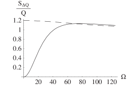
Figure 2: Normalized spectral density $S_{\Delta Q}(\Omega)/Q$ of the detection rate $\mathcal{Q}$ as a function of the normalized baseband (or Fourier) frequency $\Omega$. The number of atoms is $N=100$ and the cavity loss rate (due to the detection process) is $\alpha=20$. The average number of light quanta is $\left\langle{m}\right\rangle=N/2$. Plain lines: exact result from the discussion in Section 4. Dashed lines: approximate result for nearly isolated cavities, see Section 3.

5 Conclusion

The purpose of this paper was to show that, in the limit of a large number of atoms, important results relating to laser light fluctuations, usually derived on the basis of Quantum Optics, may be obtained in a much simpler manner. This is so even if the detected light statistics is sub-Poissonian. The light field enters only through its energy, which is quantized as a result of atomic quantization and conservation of energy but not directly.

For the sake of simplicity, many effects have been neglected. But the theory may be generalized to account for spontaneous carrier recombination, phase-amplitude coupling, and complicated cavity structures Siegman (1986, 1995). Besides the intensity noise, other useful quantities may be evaluated, particularly phase noise Arnaud (1988, 1997). When the atoms get close to one another, the upper and lower levels spread into bands called in the field of Semiconductor Physics, “conduction” and “valence” bands, with $k_{B}T$ small compared with the widths of the bands. In that situation the Fermi-Dirac distribution (see for example chusseau) is applicable. This involves large changes in the parameter values in comparison with those given in the present paper, but the general principles remain the same.

Appendix A Field entropy

The purpose of this appendix is to show that the present theory predicts an increase of the system (single-mode cavity+atoms) entropy in the course of time, as is required by the second law of thermodynamics. Since the single-mode field is entirely defined by only one parameter, namely its energy, its entropy vanishes. When atoms are introduced in an empty cavity, the matter energy decreases, part of it being converted into field energy. The system entropy nevertheless increases in the course of time because the number of energy states available to matter increases.

Let $W(n)$ denote the statistical weight of a collection of $N$ atoms, with energy $n$ (number of atoms in the upper state), as given in (1) of the main text. If the $N$ atoms are introduced in their upper state into an empty cavity, initially ($t=0$), the matter statistical weight $W(N)=1$ and the matter entropy $\ln[W(N)]$ vanishes. The system entropy $S(0)$ vanishes also since no entropy is ascribed to the field.

Suppose now that the system has reached a state of equilibrium (formally, $t=\infty$). When an isolated system of total energy $N$ consists of two parts, one with energy $n$ and statistical weight $W(n)$, and the second with energy $m$ and statistical weight $W^{\prime}(m)$, with $n+m=N$, its statistical weight reads (see p. 15 in kubo)

$$W_{system}(\infty)=\sum_{n=0}^{N}W(n)W^{\prime}(N-n).$$ (26)

In the present situation, the (single-mode) field statistical weight $W^{\prime}(m)$ is unity, and therefore the system entropy simplifies to

$$S(\infty) \equiv \ln({W_{system}(\infty)})$$ (27)

$$= \ln\left(\sum_{n=0}^{N}W(n)\right)$$

$$= \ln(Z)$$

$$= N\ln(2),$$

if the expression of $Z$ given in (2) is used. Thus the system entropy increases with time as asserted earlier.

For a total system energy $U\leq N$, the probability $P(m)$ of having $m$ light quanta in the cavity is, more generally

$$P(m)\propto\frac{N!}{(U-m)!(N-U+m)!},$$ (28)

where (1) and the relation $n+m=U$ have been used. When $U$ is somewhat less than $N/2$ (precisely $N-2U\gg 1$), first-order expansion of $\ln\left(P(m)\right)$ shows that $P(m)$, as given in (28) is almost proportional to $\exp(-\beta m)$, where the Boltzmann factor $\exp(-\beta)=\left\langle{n}\right\rangle/(N-\left\langle{n}\right\rangle)$. This is essentially the thermal regime considered by Planck and Einstein at the turn of the previous century.

To make contact with Quantum Optics concepts, let us show that the entropy that Quantum Optics assign to single-mode fields is the difference between the system entropy and the average matter entropy. We have indeed the mathematical identity

$$S = \ln(Z)$$ (29)

$$= \sum{\textstyle\frac{W(n)}{Z}}\ln(Z)$$

$$= \sum{\textstyle\frac{W(n)}{Z}}\ln(W(n))-\sum{\textstyle\frac{W(n)}{Z}}\ln(W(n)/Z),$$

where the sums are from $n=0$ to $N$. The entropy of matter is $\ln\left(W(n)\right)$ if its energy is known to be $n$. The probability that some $n$ value occurs in the cavity is $W(n)/Z$. Accordingly, the first term in the final expression of (29) is recognized as the average matter entropy.

On the other hand, the second term on the right-hand-side of (29) may be written as

$$S_{field}=-\sum_{m=0}^{N}P(m)\ln\left(P(m)\right),$$ (30)

where the summation over $n$ has been replaced by a summation over $m$, and we have defined, as in the main text, $P(m)=W(N-m)/Z$. Equation (30) is the standard expression of field entropy. For $U=N=1000$ atoms, for example, one calculates from the above expressions that the system entropy $S=693.15$ may be split into an average matter entropy $S_{matter}=688.97$ and a field entropy $S_{field}=4.18$. On the other hand, in the limit $U\ll{N}$, the expression in (30) coincides with the expression obtained from the Quantum Optics method that treats single-mode fields as quantized harmonic oscillators in contact with a thermal bath at temperature reciprocal $\beta$.