Squeezing of Atoms in a Pulsed Optical Lattice

Abstract

We study the process of squeezing of an ensemble of cold atoms in a pulsed optical lattice. The problem is treated both classically and quantum-mechanically under various thermal conditions. We show that a dramatic compression of the atomic density near the minima of the optical potential can be achieved with a proper pulsing of the lattice. Several strategies leading to the enhanced atomic squeezing are suggested, compared and optimized.

PACS numbers: 05.45.-a, 32.80.Pj, 42.50.Vk

I Introduction

Optical lattices are periodic potentials for neutral atoms induced by standing light waves formed by counter-propagating laser beams. When these waves are detuned from any atomic resonance, the ac Stark shift of the ground atomic state leads to a conservative periodic potential with spatial period $\lambda/2,$ half the laser wavelength (for a review, see, e.g. [1]). Such lattices present a convenient model system for solid state physics and nonlinear dynamics studies. In contrast to traditional solid state objects, the parameters of optical lattices (i.e. lattice constant, potential well depth, etc.) are easily controllable. Many fine phenomena that were long discussed in solid state physics, have been recently observed in corresponding atom optics systems. Bloch oscillations [2], or the Wannier-Stark ladder [3, 4] are only few examples to mention. Time-modulation of the frequency and intensity of the constituent laser beams provide tools for effective modeling of numerous time-dependent nonlinear phenomena. Since the initial proposal [5], and first pioneering experiments on atom optics realization of the delta-kicked quantum rotor [6, 7], cold atoms in optical lattices provide also new grounds for experiments on quantum chaos. Optical lattices are directly related to the technologically important problem of atom lithography. Potential wells of a standing light wave may serve as a periodic array of focusing elements for an atomic beam in a deposition setup. Atom lithographic schemes based on nanomanipulation of neutral atoms by laser fields have attracted a lot of attention recently [8, 9, 10, 11, 12, 13], as a promising way to overcome the resolution limits of usual optical lithography. In the case of a direct laser-guided atom deposition, the diffraction resolution limit is determined by the de Broglie wavelength of atoms, and may reach several pm for typical atomic beams. In practice, however, this limit has never been relevant, mainly because of severe aberration of the sinusoidal potential of a standing light wave. As a result, all current atom lithography schemes suffer from a considerable background in the deposited structures. A possible way to overcome the problem was suggested in [14], by using nanofabricated mechanical masks that block atoms passing far from the potential minima of the optical lattice. However, this complicates considerably the setup and reduces the deposition rate. Therefore, there is a considerable need in pure atomic optics solutions of the aberration problem. In paraxial approximation, the steady-state propagation of an atomic beam through a standing light wave is closely connected to the problem of the time-dependent lateral motion of atoms subject to a spatially periodic potential of an optical lattice. The focusing phenomenon corresponds to the narrowest state reached in the course of a ”breathing” motion of the atomic wave packet. From this point of view, an enhanced focusing may be considered as a kind of squeezing problem well-known in quantum optics. The established way to induce squeezing in a harmonic system is through parametric modulation of its spring constant. In the case of rather cold atoms and/or deep optical lattices, in which the atomic groups are localized near the potential minima, the harmonic approximation works reasonably well. The parametric excitation needed for squeezing may be achieved by modulating the intensity of the laser beams. A transient compression of atoms in optical lattices was demonstrated via this mechanism [15, 16, 17, 18], using Bragg scattering [19, 20, 21], or time-resolved fluorescence [17] as a sensitive probe for the atomic localization. Manipulation of the breathing modes of the atomic oscillations in an optical trap was considered in [22, 23, 24] as a tool for optical cooling and controlling the onset of Bose- Einstein condensation.

We note, however, that no considerable squeezing can be achieved for any periodic parametric driving of the sinusoidal potential because of its anharmonicity. This problem happens to be closely related to the physics of orienting (aligning) molecules by strong laser fields  (see, e.g. [25, 26, 27, 28, 29, 30, 31], and references therein). In recent work [32], generic properties of a strongly driven quantum rotor were analyzed, and its dynamics was shown to be subject to a number of spectacular semiclassical catastrophes. The transient orientation of the rotor by time-dependent fields was considered as a nonlinear squeezing problem, and a strategy was demonstrated based on aperiodic driving of the rotor by a specially designed sequence of short laser pulses, which allows for accumulative compression of the rotor angular distribution. Some related squeezing approaches were recently suggested as efficient tools for atom lithography of ultra-high resolution [33].

In the present paper we study in detail the squeezing aspects of atomic behavior in pulsed optical lattices. In Sec. II the formal framework of the problem is defined and the squeezing of a classical thermal ensemble of atoms is studied. Here we examine the accumulative squeezing scheme of [32] in application to atom optics systems, and also consider some more refined optimization approaches. In Sec. III the problem is treated in the quantum-mechanical domain, in which some new aspects appear at low temperatures. Finally, the results of the paper are summarized in the concluding Sec. IV.

II Squeezing of atoms: classical treatment

We consider a system of cold atoms interacting with a pulsed standing wave of light. The atoms are described as two level systems with transition frequency $\omega_{0}$. The standing wave is linearly polarized and has a frequency of $\omega_{l}$. If the detuning $\Delta_{l}=\omega_{0}-\omega_{l}$ is large compared to the relaxation rate of the excited atomic state, its population can be adiabatically eliminated [5]. In this case, the internal structure of the atoms can be completely neglected and they can be regarded as point-like particles. In this approximation, the Hamiltonian for the atomic motion across the standing wave is

$$H(x,p)=\frac{p^{2}}{2m}-V(t)\cos\left(2k_{l}x\right).$$ (1)

Here $m$ is the atomic mass, and $k_{l}=\omega_{l}/c$ is the wave number of laser beams forming the standing wave. The depth of the potential produced by the standing wave is $V(t)=\hbar\Omega(t)^{2}/(8\Delta_{l})$, where $\Omega(t)=2d_{z}E(t)/\hbar$ is the Rabi frequency, $\vec{d}$ is the atomic dipole moment, and $E(t)$ is the slowly varying amplitude of the light field. We consider the case of a red-detuned optical lattice ($\Delta_{l}>0$), i.e. high-field seeking atoms.

Many aspects of the dynamics of atoms in a pulsed optical lattice which will be discussed below, can be explained with semiclassical arguments. Therefore, we start with considering the problem in the classical framework. If the initial atomic distribution is spatially uniform, it will become periodic in space (with the optical lattice period) for any time dependence of  $V(t)$. Under these conditions, the dynamics of our system is similar to the dynamics of an ensemble of two-dimensional rotors, or, equivalently, of an ensemble of particles freely moving on a ring. We are especially interested in the case of rather short laser pulses, when Hamiltonian Eq.(1) corresponds to that of the $\delta$-kicked rotor. Using dimensionless variables, we can express the atom velocity after a short kick provided by the pulsed optical lattice as

$$v^{\prime}=v_{0}^{\prime}-\sin x_{0}^{\prime},$$ (2)

FIG. 1.: Spatial distribution for a classical ensemble of atoms after a single $\delta$-kick. In Figs. (a) and (b), the initial temperature T of the ensemble is zero. In (c) and (d), the width of the thermal initial distribution is $\sigma_{cl}=0.1$. Figures (a) and (c) show the spatial distribution at focal time $\tau=\tau_{f}$, while in Figs. (b) and (d) $\tau=1.84$.

Here $v_{0}^{\prime}=mv_{0}/[2k_{l}\int V(t)dt]$ is the dimensionless velocity before the kick, and $x_{0}^{\prime}=2k_{l}x_{0}$ is the (dimensionless) position of the atom at the kick time. The integration in $\int V(t)dt$ is done over the duration of the short pulse. Between the pulses, the atom moves with a constant velocity, and its position evolves as

$$x^{\prime}(\tau)=x_{0}^{\prime}+v^{\prime}\tau\ \ \ (\mbox{mod}\ \ 2\pi).$$ (3)

Here, $\tau=4k_{l}^{2}\left[\int V(t^{\prime})dt^{\prime}\right]\,\,t/m$ is the dimensionless time. (In the following, we drop the primes in Eqs. (2) and (3) but keep in mind that we are using the dimensionless variables).

The probability of finding an atom in a certain phase-space element $dx\,dv$ at time $\tau$ after a kick is then determined by the initial distribution function $f(x_{0},v_{0},\tau=0)$ as follows

$$f(x,v,\tau)dx\,dv=f\left[x-vt,v+\sin(x-v\tau),\tau=0\right]dxdv.$$ (4)

For a thermal initial velocity distribution, the probability density at time $\tau$ is then

$$f(x,v,\tau)=\frac{1}{(2\pi)^{3/2}\sigma_{cl}}\exp\left\{-\frac{\left[v+\sin\left(x-v\tau\right)\right]^{2}}{2\sigma_{cl}^{2}}\right\},$$ (5)

where $\sigma_{cl}$ is associated with the temperature, $T$ via

$$\sigma_{cl}=\frac{\sqrt{k_{B}Tm}}{2k_{l}\int_{-\infty}^{\infty}V(t)dt}.$$ (6)

Here, $k_{B}$ is the Boltzmann constant. By integrating Eq.(5) over $v$, we obtain the spatial distribution function $f(x,\tau)$. For zero initial temperature, the Gaussian velocity distribution in Eq.(5) becomes a $\delta$-function, and the spatial distribution function is

$$f(x,\tau)=\frac{1}{2\pi}\sum_{a}\frac{1}{\left|dx/dx_{0}^{a}\right|}.$$ (7)

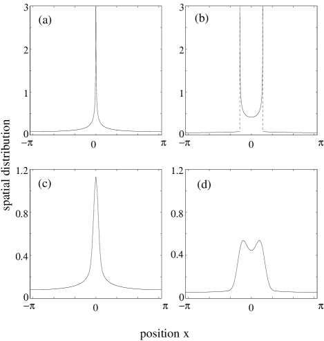
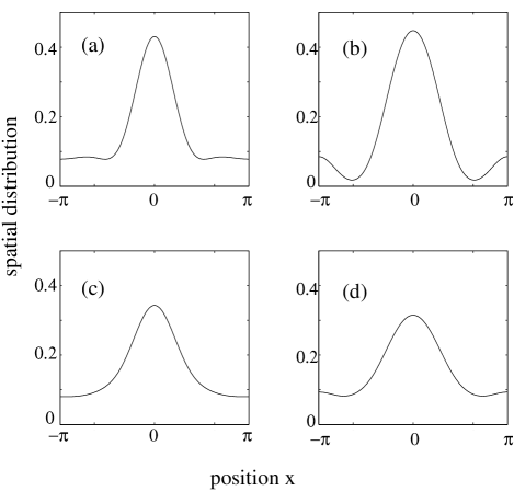
Here the summation is performed over all possible branches of the function $x_{0}(x)$ defined by Eqs. (2) and (3), as described in [32]. Figure 1 displays the spatial distribution of atoms at different times after a single $\delta$-kick. In pictures (a) and (b), the initial temperature of the ensemble is zero. Figure 1 (a) shows the spatial distribution at $\tau=1$ after the pulse. One observes a sharp, narrow peak at $x=0$ above a broad background. The physics behind this feature is similar to the focusing of light rays by an optical lens. Indeed, the velocity of an atom being initially at the position $x$ is $v=-\sin x$. Therefore, atoms with $x<<1$ have a velocity proportional to their initial position, and they all arrive at the focal point $x=0$ at the same focusing time, $\tau_{f}=1$. In this language, the finite width of the focal spot and the broad background are due to the effect of ”spherical aberrations”, that means, due to the deviation of the $\cos x$ potential from the parabolic one. Figures 1 (b) shows the spatial distribution at $\tau=1.84\tau_{f}$, the time of the maximal squeezing (see below). The distribution is characterized by two singularities. The origin of these peaks is due to the coexistence of two counter-propagating groups of atoms, which appear near $x=0$ at $\tau>\tau_{f}$: those that were focused, and those that were not fast enough to reach the focal point $x=0$ at $\tau=\tau_{f}$. This effect is similar to the formation of rainbows in the wave optics [34] and quantum mechanics [35, 36], and it is discussed in detail in [32]. The position of the peaks is

$$x_{c}=\pm\arccos\left(\frac{1}{\tau}\right)\mp\sqrt{\tau^{2}-1}\,\,\,\,(\mbox{mod}\;2\pi).$$ (8)

The two peaks move in the opposite directions, and asymptotically, they have a constant velocity $v=1$, at $\tau\rightarrow\infty.$

A sharp focal spot, and singular-like rainbow peaks are observed only at zero initial temperature. Figures 1 (c) and (d) show the effect of the finite temperature on the dynamics an ensemble of atoms. They present the spatial distribution at focal time $\tau_{f}$ and at $\tau=1.84\tau_{f}$, respectively. Instead of the singularities seen in Figs. 1 (a) and (b), we observe broader spatial structures that are still reminiscent of the focusing phenomenon and the rainbow effect.

In order to characterize the degree of atomic localization (squeezing), we introduce the localization factor $L(\tau)=1-<\cos x(\tau)>$, which can be written as

$$L(\tau) = 1-\int_{-\infty}^{\infty}dv_{0}\int_{-\pi}^{\pi}dx_{0}f(x_{0},v_{0},\tau=0)$$ (9)

$$\times \cos\left(x_{0}-\tau\sin x_{0}+v_{0}\tau\right).$$ (10)

For a thermal initial distribution, Eq.(10) can be rewritten as

$$L(\tau) = 1-\frac{1}{2\pi}\int_{-\infty}^{\infty}dv_{0}f(v_{0})\cos(v_{0}\tau)$$ (11)

$$\times \int_{-\pi}^{\pi}dx_{0}\cos\left(x_{0}-\tau\sin x_{0}\right),$$ (12)

where $f(v_{0})=1/\sqrt{2\pi\sigma_{cl}^{2}}\exp\left[-v_{0}^{2}/(2\sigma_{cl}^{2})\right]$ with $\sigma_{cl}$ defined in Eq. (6). Then,

$$L(\tau)=1-\exp\left[-\frac{\sigma_{cl}^{2}\tau^{2}}{2}\right]J_{1}(\tau),$$ (13)

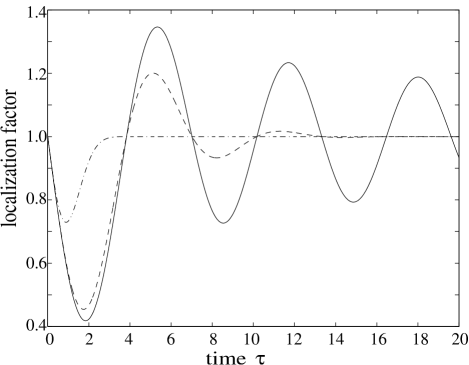
where $J_{1}(\tau)$ is Bessel function of first order. Figure 2 shows the localization factor $L(\tau)$ for different temperatures. At zero temperature (solid line), the localization factor takes the value of $L(\tau_{f})\approx 0.57$ at the focal time $\tau_{f}=1$. Despite the small size of the focal spot, the overall localization is not very marked. This is due to a large fraction of atoms that are out of the focal area. The best localization that can be achieved with a single kick, $L(\tau)\approx 0.42$, occurs after the focal event, at $\tau\approx 1.84$. The spatial distribution at the time of the maximal squeezing for zero temperature can be seen in Fig. 1 (b). For higher initial temperature (dashed and dash-dotted lines in Fig. 2), the best squeezing provided by a single $\delta-$ pulse gets less notable, and it happens at earlier times.

FIG. 2.: Localization factor of a classical ensemble at different temperatures. The solid line displays the localization factor at zero temperature. The dashed and dash-dotted lines correspond to $\sigma_{cl}=0.2$ and $\sigma_{cl}=1$, respectively.

FIG. 3.: Accumulative squeezing. The figure shows the minimal value of the localization factor as a function of the number of kicks. The points (.) correspond to zero initial temperature, the crosses (x) and (+) correspond to $\sigma_{cl}=0.5$ and $\sigma_{cl}=1$, respectively. The graphs are shown in double logarithmic scale.

A Accumulative squeezing

The squeezing can be enhanced by applying multiple short pulses to the atomic system. Recently, the ”accumulative squeezing strategy” for efficient orientation (or alignment) of a kicked rotor was introduced in [32]. In the following, we show that this strategy can be applied to the system of cold atoms driven by a pulsed optical lattice as well. As mentioned above, the spatial distribution of atoms is maximally squeezed at some time $\Delta\tau_{1}$ after the first kick. According to the ”accumulative squeezing strategy”, the second kick is applied exactly at that time, $\tau_{2}=\Delta\tau_{1}$. Immediately after the second kick, the system has the same spatial distribution as before the kick, but $\tau=\tau_{2}$ is no longer a stationary point for the localization factor $L(\tau).$ As a result, $L(\tau)$ will reach a new minimal value at some time point $\tau_{2}+\Delta\tau_{2}$, and this new minimum will be smaller than the previous one. By continuing this way, we apply a sequence of kicks at time instants $\tau_{k+1}=\tau_{k}+\Delta\tau_{k}$, and the squeezing effect accumulates with time. We find the interval $\Delta\tau_{k}$ between the $k$th and $(k+1)$th kicks by minimizing the localization factor

$$L(\tau_{k+1})=1-\frac{1}{2\pi}\int_{-\infty}^{\infty}dv_{0}f(v_{0})\int_{-\pi}^{\pi}dx_{0}\cos x_{k+1},$$ (14)

with respect to $\Delta\tau_{k}$ . Here $x_{k+1}$ is defined by

$$x_{k+1}=x_{k}+\Delta\tau_{k}\left(v_{0}-\sum_{i=1}^{k}\sin x_{i}\right).$$ (15)

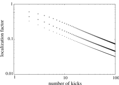
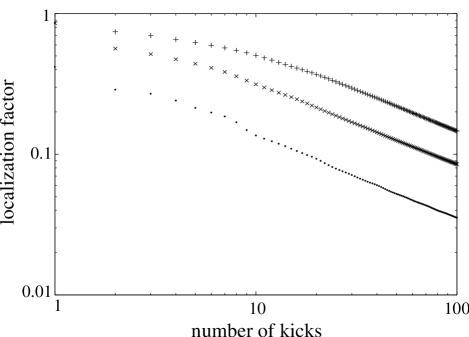
Figure 3 displays $L(\tau_{k})$ for a series of 100 pulses applied at different initial temperature. It can be seen, that after the first few kicks the localization factor demonstrates a negative power dependence as a function of the kick number (a straight line in the double logarithmic scale). The squeezing is reduced for higher initial temperature. However, the slope of all of the curves in Fig. 3 is the same after the first several kicks, in full agreement with the asymptotics $L(\tau_{k})\thicksim 1/\sqrt{k}$ found in [32]. Therefore, the accumulative squeezing scenario may be an effective and regular strategy for atomic localization even at finite temperature. Although finite temperature worsens the squeezing, the temperature effects become less important with increasing the number of kicks. The system gains kinetic energy from each pulse, so eventually the initial thermal energy becomes small compared to the energy supplied by the pulsed optical lattice.

B Optimal squeezing with few short pulses

We have demonstrated that the strategy of accumulative squeezing allows, in principle, an arbitrarily good localization of atoms. However, this does not mean that it is the only one (or the most effective) squeezing strategy. We have studied the best localization that can be achieved with a given number, $N$  of identical $\delta$-kicks, by minimizing the localization factor Eq.(14) in the $N$ -dimensional space of all possible delay times $\Delta\tau_{k}>0$. For clarity, we present here only the results for zero initial atomic temperature. Table I shows the best values of the localization factor found for up to five kicks, and compares them with the results of the accumulative squeezing strategy with the same number of pulses. While the maximal atomic localization for two pulses is almost the same for the accumulative squeezing and for the optimal sequence of two pulses, the optimized results for three and more pulses are much better. The optimized delay times $\Delta\tau_{k}$ between the pulses are shown in Table II. For three and more pulses they differ considerably from the times between kicks according to the accumulative squeezing scheme.

For illustration, we choose the sequence of four optimal pulses to visualize the dynamics behind the squeezing process. First, we note that the second pulse is not applied at the time of the maximal localization. On the contrary, the optimized procedure finds it favorable to wait a bit after the moment of maximal squeezing, until the distribution becomes rather broad.

No of kicks	$L_{acc}$	$L_{op}$
2	0.33	0.31
3	0.26	0.20
4	0.21	0.11
5	0.18	0.07

TABLE I.: Minimal value of the localization factor that can be achieved with a fixed number of kicks using accumulative squeezing scenario ($L_{acc}$) and optimized sequence of pulses ($L_{opt}$).

FIG. 4.: Distribution of particles as a function of their position $x$ and velocity $v$ for a sequence of four optimal pulses. Figs. (a) and (b) are plotted at the time of the first pulse, and before the second pulse, respectively. The distribution after the second pulse, and immediately before the combined third and fourth pulses can be seen in (c) and (d). Finally, the plots (e) and (f) show the distribution immediately after the last pulse and at the time of maximal squeezing. Here, the initial temperature of the ensemble is zero.

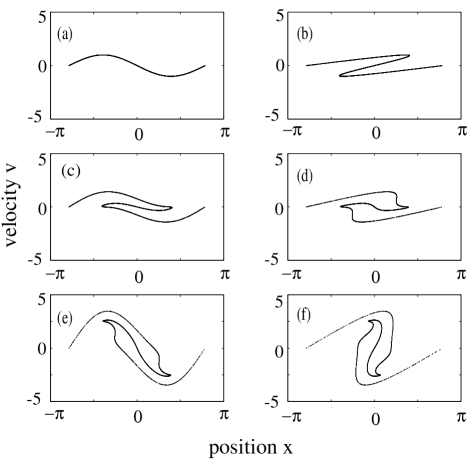
The optimal four-pulse sequence we found requires applying the third and the forth pulses simultaneously, thus producing an effective ”double pulse”. To understand the mechanism of the optimal squeezing with four pulses, we refer to Fig. 4 that shows the velocity of the atoms as a function of their position. The left column displays the velocity immediately after the first (a), the second (c), and combined third and fourth (e) pulses. The right column shows the velocity after the free evolution between the pulses: immediately before the second (b), the third (d) pulse, and at time of the final maximal localization (f). We can see that the first two pulses fold the distribution in a way that most of the atoms are concentrated in the harmonic region around $x=0$ (see Fig. 4 (e)) with a roughly linear dependence of the velocity on the position.

	$\Delta\tau_{1}$	$\Delta\tau_{2}$	$\Delta\tau_{3}$	$\Delta\tau_{4}$
Accumulative squeezing	1.84	0.59	0.42	0.29
Optimal squeezing
2 kicks	1.41
3 kicks	2.73	0
4 kicks	3.02	1.35	0
5 kicks	3.09	1.47	0.12	0.03

TABLE II.: Comparison between the delay times $\Delta\tau_{1}$ - $\Delta\tau_{4}$ for accumulative squeezing and optimal squeezing.

Due to the double strength of the last pulse, it emphasizes the linear character of the velocity distribution. During the free motion of the atoms after the last pulse, the linear-like distribution ”rotates”, so that it becomes concentrated around $x=0$ at the time of the maximal squeezing (see Fig. 4 (f)).

III Quantum squeezing

In order to provide a quantum mechanical description for atoms in a pulsed optical lattice, it is convenient to rescale the variables and the Hamiltonian Eq.(1) in a different way. In the classical limit, there is a single time scale that determines the dynamics of the kicked atoms at zero temperature, namely, the focusing time that depends on the strength of the interaction $V(t)$. However, a quantized space-periodic atomic motion in an optical lattice is characterized by an additional time scale, $\tau_{r}=h/E_{r}$ where $E_{r}=\hbar^{2}(2k_{l})^{2}/2m$ is a kinetic energy of a particle with momentum $2\hbar k_{l}$. This time scale determines the free evolution of an arbitrary atomic state having a spatial period of $\lambda_{l}/2$. Although the energy spectrum of this system is not equidistant, the quantum dynamics of free atoms repeats itself after each period of $4\pi\tau_{r}$. This revival time, which is independent of the interaction strength, provides a criterion for the validity of the classical description of the atom-lattice interaction. If the relevant times are much smaller than $4\pi\tau_{r}$, the system can be considered classically, while for larger times quantum effects become important. We, therefore, introduce the dimensionless time as $\tau=t/\tau_{r}$. Furthermore, we define the dimensionless coordinate as $x^{\prime}=2k_{l}x$, the momentum as $p^{\prime}=p/(2\hbar k_{l})$ and the Hamiltonian as $H^{\prime}=m/(2\hbar k_{l})^{2}H$. The Hamiltonian Eq.(1) can then be rewritten as

$$H(x^{\prime},p^{\prime},\tau)=\frac{p^{\prime}{}^{2}}{2}-V^{\prime}(\tau)\cos x^{\prime}.$$ (16)

The dimensionless field intensity is $V^{\prime}(\tau)=m/(2\hbar k_{l})^{2}V(\tau)$. In what follows, we will drop again  the primes for the clarity of presentation.

If the initial atomic state is a spatially uniform one, or any other state having the same spatial period as the optical lattice, this periodicity property will be preserved in the course of interaction. The wave function of the system can be the expanded in a Fourier series

$$\Psi(x,\tau)=\frac{1}{\sqrt{2\pi}}\sum_{n=-\infty}^{+\infty}c_{n}(\tau)e^{inx}.$$ (17)

In the absence of the field, the time-dependent wave function takes the form

$$\Psi(x,\tau)=\frac{1}{\sqrt{2\pi}}\sum_{n=-\infty}^{+\infty}c_{n}(0)e^{-in^{2}\tau/2+inx}.$$ (18)

FIG. 5.: Probability density at the classical focal time (left column) and at the time of maximal squeezing (right column) for $P=1$. In figures (a) and (b), the initial temperature $T$ is zero, while (c) and (d) correspond to $\sigma_{qm}=0.5$.

Despite the simple form of Eq.(18), the wave function exhibits an extremely rich space-time dynamics. As mentioned before, it shows a periodic time behavior with the period $T_{rev}=4\pi$ (full revival), and a number of fractional revivals at $\tau=p/sT_{rev}$ ($p$ and $s$ are mutually prime numbers) [39]. Hamiltonian (16) is formally equivalent to that one of a 2D driven quantum rotor (if the initial atomic state has a proper space periodicity). An analytical solution valid for a general time-dependent field is not known even for this simplest model. Much effort has been devoted to the excitation by extremely short pulses ($\delta-$kicks) (see, e.g. [40], and references therein). In general, as a result of a single $\delta-$kick applied to the system at $\tau=\tau_{k},$ the coefficients $c_{n}$ transform as

$$c_{n}(\tau_{k}+0)=\sum\limits_{m=-\infty}^{+\infty}i^{n-m}J_{n-m}(P)c_{m}(\tau_{k}-0),$$ (19)

where $P=\int_{-\infty}^{+\infty}V^{\prime}(\tau)d\tau$, and $J_{n}(P)$ is the Bessel function of the $n$th order. The above formulas describe only the evolution of the states with an integer momentum. However, at finite temperature, the initial atomic momentum has a continuous set of values. Taking this into account, we first consider a single, non-integer initial momentum $p_{0}=n_{0}+\nu_{0},$ where $n_{0}$ is the integer part of the dimensionless momentum and $\nu_{0}$ belongs to the interval $[-1/2,1/2)$ (see [37]). Due to the periodicity of the potential, the non-integer part of the initial momentum is preserved during the interaction, so that Eq.(18) may be replaced by

$$\Psi(x,\tau)=\frac{1}{\sqrt{2\pi}}\exp(i\nu_{0}x)\sum_{n=-\infty}^{+\infty}c_{n}(0)e^{-in^{2}\tau/2+inx}.$$ (20)

FIG. 6.: Probability density at the classical focal time (left column) and at the time of maximal squeezing (right column) for $P=10$. In figures (a) and (b), the initial temperature $T$ is zero, while (c) and (d) correspond to $\sigma_{qm}=1$.

At finite temperature $T$, the initial distribution of momentum is

$$\rho(p_{0})=\frac{1}{\sqrt{2\pi}\sigma_{qm}}\exp\left(-\frac{p_{0}^{2}}{2\sigma_{qm}^{2}}\right),$$ (21)

where $\sigma_{qm}=\sqrt{k_{B}Tm}/(2\hbar k_{l})$, with $k_{B}$ being the Boltzmann constant. The averaged spatial probability distribution at time $\tau$ after a kick is then

$$\int_{-\infty}^{\infty}dp_{0}\rho(p_{0})|\Psi(x,\tau)|^{2}$$ (22)

$$= \sum_{n_{0}=-\infty}^{\infty}\int_{-1/2}^{+1/2}d\nu_{0}\rho(n_{0}+\nu_{0})|\Psi(x,\tau)|^{2}.$$ (23)

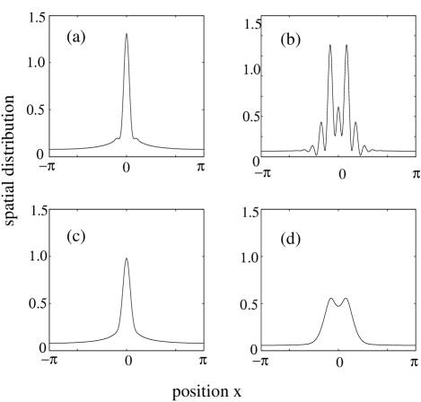
Figures 5 and 6 show the spatial density of atoms after a single $\delta$ -kick, for two different pulse strengths, and different initial temperature. The left columns show the probability density at the classical focal time ($\tau=1/P$), while the right columns display the density at the time of the maximal squeezing. In Fig. 5, the pulse is rather weak ($P=1$), and the quantum mechanical spatial distribution differs considerably from the classical one (compare with Fig. 1). Instead of a sharp focusing spot, a rather broad distribution centered around $x=0$ is observed even at zero temperature (Fig. 5(a)). The finite value of the initial temperature (see Fig. 5 (c) and (d)) broadens the distribution even more. However, for stronger pulses ($P=10$) the quantum-mechanical results (see Fig. 6) resemble the classical ones. At zero temperature, the quantum effects replace the classical singularities by sharp maxima in the probability distribution with the Airy-like shape typical to the rainbow-type scattering in

FIG. 7.: Quantum mechanical localization factor as a function of time. The kick strength is $P=0.5$ and $P=10$ in figures (a) and (b), respectively. The solid lines represent the localization factor at zero initial temperature, the dashed and dash-dotted lines correspond to $\sigma_{qm}=0.2$ and $\sigma_{qm}=1$, respectively.

optics and quantum mechanics [32] (see Fig. 6 (b)). At finite temperature, however, the fine structure is washed out, and the system behaves mainly like a classical ensemble of atoms at finite temperature (compare Figs. 6 (c) and (d) and Fig. 1 (c) and (d)).

We proceed to the calculation of the quantum localization factor $L(\tau)=1-<\cos x>$ for an atomic system subject to a series of short pulses applied at $\tau=\tau_{k}$ ($k=1,2,3,...$). If the initial state contains only a single momentum $p_{0}=n_{0}+\nu_{0},$ the localization factor after the $k$th pulse is

$$L_{p_{0}}(\tau) = 1-Re\sum_{n=-\infty}^{\infty}c_{n}(\tau_{k}+0)c_{n+1}^{\ast}(\tau_{k}+0)$$ (24)

$$\times \exp\left[i\left(n+\nu_{0}+\frac{1}{2}\right)(\tau-\tau_{k})\right].$$ (25)

For a single pulse applied at $\tau=0$, one finds (using Eq. (19) ):

$$L_{p_{0}}(\tau) = 1-\sum_{n=-\infty}^{\infty}J_{n}(P)J_{n+1}(P)\sin\left[\left(n+p_{0}+\frac{1}{2}\right)\tau\right]$$ (26)

$$= 1-\cos\left(p_{0}\tau\right)J_{1}\left(2P\sin\frac{\tau}{2}\right).$$ (27)

If the system is initially in a thermal state, the localization factor has to be averaged over the momentum distribution Eq. (21) ,

$$L(\tau)=\int_{-\infty}^{\infty}dp_{0}\,\rho(p_{0})L_{p_{0}}(\tau).$$ (28)

After the averaging, it and takes the form

$$L(\tau)=1-\exp\left(-\frac{\tau^{2}\sigma_{qm}^{2}}{2}\right)J_{1}\left(2P\sin\frac{\tau}{2}\right).$$ (29)

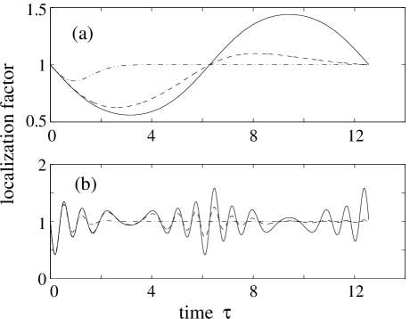
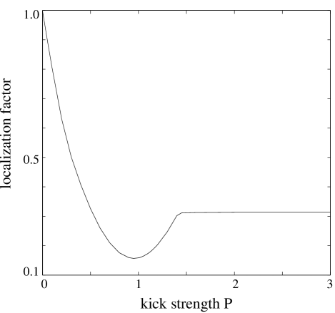
Fig. 7 shows the localization factor as a function of time for various temperatures and kick strengths, $P$. At zero temperature (solid line), the quantum mechanical localization factor shows a revival structure, in contrast to the classical one. The pattern, and, therefore, the state of the maximal localization, repeats itself after each period of $4\pi$. However, due to the continuous character of atomic momentum at finite temperature, the revival structure disappears with increasing the temperature (see dashed and dash-dotted lines in Figs. 7 (a)  and (b)). In Fig. 7 (b), the strength of the kick is $P=10$. Comparing the quantum mechanical localization factor with its classical counterpart (see Fig. 2), we see that they have the same structure for short times, and the same minimal localization factor $L(\tau)\approx 0.42.$ In the short-time limit, $\tau/2\ll 1$, Eq. (29) can be approximated by

$$L(t)\approx 1-\exp\left(-\frac{\sigma_{qm}^{2}\tau^{2}}{2}\right)J_{1}\left(P\tau\right),$$ (30)

which is exactly the expression for the classical localization factor Eq. (13) (we remind about the different time units used in the classical and quantum cases). For $P=10$, maximal squeezing occurs at $\tau=0.18$, and therefore the classical approximation is valid. For smaller values of $P$ (for example $P=0.5$ in Fig. 7 (a)), the quantum mechanical localization factor differs considerably from the classical one. Maximal squeezing occurs only at $\tau\approx 3.1,$ which is well outside the classical region. Moreover, the minimal value of the localization factor is increasing for smaller values of $P$ (for example, $L(\tau)\approx 0.56$ for $P=0.5$). With a single kick, the most profound squeezing can, therefore, be achieved with a relatively strong kick, after which the system behaves more or less classically.

FIG. 8.: Quantum mechanical accumulated squeezing. The figure shows the minimal localization factor (maximal squeezing) as a function of the number of kicks. The kick strength is $P=1$. The points (.) represent the localization factor for zero initial temperature, and the crosses (x) and (+) correspond to $\sigma_{qm}=1$ and $\sigma_{qm}=2$, respectively. The graphs are shown in double logarithmic scale.

FIG. 9.: Minimal localization factor as a function of the kick strength $P$. Here, the optimal sequence of two identical pulses and the resulting minimal localization factor were calculated for different values of $P$. The initial temperature of the atoms is zero.

A Accumulative squeezing vs optimal squeezing in the quantum domain

The accumulative squeezing scenario [32] described above can be applied to the quantized atomic motion as well. Moreover, due to the revival phenomenon, the sequence of pulses can be made ”almost periodic”, $\tau_{k+1}=\tau_{k}+\Delta\tau_{k}+T_{rev}$, where $\Delta\tau_{k}$ is chosen to minimize the atomic localization factor after the $k$th kick. The introduction of the $T_{rev}$-shift between pulses may be useful in practical realizations of the scenario to avoid the overlap between short pulses of a finite duration. Figure 8 demonstrates the validity of the accumulative squeezing scenario in the quantum mechanical regime. For cesium atoms, under conditions of a recent experiment by M. Raizen group [38], the values of $\sigma_{qm}=1$ and $\sigma_{qm}=2$ correspond to the initial temperature of $0.8\mu$K and $3.2\mu$K, respectively. The system demonstrates a reduced squeezing for higher initial temperatures, however, the slope of all of the curves in Fig. 8 becomes the same after the first several pulses, exactly as in the classical case.

In Section II we discussed the optimal sequence of $\delta-$pulses needed to accomplish the maximal squeezing for a given number of kicks. In the classical limit, and at zero temperature condition, the only optimization parameters are the time intervals (measured in the units of the focusing time $\tau_{f})$ between the pulses. However, in the fully quantum mechanical description, the kick strength $P$ is an independent additional parameter. Figure 9 shows the minimal localization factor, that can be gained with two identical $\delta-$ pulses as a function of $P$.

FIG. 10.: Quantum mechanical optimal squeezing with two kicks. The figures show the probability density of the maximally squeezed state for $P=10$ (a) and $P=1$ (b), respectively. Here, the initial temperature of the atoms is zero.

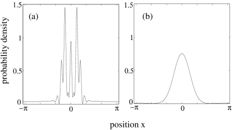
For $P\geq 1.5$, the best possible localization factor is almost independent of $P$. The same value, $L\approx 0.31$, was obtained classically (see Table I). The optimal delay time between the pulses is also in a good agreement with the classical result $P\Delta\tau_{1}=1.4$ (see Table II). However, as can be seen from Fig. 9, a sharp transition occurs at $P\approx 1.5$. For smaller kick strength, the best ”quantum” localization factor depends strongly on $P$, and the ”classical” sequence of pulses is no longer the optimal solution. The localization factor has a minimum at $P\approx 1$, and its value, $L\approx 0.16$, is approximately half of the expected ”classical” value. The time delay between the pulses, $\Delta\tau_{1}\approx 2.69$, is substantially longer compared to the classically calculated interval between the optimal kicks. Figure 10 shows the probability distribution of the maximally squeezed atomic state after the optimal sequence of two pulses. In Fig. 10 (a), the quantum optimization was done for $P=10$. The distribution has a bimodal structure with two typical Airy-like rainbow peaks (compare with the classical rainbow singularities in Fig. 1 (b)). The probability distribution for $P=1$ (see Fig. 10 (b)) is, however, quite different from the classical one.  The width of the central part of the distribution shown in Fig. 10 (b) looks comparable with the width of the distribution in Figs. 10 (a), however the localization factor in considerably smaller due to the suppressed background.

IV Summary

In this paper we presented a theoretical study on the process of a transient squeezing of an ensemble of cold atoms via interaction with a pulsed nonresonant optical lattice. We studied in detail the atomic evolution following a single short pulse, and described a number of semiclassical catastrophes in the time-dependent spatial distribution of atoms, like focusing, and rainbow formation. The problem was treated both classically, and quantum-mechanically, and a clear correspondence between these two descriptions was established. We have demonstrated that using a proper sequence of short laser pulses, it is possible to narrow dramatically the atomic spatial distribution near the minima of the light-induced potential. In particular, we tested the strategy of accumulative squeezing that was suggested recently [32] for the enhanced orientation (alignment) of a quantum rotor (molecule) interacting with short laser pulses. We showed that this approach works effectively for the atomic squeezing, both in zero temperature limit, and at finite temperature. Furthermore, we searched for the optimal squeezing strategies that provide the best possible atomic localization with a given number of short laser pulses. Both classical, and quantum-mechanical optimization was performed. For large enough pulse intensity, the optimal strategy for the best localization follows the classical scenario. For smaller pulse strength, quantum mechanical effects give rise to new localization mechanisms which may be more effective than the ”classical” ones. A detailed study of the optimal squeezing approaches, also at finite temperature, will be published elsewhere.

We are glad to mention that a part of our predictions and conclusions is already supported by a recent experiment [41] by the group of M. Raizen. Using the accumulative squeezing approach, they demonstrated a substantial squeezing of cold cesium atoms kicked by a pulsed optical lattice.

V Acknowledgment

We are pleased to acknowledge fruitful discussions with R. Arvieu, Y. Prior, and M. Raizen. The work of ML was supported in part by the Minerva Foundation.

REFERENCES

- [1] P. S. Jessen and I. H. Deutsch, Adv. Atm. Mol. Opt. Phys. 37, 95 (1996).
- [2] M. BenDahan, E. Peik, J. Reichel, Y. Castin, and C. Salomon, Phys. Rev. Lett. 76, 4508 (1996).
- [3] S. R. Wilkinson, C. F. Bharucha, K. W. Madison, Qian Niu, and M. G. Raizen, Phys. Rev. Lett. 76, 4512 (1996).
- [4] Qian Niu, Xian-Geng Zhao, G. A. Georgakis, and M. G. Raizen, Phys. Rev. Lett. 76, 4504 (1996).
- [5] R. Graham, M. Schlautmann, and P. Zoller, Phys. Rev. A 45, R19 (1992).
- [6] F. L. Moore, J. C. Robinson, C. F. Bharucha, B. Sundaram, and M. G. Raizen, Phys. Rev. Lett. 75, 4598 (1995).
- [7] H. Ammann, R. Gray, I. Shvarchuck, and N. Christensen, Phys. Rev. Lett. 80, 4111 (1998).
- [8] G. Timp, R. E. Behringer, D. M. Tennant, J. E. Cunningham, M. Prentiss, and K. K. Berggren, Phys. Rev. Lett. 69, 1636 (1992).
- [9] J. J. McClelland, R. E. Scholten, E. C. Palm, and R. J. Cellota, Science 262, 877 (1993).
- [10] R. J. Cellota and J. J. McClelland, US Patent 5,360,764 (1994).
- [11] U. Drodofsky, J. Stuhler, B. Brezger, T. Schulze, M. Drewsen, T. Pfau, and J. Mlynek, Microelectronic Engineering 35, 285 (1997).
- [12] R. Gupta, J. J. McClelland, Z. J. Jabbour, and R. J. Cellota, Appl. Phys. Lett. 67, 1378 (1995).
- [13] for a recent review of atom lithography see, e.g. a special issue on nanomanipulation of atoms, Appl. Phys. B 70, issue 5 (2000), edited by D. Meschede and J. Mlynek.
- [14] S. Meneghini, V. I. Savichev, K. A. H. van Leeuwen, and W. P. Schleich, Appl. Phys. B 70, 675 (2000).
- [15] A. Görlitz, M. Weidemüller, T.W. Hänsch, and A. Hemmerich, Phys. Rev. Lett. 78, 2096 (1997)
- [16] G. Raithel, G. Birkl, W. D. Phillips and S. L. Rolston, Phys. Rev. Lett. 78, 2928 (1997).
- [17] P. Rudy, R. Ejnisman, and N. P. Bigelow, Phys. Rev. Lett. 78, 4906 (1997).
- [18] C. Monroe, Nature 388, 719 (Aug 21, 1997).
- [19] G. Birkl, M. Gatzke, I. H. Deutsch, S. L. Rolston, and W. D. Phillips, Phys. Rev. Lett. 75, 2823 (1995).
- [20] M. Weidemüller, A. Hemmerich, A. Görlitz, T. Esslinger, and T. W. Hänsch, Phys. Rev. Lett. 75, 4583 (1995).
- [21] G. Raithel, G. Birkl, A. Kastberg, W. D. Phillips and S. L. Rolston, Phys. Rev. Lett. 78, 630 (1997).
- [22] A. L. Burin, J. L. Birman, A. Bulatov, and H. Rabitz, cond-mat/9708113 (1997).
- [23] A. Bulatov, B. Vugmeister, A. Burin, and H. Rabitz, Phys. Rev. A 58, 1346 (1998).
- [24] A. Bulatov, B. E. Vugmeister, and H. Rabitz, Phys. Rev. A 60, 4875 (1999).
- [25] D. Normand, L. A. Lompre, and C. Cornaggia, J. Phys. B 25, L497 (1992).
- [26] P. Dietrich, D. T. Strickland, M. Laberge, and P. B. Corkum, Phys. Rev. A 47, 2305 (1993).
- [27] B. Friedrich and D. Herschbach, Phys. Rev. Lett. 74, 4623 (1995); J. Phys. Chem. 99, 15686 (1995).
- [28] J. Karczmarek, J. Wright, P. Corkum, and M. Ivanov, Phys. Rev. Lett. 82, 3420 (1999).
- [29] T. Seideman, J. Chem. Phys. 103, 7887 (1995); ibid. 106, 2881 (1997).
- [30] T. Seideman, Phys. Rev. Lett. 83, 4971 (1999).
- [31] L. Cai, J. Marango. and B. Friedrich, Phys. Rev. Lett. 86, 775 (2001).
- [32] I. Sh. Averbukh and R. Arvieu, Phys. Rev. Lett. 87, 163601 (2001).
- [33] I.Sh. Averbukh, patent pending.
- [34] Yu. A. Kravtsov and Yu. I. Orlov, ”Caustics, Catastrophes and Wave Fields” (Springer Series on Wave Phenomena, 15), 2nd edition, (Springer-Verlag, Berlin, 1999).
- [35] K. W. Ford and J. A. Wheeler, Ann. Phys. 7, 259 (1959).
- [36] M. V. Berry, Adv. Phys. 25, 1 (1976).
- [37] C. F. Bharucha, J. C. Robinson, F. L. Moore, Bala Sundaram, Qian Niu, and M. G. Raizen, Phys. Rev. E 60, 3881 (1999).
- [38] W. H. Oskay, D. A. Steck, V. Milner, B. G. Klappauf, and M. G. Raizen, Opt. Comm. 179, 137 (2000) .
- [39] I. Sh. Averbukh and N. F. Perelman, Phys. Lett. A 139, 449 (1989); Sov. Phys. JETP 69, 464 (1989).
- [40] F. Haake, Quantum Signatures of Chaos, Springer Verlag, (Berlin, 1991).
- [41] M. Raizen et al, to be published