Quantum Information Theory
and
Applications to Quantum Cryptography

About this Individual Study Option

In this Individual Study Option the concepts of classical and quantum information theory are presented, with some real-life applications, such as data compression, information transmission over noisy channels and quantum cryptography.

Abstract

In each chapter the following topics are covered:

1. The relation of information theory with physics is studied and by using the notion of Shannon’s entropy, measures of information are introduced. Then their basic properties are proven. Moreover important information relevant features of quantum physics, like the disability of distinguishing or cloning states in general are studied. In order to get a quantum measure of information, an introduction to quantum thermodynamics is given with a special focus on the explanation of the utility of density matrix. After this von Neumann entropy and its related measures are defined. In this context a major discrepancy between classical and quantum information theory is presented: quantum entanglement. The basic properties of von Neumann entropy are proven and some information theoretic interpretation of quantum measurement is given.

2. The amount of accessible information is obtained by the Fano’s inequality in the classical case, and by its quantum analogue and Holevo’s bound in the quantum case. In addition to this classical and quantum data processing is discussed.

3. Furthermore for real-life applications data compression is studied via Shannon’s classical and Schumacher’s quantum noiseless channel coding theorems. Another application is transmission of classical information over noisy channels. For this a summary of classical and quantum error correction is given, and then Shannon’s classical noisy channel and Holevo-Schumacher-Westmoreland quantum noisy channel coding theorems are studied. The present state of transmission of quantum information over quantum channels is summarized.

4. A practical application of the aforementioned is presented: quantum cryptography. In this context the BB84, a quantum key distribution protocol, is demonstrated and its security is discussed. The current experimental status of quantum key distribution is summarized and the possibility of a commercial device realizing quantum cryptography is presented.

Special viewpoints emphasized

The above material is in close connection with the last two chapters of [1, chap.11,12], and error correction is a summary of the results given in chapter 10 of [1]. From this book Figures 1.1, 3.1, 3.2 and S.1, were extracted. However there was much influence on information theory by [2], and some results given therein like for example equation (3.1.1) were extended to (3.2). Of equal impact was [3] concerning error correction, and [3, 4] concerning quantum cryptography. Note that Figure was 4.2 extracted from [4]. Of course some notions which were vital to this Individual Study Option were taken from almost all the chapters of [1].

However there where some topics not well explained or sometimes not enough emphasized. The most important tool of quantum information theory, the density matrix, is misleadingly given in [1, p.98]: ”the density matrix […] is mathematically equivalent to the state vector approach, but it provides a much more convenient language for thinking about commonly encountered scenarios in quantum mechanics”. The density matrix is not equivalent to the state vector approach and is much more than just a convenient language. The former is a tool for quantum thermodynamics, a field where is impossible to use the latter. Rephrasing it, quantum thermodynamics is the only possible language. Willing to augment understanding of this meaningful tool, subsection 1.2.2 is devoted to it, and is close to the viewpoint of [5, p.295-307], which is a classical textbook for quantum mechanics.

In this Individual Study Option some topics are presented in a different perspective. There is an attempt to emphasize information theoretic discrepancies between classical and quantum information theory, the greatest of which is perhaps quantum entanglement. A very special demonstration of this difference is given in subsection 1.2.4. It should be noted that some particular information theoretic meaning of measurement in physics is presented in subsection 1.2.6.

Concerning the different views presented in this text, nothing could be more beneficial than the 64 exercises of the last two chapters of [1, chap.11,12]. As an example a delicate presentation of measures of information is given in page 1.1, due to exercise 11.2 [1, p.501], or subsection 1.2.4 on quantum entanglement was inspired by exercise 11.14 [1, p.514]. In some occasions special properties where proved in order to solve the exercises. Such a property is the preservation of quantum entropy by unitary operations (property 2 of von Neumann entropy, in page 2), which was needed to solve for example exercise 11.19,20 [1, p.517,518]. For these last two exercises some special lemmas were proven in appendices A.1 and A.2. It is important to notice that from the above mentioned exercises of [1, chap.11,12] only half of them are presented here.

Notation

Finally about the mathematical notation involved, the symbol $\triangleq$ should be interpreted as ”defined by”, and the symbol $\equiv$ as ”to be identified with”.

Chapter 1 Physics and information theory

Since its invention, computer science [6] was considered as a branch of mathematics, in contrast to information theory [7, 8] which was viewed by its physical realization; quoting Rolf Landauer [9] ”information is physical”. The last decades changed the landscape and both computers and information are mostly approached by their physical implementations [10, 11, 12, 13]. This view is not only more natural, but in the case of quantum laws it gives very exciting results and sometimes an intriguing view of what information is or can be. Such an understanding could never be inspired just from mathematics. Moreover there is a possibility that the inverse relation exists between physics and information [14, 15] or quoting Steane [3] one could find a new methods of studying physics by ”the ways that nature allows, and prevents, information to be expressed and manipulated, rather than [the ways it allows] particles to move”. Such a program is still in its infancy, however one relevant application is presented in subsection 1.2.6. In this chapter the well established information theory based on classical physics is presented in section 1.1, and the corresponding up to date known results for quantum physics are going to be analyzed in section 1.2.

1.1 Classical physics and information theory

In classical physics all entities have certain properties which can be known up to a desired accuracy. This fact gives a simple pattern to store and transmit information, by assigning information content to each of the property a physical object can have. For example storage can be realized by writing on a paper, where information lays upon each letter, or on a magnetic disk, where information, in binary digits (bits), is represented each of the two spin states a magnetic dipole can have. In what concerns transmission, speech is one example, where each sound corresponds to an information, or a second example is an electronic signal on a wire, where each state of the electricity is related to some piece of information. Unfortunately in every day life such simple patterns are non-economical and unreliable. This is because communication is realized by physical entities which are imperfect, and hence they can be influenced by environmental noise, resulting information distortion.

Concerning the economical transmission of information, one can see that the naive pattern of information assignment presented in the last paragraph is not always an optimal choice. This is because a message, in English language for example, contains symbols with different occurrence frequencies. Looking for example this text one can note immediately that the occurrence probability of letter a, $p_{\mathtt{a}},$ is much greater than that of exclamation $p_{\text{{!}}}.$ According to the naive assignment, English language symbols are encoded to codewords of identical length $l$, and the average space needed to store $\mathtt{a}$ is $lp_{\mathtt{a}}$ and of the exclamation $lp_{\text{{!}}},$ and since $p_{\mathtt{a}}>p_{\text{{!}}}$, a lot of space is wasted for the letter $\mathtt{a}$. In order to present how a encoding scheme can be economical consider a four letter alphabet A, B, C, D, with occurrence probabilities $p_{\mathtt{A}}=\frac{3}{4},$ $p_{\mathtt{B}}=\frac{1}{8},$ $p_{\mathtt{C}}=p_{\mathtt{D}}=\frac{1}{16},$ the subsequent assignment of bits: $\mathtt{A}\rightarrow 1,$ $\mathtt{B}\rightarrow 01,$ $\mathtt{C}\rightarrow 010,$ and $\mathtt{D}\rightarrow 011$. A message of $n$ symbols, using this encoding, has on average $n\left(p_{\mathtt{A}}+2p_{\mathtt{B}}+3p_{\mathtt{C}}+3p_{\mathtt{D}}\right)=n\left(\frac{3}{4}+2\frac{1}{8}+3\frac{1}{16}+3\frac{1}{16}\right)=n\left(\frac{11}{8}\right)$ bits instead of $2n$ which would needed if somebody just mapped to each letter a two bit codeword.

The topics discussed in the last two paragraphs give rise to the most important information theoretic question: which are the minimal resources needed to reliably communicate? An answer to this question can be given by abstractly quantifying information in relevance to the physical resources needed to carry it. Motivated by the previously demonstrated four letter alphabet example, probabilities are going to be used for such an abstraction. One now defines a function $H,$ quantifying a piece of information $I,$ exhibiting the following reasonable properties:

1. $H\left(I\right)$ is a function only of the probability of occurrence $p$ of information $I,$ thus $H\left(I\right)\equiv H\left(p\right).$

2. $H$ is a smooth function.

3. The resources needed for two independent informations with individual probabilities $p,q>0\$are the sum of the resources needed for one alone, or in mathematical language $H\left(pq\right)=H\left(p\right)+H\left(q\right).$

The second and third property imply that $H$ is a logarithmic function, and by setting $q=1$ in the third it is immediate to see that $H\left(1\right)=0.$ Hence $H\left(p\right)=k\log p,$ where $k$ and $a$ are constants to be determined (refer to comments after equations (1.2) and (1.5)). This means that the average of resources needed when one of the mutually exclusive set of information with probabilities $p_{1},\ldots,p_{n}$ occurs is

$$H\left(p_{1},\ldots,p_{n}\right)=k\sum_{i}p_{i}\log_{a}p_{i}.$$ (1.1)

It should be noted that probability is not the only way of quantifying information [14, 15, 16, 17, 18, 19].

1.1.1 Shannon entropy and relevant measures of classical information theory

The function $Q$ found in (1.1) is known in physics as entropy, and measures the order of a specific statistical system. Of course one interesting physical system is an $n$-bit computer memory, and if all the possible cases of data entry are described by a random variable $X$ with probabilities $p_{1},\ldots,p_{2^{n}},$ then the computer’s memory should have an entropy given by

$$H\left(X\right)\equiv H\left(p_{1},\ldots,p_{2^{n}}\right)\triangleq-\underset{x}{\sum}p_{x}\log p_{x}.$$ (1.2)

Here a modified version of (1.1) is used, with $\log\equiv\log_{2}$ and $k\triangleq 1,$ an assignment to be verified after equation (1.5). Equation (1.2) is known in information theory as the Shannon’s entropy [7]. There are two complementary ways of understanding Shannon’s entropy. It can be considered as a measure of uncertainty before learning the value of a physical information or the information gain after learning it.

The Shannon entropy gives rise to other important measures of information. One such is the relative entropy, which is defined by

$$H\left(p_{x}||q_{x}\right)\triangleq\underset{x}{\sum}p_{x}\log\frac{p_{x}}{q_{x}}=-H\left(X\right)-\underset{x}{\sum}p_{x}\log q_{x},$$ (1.3)

and is a measure of distance between two probability distributions. This is because it can be proven that

$$H\left(p_{x}||q_{x}\right) > 0,$$ (1.4)

$$H\left(p_{x}||q_{x}\right) = 0\Leftrightarrow\forall x:p_{x}=q_{x}.$$

Of course it is not a metric because as one can check $H\left(p_{x}||q_{x}\right)=H\left(q_{x}||p_{x}\right)$ is not always true. The relative entropy is often useful, not in itself, but because it helps finding important results. One such is derived using the last equality in (1.3) and (1.4), then in a memory with $n$-bits

$$H\left(X\right) < \log 2^{n}=n,$$ (1.5)

$$H(X) = \log 2^{n}=n\Leftrightarrow\forall i:p_{i}=\frac{1}{2^{n}},$$

which justifies the selection of $k=1$ in (1.2), because in the optimal case and in absence of noise, the maximum physical resources needed to transmit or to store an $n$-bit word should not exceed $n$. One can also see from (1.2) that

$$H\left(X\right) > 0,$$ (1.6)

$$H\left(X\right) = 0\Leftrightarrow\text{system }X\text{ is in a definite state (}p=1\text{).}$$

Other important results are deduced relative entropy, and concern useful entropic quantities such as the joint entropy, the entropy of $X$ conditional on knowing $Y,$ and the common or mutual information of $X$ and $Y.$ Those entropies are correspondingly defined by the subsequent intuitive relations

$$H\left(X,Y\right) \triangleq -\sum_{xy}p_{xy}\log p_{xy},$$ (1.7)

$$H\left(X|Y\right) \triangleq H\left(X,Y\right)-H\left(Y\right),$$ (1.8)

$$H\left(X:Y\right) \triangleq H\left(X\right)+H\left(Y\right)-H\left(X,Y\right)=H\left(X\right)-H\left(X|Y\right),$$ (1.9)

and can be represented in the ’entropy Venn diagram’ as shown in Figure 1.1.

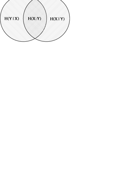
Figure 1.1: Relationships between different entropies.

1.1.2 Basic properties of Shannon entropy

It is worth mentioning here the basic properties of Shannon entropy:

1. $H\left(X,Y\right)=H\left(Y,X\right),$ $H\left(X:Y\right)=H\left(Y:X\right).$

2. $H\left(Y|X\right)\geq 0$ and thus by the second equality of (1.9) $H\left(X:Y\right)\leq H\left(Y\right),$ with equality if and only if $Y$ is a function of $X,$ $Y=f\left(X\right).$

3. $H\left(X\right)\leq H\left(X,Y\right),$ with equality if and only if $Y$ is a function of $X.$

4. Subadditivity: $H\left(X,Y\right)\leq H\left(X\right)+H\left(Y\right)$ with equality if and only if $\ X$ and $\ Y$ are independent random variables.

5. $H\left(Y|X\right)\leq H\left(Y\right)$ and thus by the second equality of (1.9) $H\left(X:Y\right)\geq 0,$ with equality in each if and only if $X$ and $Y$ are independent variables.

6. Strong subadditivity: $H\left(X,Y,Z\right)+H\left(X\right)\leq H\left(X,Y\right)+H\left(Y,Z\right),$ with equality if and only if $Z\rightarrow Y\rightarrow X$ forms a Markov chain.

7. Conditioning reduces entropy: $H\left(X|Y,Z\right)\leq H\left(X|Y\right).$

8. Chaining rule for conditional entropies: Let $X_{1},\ldots,X_{n}$ and $Y$ be any set of random variables, then $H\left(X_{1},\ldots,X_{n}|Y\right)=\sum_{i=1}^{n}H\left(X_{i}|Y,X_{1},\ldots,X_{i-1}\right).$

9. Concavity of the entropy: Suppose there are probabilities $q_{i}\geq 0,$ $p_{i}>0$ and then $H\left(\sum_{i}p_{i}q_{j}\right)\geq\sum_{i}p_{i}H\left(q_{j}\right),$ with equality if and only if $q_{j}$s are identical.

The various relationships between entropies may mostly be derived from the ’entropy Venn diagram’ shown in Figure 1.1. Such figures are not completely reliable as a guide to properties of entropy, but they provide a useful mnemonic for remembering the various definitions and properties of entropy. The proofs of the above mentioned properties follow.

Proof

1. Obvious from the definition of joint entropy (1.7) and mutual entropy (1.9).

2. Based on the definition of conditional entropy (1.8)

   $$H\left(Y|X\right) \triangleq H\left(X,Y\right)-H\left(Y\right)=-\sum_{xy}p\left(x,y\right)\log p\left(x,y\right)+\sum_{x}p\left(y\right)\log p\left(y\right)$$

   $$= -\sum_{xy}p\left(x,y\right)\log p\left(x,y\right)+\sum_{xy}p\left(x,y\right)\log p\left(y\right)=-\sum_{xy}p\left(x,y\right)\log\frac{p\left(x,y\right)}{p\left(y\right)}$$

   $$= -H\left(p\left(x,y\right)||p\left(y\right)\right),$$

   and using (1.4), where equality holds if and only if $p\left(X,Y\right)=p\left(Y\right),$ that is $Y=f\left(X\right).$

3. It is immediately proven by the second one and using the definition of conditional entropy (1.8).

4. Following the subsequent steps of calculation

   $$H\left(p\left(x,y\right)||p\left(x\right)p\left(y\right)\right) \triangleq -H\left(p\left(x,y\right)\right)-\sum_{xy}p\left(x,y\right)\log p\left(x\right)p\left(y\right)$$

   $$= -H\left(p\left(x,y\right)\right)-\sum_{xy}p\left(x,y\right)\log p\left(x\right)-\sum_{xy}p\left(x,y\right)\log p\left(y\right)$$

   $$= -H\left(p\left(x,y\right)\right)+H\left(p\left(x\right)\right)+H\left(p\left(y\right)\right),$$

   where the second equality of (1.3) was used. The result follows directly from equation (1.4).

5. It is easily derived from subadditivity (property 4) and the definition of conditional entropy (1.8).

6. First note that by the definition of the joint entropy (1.7) and some algebra $H\left(X,Y,Z\right)+H\left(Y\right)-H\left(X,Y\right)-H\left(Y,Z\right)=\sum_{x,y,z}p\left(x,y,z\right)\log\frac{p\left(x,y\right)p\left(y,z\right)}{p\left(x,y,z\right)p\left(y\right)}.$ Then using the fact that $\log x\leq\frac{x-1}{\ln 2}$ for all positive $x$ and equality achieved if and only if $x=1,$ the following can be concluded

   $$\sum_{xyz}p\left(x,y,z\right)\log\frac{p\left(x,y\right)p\left(y,z\right)}{p\left(x,y,z\right)p\left(y\right)} \leq \sum_{xyz}\frac{p\left(x,y,z\right)}{\ln 2}\left(\frac{p\left(x,y\right)p\left(y,z\right)}{p\left(x,y,z\right)p\left(y\right)}-1\right)$$

   $$= \frac{1}{\ln 2}\left(\sum_{y}\frac{p\left(y\right)p\left(y\right)}{p\left(y\right)}\right)-\frac{1}{\ln 2}=0,$$

   with equality if and only if $\frac{p\left(x,y\right)p\left(y,z\right)}{p\left(x,y,z\right)p\left(y\right)}=1\Leftrightarrow p\left(z|y\right)=p\left(z|x,y\right)\Leftrightarrow X\rightarrow Y\rightarrow Z$ is a Markov chain, q.e.d.

7. From strong subadditivity (property 6) it straightforward that $H\left(X,Y,Z\right)-H\left(Y,Z\right)\leq H\left(X,Y\right)-H\left(Y\right)$ and from the definition of conditional entropy (1.26c) the result is obvious.

8. First the result is proven for $n=2$ using the definition of conditional entropy (1.26c)

   $$H\left(X_{1},X_{2}|Y\right) = H\left(X_{1},X_{2},Y\right)-H\left(Y\right)=H\left(X_{1},X_{2},Y\right)-H\left(X_{1},Y\right)+H\left(X_{1},Y\right)-H\left(Y\right)$$

   $$= H\left(X_{2}|Y,X_{1}\right)+H\left(X_{1}|Y\right).$$

   Now induction is going to be used to prove it for every $n$. Assume that the result holds for $n,$ then using the one for $n=2,$ $H\left(X_{1},\ldots,X_{n+1}|Y\right)=H\left(X_{2},\ldots,X_{n+1}|Y,X_{1}\right)+H\left(X_{1}|Y\right),$ and applying the inductive hypothesis to the first term on the right hand side gives

   $$H\left(X_{1},\ldots,X_{n+1}|Y\right)=\sum_{i=2}^{n+1}H\left(X_{i},\ldots,X_{n+1}|Y,X_{i-1}\right)+H\left(X_{1}|Y\right)=\sum_{i=1}^{n+1}H\left(X_{i},\ldots,X_{n+1}|Y,X_{i-1}\right),$$

   q.e.d.

9. The concavity of Shannon entropy, will be deduced by the concavity of von Neumann’s entropy in 1.38. However here is going to be demonstrated that binary entropy ($H_{\text{bin}}\left(p\right)\triangleq H\left(p,1-p\right)$) is strictly concave,

   $$H_{\text{bin}}\left(px_{1}+\left(1-p\right)x_{2}\right)\geq pH_{\text{bin}}\left(x_{1}\right)+\left(1-p\right)H_{\text{bin}}\left(x_{2}\right),$$

   where $0\leq p,x_{1},x_{2}\leq 1$ and equality holds for the trivial cases $x_{1}=x_{2},$ or $p=0,$ or $p=1.$ This is easily proved by using the fact that the logarithmic function is increasing and $-p\left(1-x\right)\geq-\left(1-px\right),$ hence

   $$H_{\text{bin}}\left(px_{1}+\left(1-p\right)x_{2}\right) \triangleq -\left(px_{1}+\left(1-p\right)x_{2}\right)\log\left(px_{1}+\left(1-p\right)x_{2}\right)$$

   $$-\left[1-\left(px_{1}+\left(1-p\right)x_{2}\right)\right]\log\left[1-\left(px_{1}+\left(1-p\right)x_{2}\right)\right]$$

   $$\geq -px_{1}\log x_{1}-\left(1-p\right)x_{2}\log x_{2}-p\left(1-x_{1}\right)\log\left(1-px_{1}\right)$$

   $$-\left(1-p\right)\left(1-x_{2}\right)\log\left[1-\left(1-p\right)x_{2}\right]$$

   $$= pH_{\text{bin}}\left(x_{1}\right)+\left(1-p\right)H_{\text{bin}}\left(x_{2}\right).$$

   The strictness of concave property is seen by noting that only in the trivial cases inequalities such as $\log px_{1}\leq\log\left(px_{1}+\left(1-p\right)x_{2}\right)$ could be equalities. Finally concerning the binary entropy it is obvious that because $\frac{d}{dp}H_{\text{bin}}\left(p\right)=-\log p-1+\log\left(1-p\right)+1=0\Leftrightarrow p=\frac{1}{2},$ and for $p\neq 0,1,$ $\frac{d^{2}}{dp^{2}}H_{\text{bin}}\left(p\right)=-\frac{1}{p}-\frac{1}{1-p}<0,$ the maximum is reached at $p=\frac{1}{2}.$

Some additional notes on the properties of Shannon entropy

Concluding the properties of Shannon entropy, it should be noted that the mutual information is not always subadditive or superadditive. One counterexample for the first is the case where $X$ and $Y$ are independent identically distributed random variables taking the values 0 or 1 with half probability. Let $Z=X\oplus Y,$ where $\oplus$ the modulo 2 addition, then $H\left(X,Y:Z\right)=1$ and further calculating $H\left(X:Z\right)+H\left(Y:Z\right)=0,$ that is

$$H\left(X,Y:Z\right)\nleq H\left(X:Z\right)+H\left(Y:Z\right).$$

The counterexample concerning the second case is the case of a random variable $X_{1}$ taking values 0 or 1 with half probabilities and $X_{2}\triangleq Y_{1}\triangleq Y_{2}\triangleq X_{1}.$ Then $H\left(X_{1}:Y_{1}\right)+H\left(X_{2}:Y_{2}\right)=2$ and in addition to this $H\left(X_{1},X_{2}:Y_{1},Y_{2}\right)=1,$ which means that

$$H\left(X_{1}:Y_{1}\right)+H\left(X_{2}:Y_{2}\right)\nleq H\left(X_{1},X_{2}:Y_{1},Y_{2}\right).$$

1.2 Quantum physics and information theory

Quantum theory is another very important area of physics, which is used to describe the elementary particles that make up our world. The laws and the intuition of quantum theory are totally different from the classical case. To be more specific quantum theory is considered as counter intuitive, or quoting Richard Feynman, ”nobody really understands quantum mechanics”. However quantum physics offers new phenomena and properties which can change peoples view for information. These properties are going to be investigated in this section.

1.2.1 Basic features of quantum mechanics relevant to information theory

Mathematically quantum entities are represented by Hilbert space vectors $\left|\psi\right\rangle,$ usually normalized $\left\langle\psi|\psi\right\rangle=1.$ Quantum systems evolve unitarily, that is, if a system is initially in a state $\left|\psi_{1}\right\rangle,$ it becomes later another state $\left|\psi_{2}\right\rangle$ after a unitary operation

$$U\left|\psi_{1}\right\rangle=\left|\psi_{2}\right\rangle.$$ (1.10)

Unitary operations are reversible, since $UU^{\dagger}=1$ and previous states can be reconstructed by $\left|\psi_{1}\right\rangle=U^{\dagger}\left|\psi_{2}\right\rangle.$ What is important about such operations is that because $\left\langle\psi_{2}|\psi_{2}\right\rangle=\left\langle\psi_{1}\right|U^{\dagger}U\left|\psi_{1}\right\rangle=\left\langle\psi_{1}\right|I\left|\psi_{1}\right\rangle=1,$ normalization, which soon will be interpreted as probability, is conserved. The measurement of the properties of these objects is described by a collection of operators $\left\{M_{m}\right\}.$ The quantum object will found to be in the $m$-th state with probability

$$p\left(m\right)=\left\langle\psi\right|M_{m}^{\dagger}M_{m}\left|\psi\right\rangle,$$ (1.11)

and after this measurement it is going to be in definite state, possibly different from the starting one

$$\frac{M_{m}}{\sqrt{\left\langle\psi\right|M_{m}^{\dagger}M_{m}\left|\psi\right\rangle}}\left|\psi\right\rangle.$$ (1.12)

Of course $m$ should be viewed as the measurement outcome, hence information extracted from a physical system. This way information content can be assigned to each state of a quantum object. As a practical example, in each energy state of an atom one can map four numbers or in each polarization state of a photon one can map two numbers say 0 and 1. The last case is similar to bits of classical information theory, but because a photon is a quantum entity they are named qubits (quantum bits). It should be stressed here that the measurement operators should satisfy the completeness relation $\sum_{m}M_{m}^{\dagger}M_{m}=I$ which results $\sum_{m}p\left(m\right)=\sum_{m}\left\langle\psi\right|M_{m}^{\dagger}M_{m}\left|\psi\right\rangle=1$ as instructed by probability theory. However this implies that $\left\langle\psi\right|M_{m}^{\dagger}M_{m}\left|\psi\right\rangle\neq 1$ and looking at equation (1.12) one understands that measurement is an irreversible operation.

What is very interesting about quantum entities is that they can either be in a definite state or in a superposition of states! Mathematically this is written

$$\left|\psi\right\rangle=\underset{s}{\sum}c_{s}\left|s\right\rangle.$$

Using the language of quantum theory $\left|\psi\right\rangle$ is in state $\left|s\right\rangle$ with probability $c_{s}^{\ast}c_{s},$ and because of normalization the total probability of measuring $\left|\psi\right\rangle$ is

$$\left\langle\psi|\psi\right\rangle=\sum_{s}c_{s}^{\ast}c_{s}=1.$$ (1.13)

States $\left|s\right\rangle$ are usually orthonormal to each other, hence

$$\left\langle\psi|s\right\rangle=c_{s}.$$ (1.14)

Although being simultaneously in many states sounds weird, quantum information can be very powerful in computing. Suppose some quantum computer takes as input quantum objects, which are in a superposition of multiple states, then the output is going to be quantum objects which of course are going to be in multiple states too. This way one can have many calculations done only by one computational step! However careful extraction of results is needed [13, 20, 21, 22, 23], because quantum measurement has as outcome only one answer from the superposition of multiple states, as equation (1.12) instructs, and further information is lost. Then one can have incredible results, like for example calculate discrete logarithms and factorize numbers in polynomial time [20, 21], or search an unsorted database of $N$ objects with only $\sqrt{N}$ iterations [22, 23]!

In contrast to classical information which under perfect conditions can be known up to a desired accuracy, quantum information is sometimes ambiguous. This is because one cannot distinguish non-orthogonal states reliably. Assuming for a while that such a distinction is possible for two non-orthogonal states $\left|\psi_{1}\right\rangle$ and $\left|\psi_{2}\right\rangle$ and a collection of measurement operators $\left\{M_{m}\right\}.$ Then according to this assumption some of the measuring operators give reliable information whether the measured quantity is $\left|\psi_{1}\right\rangle$ or $\left|\psi_{2}\right\rangle,$ and collecting them together the following two distinguishing POVM elements can be defined

$$E_{i}\triangleq\underset{M_{m}\text{ measuring }i}{\sum}M_{m}^{\dagger}M_{m},\text{ }i=1,2.$$

The assumption that these states can be reliably distinguished, is expressed mathematically

$$\left\langle\psi_{i}\right|E_{i}\left|\psi_{i}\right\rangle=1,\text{ }i=1,2.$$ (1.15)

Since $\sum_{i=1,2}E_{i}=I$ it follows that $\sum_{i=1,2}\left\langle\psi_{1}\right|E_{i}\left|\psi_{1}\right\rangle=1.$ Because $E_{1}$ operator reliable measures the first state, then $\left\langle\psi_{1}\right|E_{1}\left|\psi_{1}\right\rangle=1,$ hence the other term must be

$$\left\langle\psi_{1}\right|E_{2}\left|\psi_{1}\right\rangle=0.$$ (1.16)

Suppose $\left|\psi_{2}\right\rangle$ is decomposed in $\left|\psi_{1}\right\rangle$ and and orthogonal state to $\left|\psi_{1}\right\rangle,$ say $\left|\psi_{\perp}\right\rangle;$ then $\left|\psi_{2}\right\rangle=\alpha\left|\psi_{1}\right\rangle+\beta\left|\psi_{\perp}\right\rangle.$ Of course $\left|\alpha\right|^{2}+\left|\beta\right|^{2}=1$ and $\left|\beta\right|<1$ because $\left|\psi_{1}\right\rangle$ and $\left|\psi_{2}\right\rangle$ are not orthogonal. Using the last decomposition and (1.16) $\left\langle\psi_{2}\right|E_{2}\left|\psi_{2}\right\rangle=\left|\beta\right|^{2}\left\langle\psi_{\perp}\right|E_{2}\left|\psi_{\perp}\right\rangle\leq\left|\beta\right|^{2}<1$ which is in contradiction with (1.15).

In what concerns the results of the last paragraph it should be additionally mentioned that information gain implies disturbance. Let $\left|\psi\right\rangle$ and $\left|\phi\right\rangle$ be non-orthogonal states, without loss of generality assume that a unitary process is used to obtain information with the aid of an ancilla system $\left|u\right\rangle$. Assuming that such a process does not disturb the system, then in both cases, one obtains

$$\left|\psi\right\rangle\otimes\left|u\right\rangle \rightarrow \left|\psi\right\rangle\otimes\left|v\right\rangle,$$

$$\left|\phi\right\rangle\otimes\left|u\right\rangle \rightarrow \left|\phi\right\rangle\otimes\left|v^{\prime}\right\rangle.$$

Then one would like $\left|v\right\rangle$ and $\left|v^{\prime}\right\rangle$ to be different, in order to acquire information about the states. However since the inner products are preserved under unitary transformations, $\left\langle v|v^{\prime}\right\rangle\left\langle\psi|\phi\right\rangle=\left\langle u|u\right\rangle\left\langle\psi|\phi\right\rangle\Rightarrow\left\langle v|v^{\prime}\right\rangle=\left\langle u|u\right\rangle=1,$ and hence are identical. Thus distinguishing between $\left|\psi\right\rangle$ and $\left|\phi\right\rangle$ must inevitably disturb at least one of these states.

However at least theoretically there is always a way of distinguishing orthonormal states. Suppose $\left|i\right\rangle$ are orthonormal, then it is straightforward to define the set of operators $M_{i}\triangleq\left|i\right\rangle\left\langle i\right|$ plus the operator $M_{0}\triangleq\sqrt{I-\sum_{i\neq 0}\left|i\right\rangle\left\langle i\right|},$ which satisfy the completeness relation. Now if the state $\left|i\right\rangle$ is prepared then $p\left(i\right)=\left\langle i\right|M_{i}^{\dagger}M_{i}\left|i\right\rangle=1,$ thus they are reliably distinguished.

Another very surprising result is the prohibition of copying arbitrary quantum states. This is known as no-cloning theorem [24, 25] and it can be very easily proven. Suppose it is possible to have a quantum photocopying machine, which will have as input a quantum white paper $\left|w\right\rangle$ and a state to be copied. The quantum photocopying machine should be realized by a unitary transformation $U$ and if somebody tries to photocopy two states $\left|\psi\right\rangle$ and $\left|\phi\right\rangle,$ it should very naturally work as follows

$$U\left\{\left|w\right\rangle\otimes\left|\psi\right\rangle\right\} = \left|\psi\right\rangle\otimes\left|\psi\right\rangle,$$

$$U\left\{\left|w\right\rangle\otimes\left|\phi\right\rangle\right\} = \left|\phi\right\rangle\otimes\left|\phi\right\rangle.$$

Now taking the inner product of these relations $\left\langle\psi|\phi\right\rangle=\left\langle\psi|\phi\right\rangle^{2},$ thus $\left\langle\psi|\phi\right\rangle=0$ or $\left\langle\psi|\phi\right\rangle=1,$ hence $\left|\psi\right\rangle=\left|\phi\right\rangle$ or $\left|\psi\right\rangle$ and $\left|\phi\right\rangle$ are orthogonal. This means that cloning is allowed only for orthogonal states! Thus at least somebody can construct a device, by quantum circuits, to copy orthogonal states. For example if $\left|\psi\right\rangle$ and $\left|\phi\right\rangle$ are orthogonal then there exists a unitary transformation $U$ such that $U\left|\psi\right\rangle=\left|0\right\rangle$ and $U\left|\phi\right\rangle=\left|1\right\rangle.$ Then by applying the FANOUT quantum gate, which maps the input to $\left|00\right\rangle$ if the input qubit was $\left|0\right\rangle$ and to $\left|11\right\rangle$ if the it was $\left|1\right\rangle,$ and further applying $U^{\dagger}\otimes U^{\dagger}$ to the tensor product of outcoming qubits, then either the state $\left|\psi\right\rangle$ is will be copied and finally get $\left|\psi\psi\right\rangle,$ or $\left|\phi\right\rangle$ and get $\left|\phi\phi\right\rangle.$

The basic information relevant features of quantum mechanics, analyzed in this subsection, are summarized in Figure 1.2.

Basic features of quantum mechanics 1. Reversibility of quantum operations 2. Irreversibility of measurement 3. Probabilistic outcomes 4. Superposition of states 5. Distinguishability of orthogonal states by operators 6. Non-distinguishability of non-orthogonal states 7. Information gain implies disturbance 8. Non-cloning of non-orthogonal states

Figure 1.2: A summary of basic information relative features, of quantum mechanics.

1.2.2 The language of quantum information theory: quantum thermodynamics

As in the case of classical information theory thermodynamics should be studied for abstracting quantum information. As it was already stated in the last paragraphs, quantum mechanics have some sort of built-in probabilities. However this is not enough. The probabilistic features of quantum states are different from that of classical thermodynamics. The difference is demonstrated by taking two totally independent facts $A$ and $B.$ Then the probability of both of them occurring would be $P_{AB}^{\text{classical}}=P\left(A\right)+P\left(B\right).$ In contrast, in quantum mechanics the wave functions should be added, and by calculating the inner product probabilities are obtained. More analytically

$$P_{AB}^{\text{quantum}} = \left(\left\langle\psi_{A}\right|+\left\langle\psi_{B}\right|\right)\left(\left|\psi_{A}\right\rangle+\left|\psi_{B}\right\rangle\right)=\left(\left\langle\psi_{A}|\psi_{A}\right\rangle+\left\langle\psi_{B}|\psi_{B}\right\rangle\right)+2\text{Re}\left\langle\psi_{A}^{\ast}|\psi_{B}\right\rangle$$

$$= P\left(A\right)+P\left(B\right)+2\text{Re}\left\langle\psi_{A}^{\ast}|\psi_{B}\right\rangle\overset{\text{in general}}{\neq}P_{AB}^{\text{classical}}.$$

Moreover if somebody decides to encode some information with quantum objects then he is going to be interested with probabilities of occurrence of the alphabet, exactly the same way it was done in section 1.1, and he would never like to mess up with the probabilities already found in quantum entities. For this reason a quantum version of thermodynamics is needed. In the sequel the name thermodynamical probabilities is used to distinguish the statistical mixture of several quantum states, from the quantum probabilities occurring by observation of a quantum state.

The basic tool of quantum thermodynamics is the density matrix and its simplest case is when the quantum state occurs with thermodynamical probability $p=1.$ Then by (1.14) $\left\langle t|\psi\right\rangle\left\langle\psi|s\right\rangle=c_{t}^{\ast}c_{s}$ and therefore

$$\rho\triangleq\left|\psi\right\rangle\left\langle\psi\right|,$$

is the natural matrix generalization of a quantum vector state. This was the definition of a density matrix of a pure state, in contradiction to mixture of states where several states occur with probabilities $0<p<1.$ Each element of this matrix is

$$\rho_{ts}\triangleq\left\langle t|\psi\right\rangle\left\langle\psi|s\right\rangle=c_{t}^{\ast}c_{s}.$$

and by equation (1.13) where the normalization of vector was defined, density matrix is correspondingly normalized by

$$\text{tr}\rho=\sum_{s}\rho_{ss}=\sum_{s}c_{s}^{\ast}c_{s}=\sum_{s}\left\langle s|\psi\right\rangle\left\langle\psi|s\right\rangle=1\text{.}$$ (1.18)

Moreover it is straightforward that unitary evolution (1.10) is described by

$$U\left|\psi\right\rangle\left\langle\psi\right|U^{\dagger}=U\rho U^{\dagger},$$ (1.19)

the probability for measuring the $m$-th state (1.11) is given by

$$p\left(m\right)=\left\langle\psi\right|M_{m}^{\dagger}M_{m}\left|\psi\right\rangle=\left\langle\psi\right|M_{m}^{\dagger}\sum_{s}\left|s\right\rangle\left\langle s\right|M_{m}\left|\psi\right\rangle=\sum_{s}\left\langle\psi\right|M_{m}^{\dagger}\left|s\right\rangle\left\langle s\right|M_{m}\left|\psi\right\rangle=\text{tr}\left(M_{m}^{\dagger}\rho M_{m}\right),$$ (1.20)

and the state after measurement (1.12) is obtained by

$$\frac{M_{m}}{\sqrt{\left\langle\psi\right|M_{m}^{\dagger}M_{m}\left|\psi\right\rangle}}\left|\psi\right\rangle\left\langle\psi\right|\frac{M_{m}^{\dagger}}{\sqrt{\left\langle\psi\right|M_{m}^{\dagger}M_{m}\left|\psi\right\rangle}}=\frac{1}{\text{tr}\left(M_{m}^{\dagger}\rho M_{m}\right)}M_{m}\rho M_{m}^{\dagger}.$$ (1.21)

Suppose now there is a collection of quantum states $\left|\psi_{i}\right\rangle$ occurring with thermodynamical probabilities $p_{i},$ then the mixed density operator is simply defined

$$\rho\triangleq\sum_{i}p_{i}\left|\psi_{i}\right\rangle\left\langle\psi_{i}\right|.$$ (1.22)

This construction is precisely what was expected in the beginning of this subsection, because the thermodynamical probabilities are real numbers and can be added, contrasting to the situation of quantum probabilities for a state vector (1.2.2). The generalization of normalization (1.18), unitary evolution (1.19), probability of measurement (1.20) and measurement (1.21) for the mixed density matrix are

$$\text{tr}\rho=\sum_{i}p_{i}\text{tr}\left(\left|\psi_{i}\right\rangle\left\langle\psi_{i}\right|\right)=1,$$

$$\sum_{i}p_{i}\left|\psi_{i}\right\rangle\left\langle\psi_{i}\right|=U\rho U^{\dagger},$$

$$p\left(m\right)=\text{tr}\left(M_{m}^{\dagger}\rho M_{m}\right),$$

$$\frac{1}{\text{tr}\left(M_{m}^{\dagger}\rho M_{m}\right)}M_{m}\rho M_{m}^{\dagger}.$$

The above results are pretty obvious for the first, the second and the fourth, but some algebra of probabilities is needed for the third (refer to [1, p.99] for details). The unitary evolution of the system can be generalized by quantum operations

$$\mathcal{E}\left(\rho\right)=\sum_{i}E_{i}^{\dagger}\rho E_{i},$$

where $\sum_{i}E_{i}^{\dagger}E_{i}=I.$ Quantum operations are sometimes referred in the literature [2] as superoperators.

Quantum thermodynamics, just described can be viewed as a transition from classical to quantum thermodynamics. Suppose an ensemble of $n$ particles in an equilibrium is given. For this ensemble assume that the $i$-th particle is located at $\mathbf{x}_{i},$ has velocity $\mathbf{v}_{i}$ and energy $E_{i}\left(\mathbf{x}_{i},\mathbf{v}_{i}\right).$ Classical thermodynamics says that for the $i$-th particle, there is a probability

$$p_{i}=\frac{1}{\sum_{j}e^{-\beta E_{j}}}e^{-\beta E_{i}},$$ (1.23)

to be in this state, where $\beta=\frac{1}{k_{B}T},$ with $k_{B}$ Boltzmann’s constant and $T$ the temperature. Now if the particles where described by quantum mechanics, then if the $i$-th would have an eigenenergy $E_{i},$ given by the solution of the Schrödinger equation $H\left|\psi_{i}\right\rangle=E_{i}\left|\psi_{i}\right\rangle,$ where $H$ is the Hamiltonian of the system. Now with the help of equation (1.23) the density matrix as was defined in (1.22) can be written as

$$\rho=\sum_{i}\left|\psi_{i}\right\rangle p_{i}\left\langle\psi_{i}\right|=\frac{1}{\sum_{j}e^{-\beta E_{j}}}\sum_{i}\left|\psi_{i}\right\rangle e^{-\beta E_{i}}\left\langle\psi_{i}\right|=\frac{1}{\text{tr}e^{-\beta H}}e^{-\beta H},$$

which is a generalization of classical thermodynamical probability (1.23). This transition is illustrated in Figure 1.3.

$\overset{\begin{array}[]{c}\text{{\small Statistical behavior of classical particles:}}\\ \text{{\small having velocity }}\mathbf{v}_{i}\text{{\small, at }}\mathbf{x}_{i}\text{{\small, and energy }}E_{i}\left(\mathbf{v}_{i},\mathbf{x}_{i}\right),\\ \text{{\small with probability }}p_{i}=\frac{e^{-\beta E_{i}}}{\sum_{j}e^{-\beta E_{j}}}\end{array}}{\framebox{\begin{tabular}[]{cccc}&$p_{2},\underset{\downarrow}{\overset{\mathbf{x}_{2}}{\bullet}}\underset{\mathbf{v}_{2}}{}$&&\\ &&&$p_{n},\overset{\mathbf{v}_{n}}{\longleftarrow}\underset{\mathbf{x}_{n}}{\bullet}$\\ $p_{3},\underset{\mathbf{x}_{3}}{\overset{\text{\quad}\mathbf{v}_{3}\nearrow}{\bullet}}$&&&\\ &&&\\ &&$p_{1},\overset{\nwarrow\text{ }\mathbf{v}_{1}}{\underset{\mathbf{x}_{1}}{\bullet}}$&\end{tabular}}}\ \underrightarrow{\begin{array}[]{c}\text{{\small Quantum}}\\ \text{{\small Mechanics}}\end{array}}$ $\overset{\begin{array}[]{c}\text{{\small Statistical behavior of quantum particles:}}\\ \text{{\small at state }}\left|\psi_{i}\right\rangle\text{{\small, given by} }H\left|\psi_{i}\right\rangle=E_{i}\left|\psi_{i}\right\rangle\\ \text{{\small with probability }}p_{i}=\frac{e^{-\beta E_{i}}}{\text{tr}e^{-\beta H}}\end{array}}{\framebox{\begin{tabular}[]{cccc}&$p_{2},\left|\psi_{2}\right\rangle$&&\\ &&&\\ &&&$p_{n},\left|\psi_{n}\right\rangle$\\ $p_{3},\left|\psi_{3}\right\rangle$&&&\\ &&&\\ &&&\\ &&$p_{1},\left|\psi_{1}\right\rangle$&\end{tabular}}}$

Figure 1.3: Transition from classical to quantum thermodynamics.

1.2.3 Von Neumann entropy and relevant measures of quantum information theory

Willing to describe quantum information, one could use quantum version of entropy, and in order to justify its mathematical definition, recall how Shannon entropy was given in equation (1.2), and assume that a density matrix $\rho$ is diagonalized by $\rho=\sum_{x}\lambda_{x}\left|x\right\rangle\left\langle x\right|.$ Then naturally quantum entropy of $\rho$ is defined

$$S\left(\rho\right)\triangleq-\underset{x}{\sum}\lambda_{x}\log\lambda_{x}.$$ (1.24)

Translating this into the mathematical formalism developed in the last subsection, the von Neumann entropy is defined

$$S\left(\rho\right)\triangleq-\text{tr}\left(\rho\log\rho\right).$$ (1.25)

The last formula is often used for proving theoretical results and equation (1.24) is used for calculations. As an example the von Neumann entropy of $\rho=p\left|0\right\rangle\left\langle 0\right|+\left(1-p\right)\frac{\left(\left|0\right\rangle+\left|1\right\rangle\right)\left(\left\langle 0\right|+\left\langle 1\right|\right)}{2}$ is found to be

$$S\left(\rho\right)=S\left(\left[\begin{array}[]{cc}p+\frac{1-p}{2}&\frac{1-p}{2}\\ \frac{1-p}{2}&\frac{1-p}{2}\end{array}\right]\right)=-\lambda_{1}\log\lambda_{1}-\lambda_{2}\log\lambda_{2},$$

where $\lambda_{1}=\frac{1+\sqrt{\left(1+2p^{2}-2p\right)}}{2}$ and $\lambda_{2}=\frac{1-\sqrt{\left(1+2p^{2}-2p\right)}}{2}$ are the eigenvalues of the corresponding matrix. Surprisingly $S\left(\rho\right)\neq H\left(p,1-p\right)$ even if the same probabilities where assigned for both of them! This shows that quantum probabilities are not expelled by quantum thermodynamics. The equality could only hold if the probabilities written in Shannon’s entropy are the eigenvalues of the density matrix.

Following the same path as for classical information theory, in the quantum case it is straightforward to define the joint entropy, the relative entropy of $\rho$ to $\sigma,$ the entropy of A conditional on knowing B and the common or mutual information of A and B. Each case is correspondingly

$$S\left(A,B\right) \triangleq \text{tr}\left(\rho^{AB}\log\rho^{AB}\right),$$ (1.26a)

$$S\left(\rho||\sigma\right) \triangleq \text{tr}\left(\rho\log\rho\right)-\text{tr}\left(\rho\log\sigma\right),$$ (1.26b)

$$S\left(A|B\right) \triangleq S\left(A,B\right)-S\left(B\right),$$ (1.26c)

$$S\left(A:B\right) \triangleq S\left(A\right)+S\left(B\right)-S\left(A,B\right)=S\left(A\right)-S\left(A|B\right).$$ (1.26d)

One can see that there are lot of similarities between Shannon’s and von Neumann’s entropy. As such one can prove a result reminding equation (1.4)

$$S\left(\rho||\sigma\right) > 0,$$ (1.27a)

$$S\left(\rho||\sigma\right) = 0\Leftrightarrow\rho=\sigma,$$ (1.27b)

and is known as Klein’s inequality. This inequality provides evidence of why von Neumann relative entropy is close to the notion of metric. What is also important is that it can be used, like in the classic case, to prove something corresponding to equation (1.5) of Shannon’s entropy

$$S\left(\rho\right) < \log d,$$ (1.28a)

$$S(\rho) = \log d\Leftrightarrow\rho=\frac{1}{d}I.$$ (1.28b)

In addition to this from the definition (1.25) it follows that

$$S\left(\rho\right) > 0,$$ (1.29a)

$$S\left(\rho\right) = 0\Leftrightarrow\rho\text{ is pure,}$$ (1.29b)

which resembles to equation (1.6).

One can also prove that supposing some $\rho_{i}$ states, with probabilities $p_{i},$ have support on orthogonal subspaces, then

$$S\left(\underset{i}{\sum}p_{i}\rho_{i}\right)=H\left(p_{i}\right)+\underset{i}{\sum}p_{i}S\left(\rho_{i}\right).$$

Directly from this relation the joint entropy theorem can be proven, where supposing that $p_{i}$ are probabilities, $\left|i\right\rangle$ are orthogonal states for a system $A$, and $\rho_{i}$ is an set of density matrices of another system $B$, then

$$S\left(\underset{i}{\sum}p_{i}\left|i\right\rangle\left\langle i\right|\otimes\rho_{i}\right)=H\left(p_{i}\right)+\underset{i}{\sum}p_{i}S\left(\rho_{i}\right).$$ (1.30)

Using the definition of von Neumann entropy (1.25) and the above mentioned theorem for the case where $\rho_{i}=\sigma$ for every $i,$ and let $\rho$ be a density matrix with eigenvalues $p_{i},$ and eigenvectors $\left|i\right\rangle,$ then the entropy of a tensor product $\rho\otimes\sigma$ is found to be

$$S\left(\rho\otimes\sigma\right)=S\left(\rho\right)+S\left(\sigma\right).$$ (1.31)

Another interesting result can be derived by Schmidt decomposition; if a composite system $AB$ is in a pure state, it has subsystems $A$ and $B$ with density matrices of equal eigenvalues, and by (1.24)

$$S\left(A\right)=S\left(B\right).$$ (1.32)

1.2.4 A great discrepancy between classical and quantum information theory: quantum entanglement

The tools developed in the above subsection can help reveal a great discrepancy between classical and quantum information theory: entanglement. Concerning the nomenclature, in quantum mechanics two states are named entangled if they cannot be written as a tensor product of other states. For the demonstration of the aforementioned discrepancy, let for example a composite system $AB$ be in an entangled pure state $\left|AB\right\rangle,$ then, because of entanglement, in the Schmidt decomposition it should be written as the sum of more than one terms

$$\left|AB\right\rangle=\underset{i\in I}{\sum}\lambda_{i}\left|i_{A}\right\rangle\left|i_{B}\right\rangle,\text{ with }\left|I\right|>1,$$ (1.33)

where $\left|i_{A}\right\rangle$ and $\left|i_{B}\right\rangle$ are orthonormal bases. The corresponding density matrix is obviously $\rho^{AB}=\left|AB\right\rangle\left\langle AB\right|=\sum_{i,j\in I}\lambda_{i}\lambda_{j}\left|i_{A}\right\rangle\left|i_{B}\right\rangle\left\langle j_{A}\right|\left\langle j_{B}\right|.$ As usually the density matrix of the subsystem $B$ can be found by tracing out system $A,$

$$\rho^{B}=\text{tr}_{A}\left(\rho^{AB}\right)=\underset{i,j,k\in I}{\sum}\lambda_{i}\lambda_{j}\left\langle k_{A}|i_{A}\right\rangle\left|i_{B}\right\rangle\left\langle j_{A}|k_{A}\right\rangle\left\langle j_{B}\right|=\underset{i\in I}{\sum}\lambda_{i}^{2}\left|i_{B}\right\rangle\left\langle i_{B}\right|.$$

Now because of the assumption $\left|I\right|>1$ in (1.33) and the fact that $\left|i_{B}\right\rangle$ are orthonormal bases and it is impossible to collect them together in a tensor product, subsystem $B$ is not pure. Thus by equation (1.29a) $S\left(B\right)>0,$ $AB$ is pure thus by (1.29b) $S\left(A,B\right)=0$ and obviously by (1.26b) $S\left(A|B\right)<0.$ The last steps can be repeated backwards and the conclusion which can be drawn is that a pure composite system $AB$ is entangled if and only if $S\left(A|B\right)<0.$

Of course in classical information theory conditional entropy could only be $H\left(X|Y\right)\geq 0$ (property 2 in subsection 1.1.2) and that is obviously the reason why entangled states did not exist at all! This is an exclusive feature of quantum information theory. A very intriguing or better to say a very entangled feature, which until now is not well understood by physicists. However it has incredible applications, such as quantum cryptography, which will be the main topic of the chapter 4. Concerning the nomenclature, entangled states are named after the fact that $S\left(A|B\right)<0\overset{(\ref{def_VonNeum_conditional})}{\Longleftrightarrow}S\left(A,B\right)<S\left(B\right)$ which means that the ignorance about a system $B$ can be in quantum mechanics more than the ignorance of both $A$ and $B!$ This proposes some correlation between these two systems.

How can nature have such a peculiar property? Imagine a simple pair of quantum particles, with two possible states each $\left|0\right\rangle$ and $\left|1\right\rangle.$ Then a possible formulation of entanglement can be a state $\left|\psi\right\rangle=\frac{\left|0\right\rangle\otimes\left|0\right\rangle}{\sqrt{2}}+\frac{\left|1\right\rangle\otimes\left|1\right\rangle}{\sqrt{2}}.$ After a measurement $M_{m}$ of the first particle for example, according to (1.12)

$$M_{m}\left|\psi\right\rangle=1\left(\left|m\right\rangle\otimes\left|m\right\rangle\right)+0\left(\left|1-m\right\rangle\otimes\left|1-m\right\rangle\right)=\left|m\right\rangle\otimes\left|m\right\rangle,$$

hence they both collapse to state $\left|m\right\rangle.$ This example sheds light into the quantum property, where ignorance of both particles is greater than the ignorance of one of them, since perfect knowledge about one implies perfect knowledge about the second.

1.2.5 Basic properties of von Neumann entropy

The basic properties of von Neumann entropy, which can be compared to the properties of Shannon entropy discussed in subsection 1.1.2, are:

1. $S\left(A,B\right)=S\left(B,A\right),$ $S\left(A:B\right)=S\left(B:A\right).$

2. Unitary operations preserve entropy: $S\left(U\rho U^{\dagger}\right)=S\left(\rho\right).$

3. Subadditivity: $S\left(A,B\right)\leq S\left(A\right)+S\left(B\right).$

4. $S\left(A,B\right)\geq\left|S\left(A\right)-S\left(B\right)\right|$ (Triangle or Araki-Lieb inequality).

5. Strict concavity of the entropy: Suppose there are probabilities $p_{i}\geq 0$ and the corresponding density matrices $\rho_{i},$ then $S\left(\sum_{i}p_{i}\rho_{i}\right)<\sum_{i}p_{i}S\left(\rho_{i}\right)$ and $S\left(\sum_{i}p_{i}\rho_{i}\right)=\sum_{i}p_{i}S\left(\rho_{i}\right)\Leftrightarrow\rho_{i}$ for which $p_{i}>0$ are all identical.

6. Upper bound of a mixture of states: Suppose $\rho=\sum_{i}p_{i}\rho_{i}$ where $p_{i}$ probabilities and the corresponding density matrices $\rho_{i},$ then $S\left(\rho\right)<\sum_{i}p_{i}S\left(\rho_{i}\right)+H\left(p_{i}\right)$ and $S\left(\rho\right)=\sum_{i}p_{i}S\left(\rho_{i}\right)+H\left(p_{i}\right)\Leftrightarrow\rho_{i}$ have support on orthogonal subspaces.

7. Strong subadditivity: $S\left(A,B,C\right)+S\left(B\right)\leq S\left(A,B\right)+S\left(B,C\right),$ or equivalently $S\left(A\right)+S\left(B\right)\leq S\left(A,C\right)+S\left(B,C\right).$

8. Conditioning reduces entropy: $S\left(A|B,C\right)\leq S\left(A|B\right).$

9. Discarding quantum systems never increases mutual information: Suppose $ABC$ is a composite quantum system, then $S\left(A:B\right)\leq S\left(A:B,C\right).$

10. Trace preserving quantum operations never increase mutual information: Suppose $AB$ is a composite quantum system and $\mathcal{E}$ is a trace preserving quantum operation on system $B.$ Let $S\left(A:B\right)$ denote the mutual information between systems $A$ and $\ B$ before $\mathcal{E}$ applied to system $\ B,$ and $S\left(A^{\prime}:B^{\prime}\right)$ the mutual information after $\mathcal{E}$ is applied to system $B.$ Then $S\left(A^{\prime}:B^{\prime}\right)\leq S\left(A:B\right).$

11. Relative entropy is jointly convex in its arguments: let $0\leq\lambda\leq 1,$ then

    $$S\left(\lambda A_{1}+\left(1-\lambda\right)A_{2}||\lambda B_{1}+\left(1-\lambda\right)B_{2}\right)\geq\lambda S\left(A_{1}||B_{1}\right)+\left(1-\lambda\right)S\left(A_{2}||B_{2}\right).$$

12. The relative entropy is monotonic: $S\left(\rho^{A}||\sigma^{A}\right)\leq S\left(\rho^{AB}||\sigma^{AB}\right).$

Proof

1. Obvious from the definition of joint entropy (1.26a) and mutual entropy (1.26d).

2. Let $U$ be a unitary matrix then $S\left(U\rho U^{\dagger}\right)\triangleq-tr\left[U\rho U^{\dagger}\log\left(U\rho U^{\dagger}\right)\right]=-tr\left[U\rho U^{\dagger}U\left(\log\rho\right)U^{\dagger}\right],$ where the fact that $U\rho U^{\dagger}$ and $\rho$ are similar and hence they have the same eigenvalues, was employed. Furthermore $U$ is unitary, hence $UU^{\dagger}=I,$ and the proof is concluded $S\left(U\rho U^{\dagger}\right)=-tr\left[U\rho\left(\log\rho\right)U^{\dagger}\right]\overset{\text{tr}\left(AB\right)=\text{tr}\left(BA\right)}{=}-tr\left[U^{\dagger}U\rho\left(\log\rho\right)\right]\overset{U^{\dagger}U=I}{=}-tr\left(\rho\log\rho\right)\triangleq S\left(\rho\right).$

3. Refer to [1, p.516].

4. Assume a fictitious state $R$ purifying the system $\rho^{AB},$ then by applying subadditivity (property 3) $S\left(R\right)+S\left(A\right)\geq S\left(A,R\right).$ Because $\rho^{ABR}$ is pure, and by (1.32) $S\left(R\right)=S\left(A,B\right)$ and $S\left(A,R\right)=S\left(B\right).$ Combining the last two equations with the last inequality, $S\left(A,B\right)\geq S\left(B\right)-S\left(A\right).$ Moreover because $S\left(A,B\right)=S\left(B,A\right),$ $A$ and $B$ can be interchanged and then $S\left(A,B\right)\geq S\left(A\right)-S\left(B\right),$ thus $S\left(A,B\right)\geq\left|S\left(A\right)-S\left(B\right)\right|.$ It is obvious by (1.31) that the equality holds if $\rho^{AR}=\rho^{A}\otimes\rho^{B}.$ This is hard to understand because $R$ system was artificially introduced. Another way to obtain the equality condition is by assuming $\rho^{AB}$ has a spectral decomposition $\rho^{AB}=\sum_{ik}\lambda_{ik}\left|i_{A}\right\rangle\left\langle i_{A}\right|\otimes\left|k_{B}\right\rangle\left\langle k_{B}\right|,$ and obviously $\rho^{A}=$tr${}_{B}\rho^{AB}=\sum_{i}\left(\sum_{k}\lambda_{ik}\right)\left|i_{A}\right\rangle\left\langle i_{A}\right|$ and $\rho^{B}=\sum_{k}\left(\sum_{i}\lambda_{ik}\right)\left|k_{B}\right\rangle\left\langle k_{B}\right|,$ then one can write

   $$S\left(A,B\right)=S\left(B\right)-S\left(A\right)\Leftrightarrow\sum_{ik}\lambda_{ik}\log\lambda_{ik}=\sum_{ik}\lambda_{ik}\log\left(\frac{\sum_{j}\lambda_{jk}}{\sum_{m}\lambda_{im}}\right)\Leftrightarrow\lambda_{ik}=\frac{\sum_{j}\lambda_{jk}}{\sum_{m}\lambda_{im}}.$$

   Summing over $k$ in the last equation

   $$\sum_{k}\lambda_{ik}=\frac{\sum_{kj}\lambda_{jk}}{\sum_{m}\lambda_{im}}=\frac{1}{\sum_{m}\lambda_{im}}\Leftrightarrow\left(\sum_{k}\lambda_{ik}\right)^{2}=1\Leftrightarrow\sum_{k}\lambda_{ik}=1,$$

   where the last relation holds because $\lambda_{ik}\geq 0.$ Now combining the last two outcomes

   $$S\left(A,B\right)=S\left(B\right)-S\left(A\right)\Leftrightarrow\lambda_{ik}=\sum_{j}\lambda_{jk}\Leftrightarrow\lambda_{ik}\equiv\lambda_{i}.$$

   Rephrasing this result the equality condition holds if and only if the matrices tr${}_{B}\left(\left|i\right\rangle\left\langle i\right|\right)$ have a common eigenbasis and the matrices tr${}_{A}\left(\left|i\right\rangle\left\langle i\right|\right)$ have orthogonal support. As an example of the above comment consider the systems $\rho^{A}=\left|0\right\rangle\left\langle 0\right|$ and $\rho^{B}=\frac{1}{2}\left|0\right\rangle\left\langle 0\right|+\frac{1}{2}\left|1\right\rangle\left\langle 1\right|,$ then the entropy of each is $S\left(A\right)=0$ and $S\left(B\right)=1$ and finally the joint system $\rho^{AB}=\rho^{A}\otimes\rho^{B}=\frac{1}{2}\left|00\right\rangle\left\langle 00\right|+\frac{1}{2}\left|01\right\rangle\left\langle 01\right|$ has entropy $S\left(A,B\right)=1.$

5. Introducing an auxiliary system $B$, whose state has an orthogonal basis $\left|i\right\rangle$ corresponding to the states $\rho_{i}$ of system $A.$ The joint system will have a state $\rho^{AB}=\sum_{i}p_{i}\rho_{i}\otimes\left|i\right\rangle\left\langle i\right|,$ and its entropy according to the joint entropy theorem (1.30) is $S\left(A,B\right)=H\left(p_{i}\right)+\sum_{i}p_{i}\rho_{i}.$ Moreover the entropy of each subsystem will be $S\left(A\right)=S\left(\sum_{i}p_{i}\rho_{i}\right)$ and $S\left(B\right)=S\left(\sum_{i}p_{i}\left|i\right\rangle\left\langle i\right|\right)=H\left(p_{i}\right),$ and by applying subadditivity (property 3) $S\left(A,B\right)\leq S\left(A\right)+S\left(B\right),$ q.e.d. Concerning its equality conditions assume $\rho=\rho_{i}$ for every $i,$ then by calculating $\rho^{AB}=\sum_{i}p_{i}\rho_{i}\otimes\left|i\right\rangle\left\langle i\right|=\rho\otimes\sum_{i}p_{i}\left|i\right\rangle\left\langle i\right|=\rho^{A}\otimes\rho^{B},$ and equality follows from (1.31). Conversely if $S\left(\sum_{i}p_{i}\rho_{i}\right)=\sum_{i}p_{i}S\left(\rho_{i}\right),$ and suppose there is at least one density matrix which is not equal to the others, say $\sigma\triangleq\rho_{j},$ then

   $$S\left(q\rho+p\sigma\right)=qS\left(\rho\right)+pS\left(\sigma\right),$$ (1.34)

   where the following quantities where defined $q\triangleq\sum_{i\neq j}p_{i},$ $p\triangleq p_{j}$ and $\rho\triangleq\rho_{i}$ for $i\neq j.$ If the density matrices $\rho,\sigma$ have a spectral decomposition, say $\rho=\sum_{i}\lambda_{i}\left|i\right\rangle_{\rho}\left\langle i\right|_{\rho},$ $\sigma=\sum_{j}\kappa_{j}\left|j\right\rangle_{\sigma}\left\langle j\right|_{\sigma}.$ It is easy to find out that

   $$qS\left(\rho\right)+pS\left(\sigma\right)=\sum_{m}q\lambda_{m}\log\left(q\lambda_{m}\right)+\sum_{m}p\kappa_{m}\log\left(p\kappa_{m}\right).$$ (1.35)

   This was the right hand side of (1.34). To get the left hand side assume that the matrix $q\rho+p\sigma$ has a spectral decomposition $q\rho+p\sigma=\sum_{m}\mu_{m}\left|m\right\rangle_{\rho\sigma},$ one can find unitary matrices connecting these bases, $\left|i\right\rangle_{\rho}=\sum_{m}u_{im}\left|m\right\rangle_{\rho\sigma}$ and $\left|j\right\rangle_{\sigma}=\sum_{m}w_{im}\left|m\right\rangle_{\rho\sigma}$. This implies that

   $$S\left(q\rho+p\sigma\right) = -\sum_{n}\left\langle n\right|_{\rho\sigma}\left[\left(q\sum_{iml}\lambda_{i}u_{im}\left|m\right\rangle_{\rho\sigma}u_{il}^{\ast}\left\langle l\right|_{\rho\sigma}+p\sum_{jml}\kappa_{j}w_{jm}\left|m\right\rangle_{\rho\sigma}w_{jl}^{\ast}\left\langle l\right|_{\rho\sigma}\right)\right.$$

   $$\left.\times\log\left(q\sum_{iml}\lambda_{i}u_{im}\left|m\right\rangle_{\rho\sigma}u_{il}^{\ast}\left\langle l\right|_{\rho\sigma}+p\sum_{jml}\kappa_{j}w_{jm}\left|m\right\rangle_{\rho\sigma}w_{jl}^{\ast}\left\langle l\right|_{\rho\sigma}\right)\right]\left|n\right\rangle_{\rho\sigma}$$

   $$= -\sum_{n}\left(q\sum_{iml}\lambda_{i}u_{im}u_{il}^{\ast}+p\sum_{jml}\kappa_{j}w_{jm}w_{jl}^{\ast}\right)\log\left(q\sum_{iml}\lambda_{i}u_{im}u_{il}^{\ast}+p\sum_{jml}\kappa_{j}w_{jm}w_{jl}^{\ast}\right)$$

   $$= -\sum_{n}\left(q\lambda_{n}+p\kappa_{n}\right)\log\left(q\lambda_{n}+p\kappa_{n}\right).$$

   In the last step the fact that $u_{ij}$ and $w_{ij}$ are unitary ($UU^{\dagger}=I\Rightarrow\sum_{j}u_{ij}u_{lj}^{\ast}=\delta_{il})$ was employed. Taking the left and right hand side of equation (1.34) as found in (1.35) and (5) correspondingly, it is simple to verify that

   $$\sum_{m}q\lambda_{m}\log\left(1+p\kappa_{m}\right)+\sum_{m}p\kappa_{m}\log\left(1+q\lambda_{m}\right)=0.$$

   The fact that $\log\left(1+p\kappa_{m}\right),\log\left(1+q\lambda_{m}\right)\geq 0,$ implies that both summations are greater or equal to zero, and the last equality leaves no other case than being both of them zero. This can only happen if for the non-zero $\lambda_{m},$ $p_{m}$ are null. An alternative proof that von Neumann entropy is concave, can  be presented by defining $f\left(p\right)\triangleq S\left(p\rho+\left(1-p\right)\sigma\right).$ Then by calculus if $f^{\prime\prime}\left(p\right)\leq 0,$ then $f$ is concave, that is for $0\leq p\leq 1,$ $f\left(px+\left(1-p\right)y\right)\geq pf\left(x\right)+\left(1-p\right)f\left(y\right).$ Selecting $x=1,$ $y=0,$ $f\left(p\right)\geq pf\left(1\right)+\left(1-p\right)f\left(0\right),$ which according to the definition of $f,$ implies that $S\left(p\rho+\left(1-p\right)\sigma\right)\geq pS\left(\rho\right)+\left(1-p\right)S\left(\sigma\right).$

6. Refer to [1, p.518,519].

7. For the proof refer to [1, p.519-521]. The fact that these inequalities are equivalent, will be presented here. If $S\left(R\right)+S\left(B\right)\leq S\left(R,C\right)+S\left(B,C\right)$ holds then by introducing an auxiliary system $A,$ which purifies the system $RBC,$ $S\left(R\right)=S\left(A,B,C\right)$ and $S\left(R,C\right)=S\left(A,B\right),$ so the last inequality becomes $S\left(A,B,C\right)+S\left(B\right)\leq S\left(A,B\right)+S\left(B,C\right).$ Conversely if $S\left(R,B,C\right)+S\left(B\right)\leq S\left(R,B\right)+S\left(B,C\right)$ holds by inserting again a system $A$ purifying system $RBC,$ because $S\left(R,B,C\right)=S\left(A\right)$ and $S\left(R,B\right)=S\left(A,C\right),$ the last inequality becomes $S\left(A\right)+S\left(B\right)\leq S\left(A,C\right)+S\left(B,C\right).$ From this another equivalent form to write strong subadditivity is $0\leq S\left(C|A\right)+S\left(C|B\right)$ or $S\left(A\right)+S\left(B\right)-S\left(A,B\right)+S\left(A\right)+S\left(C\right)-S\left(A,C\right)\leq 2S\left(A\right)\Leftrightarrow S\left(A:B\right)+S\left(A:C\right)\leq 2S\left(A\right).$ This inequality corresponds to the second property of Shannon entropy, where $H\left(X:Y\right)\leq H\left(X\right),$ which is not always true for quantum information theory. For example, the composite system $\left|AB\right\rangle=\frac{1}{2}\left|00\right\rangle+\frac{1}{2}\left|11\right\rangle,$ has entropy $S\left(A,B\right)=0$ because it is pure, and $\rho^{A}=\frac{1}{2}\left|0\right\rangle\left\langle 0\right|+\frac{1}{2}\left|1\right\rangle\left\langle 1\right|,$ thus $S\left(A\right)=1$ and similarly $S\left(B\right)=1.$ Hence $S\left(A:B\right)>S\left(A\right).$

8. Refer to [1, p.523].

9. Refer to [1, p.523].

10. Refer to [1, p.523].

11. For the proof refer to [1, p.520]. Concerning this property it should be emphasized that joint concavity implies concavity in each input; this is obvious by selecting $B_{1}\triangleq B_{2}\triangleq B$ or $A_{1}\triangleq A_{2}\triangleq A.$ The converse is not true. For example by choosing $f\left(x,y\right)=-x^{2}e^{y},$ which is convex on $x$ because $\frac{\partial}{\partial x^{2}}f=-2e^{y}\leq 0$ for every $x,y,$ and convex on $y$ because $\frac{\partial}{\partial y^{2}}f=-x^{2}e^{y}\leq 0$ for every $x,y.$ However $f\left(\frac{1}{3}4+\frac{2}{3}\frac{1}{3},\frac{1}{3}\left(-3\right)+\frac{2}{3}\frac{2}{3}\right)\simeq-0.57$ which is less than $\frac{1}{3}f\left(4,\frac{1}{3}\right)+\frac{2}{3}f\left(-3,\frac{2}{3}\right)\simeq-0.41.$

12. Refer to [1, p.524,525].

Using strict concavity to prove other properties of von Neumann entropy

Strict concavity (property 5) of von Neumann entropy, can be used to prove (1.28b) and moreover that the completely mixed state $\frac{1}{d}I$ on a space of $d$ dimensions is the unique state of maximal entropy. To do this the following result is stated: for a $d\times d$ normal matrix $A$ there exists a set of unitary matrices $U_{i}$ such that

$$\sum_{i=1}^{d}U_{i}^{\left(A\right)}AU_{i}^{\left(A\right)\dagger}=tr\left(A\right)I.$$ (1.37)

For a proof refer to appendix A.1 (the proof of a more general proposition is due to Abbas Edalat). To prove the uniqueness of $\frac{1}{d}I$ as a maximal state, take $A\equiv\rho$ any quantum state, then $S\left(\rho\right)=\frac{1}{d}\sum_{i=1}^{d}S\left(\rho\right)\overset{\text{property 2}}{=}\sum_{i=1}^{d}\frac{1}{d}S\left(U_{i}^{\left(\rho\right)}\rho U_{i}^{\left(\rho\right)\dagger}\right)\overset{\text{property 5}}{\leq}S\left(\sum_{i=1}^{d}\frac{1}{d}U_{i}^{\left(\rho\right)}\rho U_{i}^{\left(\rho\right)\dagger}\right)\overset{\left(\ref{equivalent_transformation_to_unit}\right)}{=}S\left(\frac{1}{d}I\right).$ Hence by strict concavity (property 5) any state $\rho$ has less or equal entropy to the completely mixed state of $\frac{1}{d}I,$ and in order to be equal they should be identical.

Using von Neumann entropy a proof of the concavity of Shannon entropy can be provided. Let $p_{i}$ and $q_{i}$ two probability distributions. Then

$$H\left(\sum_{i}p_{i}q_{j}\right)=S\left(\sum_{i}p_{i}q_{j}\left|j\right\rangle\left\langle j\right|\right)\overset{\text{property 5}}{\geq}\sum_{i}p_{i}S\left(qj\left|j\right\rangle\left\langle j\right|\right)=\sum_{i}p_{i}H\left(q_{j}\right),$$ (1.38)

with equality if and only if $q_{j}\left|j\right\rangle\left\langle j\right|$s are the same, that is $q_{j}$s are identical.

1.2.6 Measurement in quantum physics and information theory

As already noted in the introduction of the present section, quantum physics seems very puzzling. This is because there are two types of evolution a quantum system can undergo: unitary and measurement. One understands that the first one is needed to preserve probability during evolution (see subsection 1.2.1). Then why a second type of evolution is needed? Information theory can explain this, using the following results:

1. Projective measurement can increase entropy. This is derived using strict concavity. Let $P$ be a projector and $Q\triangleq I-P$ the complementary projector, then there exist unitary matrices $U_{1},$ $U_{2}$ and a probability $p$ such that for all $\rho$, $P\rho P+Q\rho Q=pU_{1}\rho U_{1}^{\dagger}+\left(1-p\right)U_{2}\rho U_{2}^{\dagger}$ (refer to A.2 for a proof), thus

   $$S\left(P\rho P+Q\rho Q\right)=S\left(pU_{1}\rho U_{1}^{\dagger}+\left(1-p\right)U_{2}\rho U_{2}^{\dagger}\right)\overset{\text{property 5}}{\geq}pS\left(U_{1}\rho U_{1}^{\dagger}\right)+\left(1-p\right)S\left(U_{2}\rho U_{2}^{\dagger}\right)$$ (1.39)

   $$\overset{\text{property 2}}{=}pS\left(\rho\right)+\left(1-p\right)S\left(\rho\right)=S\left(\rho\right).$$

   Because of strict concavity the equality holds if and only if $P\rho P+Q\rho Q=\rho.$

2. General measurement can decrease entropy. One can convince himself by considering a qubit in state $\rho=\frac{1}{2}\left|0\right\rangle\left\langle 0\right|+\frac{1}{2}\left|1\right\rangle\left\langle 1\right|,$ which is not pure thus $S\left(\rho\right)>0,$ which is measured using the measurement matrices $M_{1}=\left|0\right\rangle\left\langle 0\right|$ and $M_{2}=\left|0\right\rangle\left\langle 1\right|.$ If the result of the measurement is unknown then the state of the system afterwards is $\rho^{\prime}=M_{1}\rho M_{1}^{\dagger}+M_{2}\rho M_{2}^{\dagger}=\left|0\right\rangle\left\langle 0\right|,$ which is pure, hence $S\left(\rho^{\prime}\right)=0<S\left(\rho\right).$

3. Unitary evolution preserves entropy. This is already seen as von Neumann’s entropy property 2.

Now one should remember the information theoretic interpretation of entropy given throughout this chapter: entropy is the amount of knowledge one has about a system. Result 3 instructs that if only unitary evolutions were present in quantum theory, then no knowledge on any physical system could exist! One is relieved by seeing that knowledge can decrease or increase by measurements, as seen by results 1 and 2, and of course that is what measurements were meant to be in the first place.

Chapter 2 Some important results of information theory

Some very important results derived by information theory, which will be useful for the development of the next two chapters, concern the amount of accessible information and how data can be processed. These are presented correspondingly in section 2.1 and in section 2.2, both for the classical and the quantum case.

2.1 Accessible information

Information is not always perfectly known, for example during a transmission over a noisy channel there is a possibility of information loss. This means that obtaining upper bounds of accessible information can be very useful in practice. These upper bounds are calculated in subsection 2.1.1 for the classical and in subsection 2.1.2 for the quantum case.

2.1.1 Accessible classical information: Fano’s inequality

Of major importance, in classical information theory, is the amount of information that can be extracted from a random variable $X$ based on the knowledge of another random variable $Y.$ That should be given as an upper bound for $H\left(X|Y\right),$ and is going to be calculated next. Suppose $\tilde{X}\triangleq f\left(Y\right)$ is some function which is used as the best guess for $X.$ Let $p_{e}\triangleq p\left(X\neq\tilde{X}\right)$ be the probability that this guess is incorrect. Then an ’error’ random variable can be defined

$$E\triangleq\left\{\begin{array}[]{c}1,\text{ }X\neq\tilde{X}\\ 0,\text{ }X=\tilde{X}\end{array}\right.,$$

thus $H\left(E\right)=H\left(p_{e}\right).$ Using the chaining rule for conditional entropies $H\left(E,X|Y\right)=H\left(E|X,Y\right)+H\left(X|Y\right)$ (Shannon entropy, property 8), however $E$ is completely determined once $X$ and $Y$ are known, so $H\left(E|X,Y\right)=0$ and hence

$$H\left(E,X|Y\right)=H\left(X|Y\right).$$ (2.1)

Applying chaining rule for conditional entropies (Shannon entropy, property 8) again, but for different variables

$$H\left(E,X|Y\right)=H\left(X|E,Y\right)+H\left(E|Y\right),$$ (2.2)

and further because conditioning reduces entropy (Shannon entropy, property 7), $H\left(E|Y\right)\leq H\left(E\right)=H\left(p_{e}\right),$ whence by (2.1) and (2.2)

$$H\left(X|Y\right)=H\left(E,X|Y\right)\leq H\left(X|E,Y\right)+H\left(p_{e}\right).$$ (2.3)

Finally $H\left(X|E,Y\right)$ should be bounded as follows, after some algebra

$$H\left(X|E,Y\right) = p\left(E=0\right)H\left(X|E=0,Y\right)+p\left(E=1\right)H\left(X|E=1,Y\right)$$

$$\leq p\left(E=0\right)\cdot 0+p_{e}\log\left(\left|X\right|-1\right)=p_{e}\log\left(\left|X\right|-1\right).$$

This relation with the help of (2.3) is known as Fano’s inequality:

$$H\left(p_{e}\right)+p_{e}\log\left(\left|X\right|-1\right)\geq H\left(X|Y\right).$$ (2.4)

2.1.2 Accessible quantum information: quantum Fano inequality and the Holevo bound

Quantum Fano inequality

There exists analogous relation to (2.4), in quantum information theory, named quantum Fano inequality:

$$S\left(\rho,\mathcal{E}\right)\leq H\left(F\left(\rho,\mathcal{E}\right)\right)+\left(1-F\left(\rho,\mathcal{E}\right)\right)\log\left(d^{2}-1\right).$$ (2.5)

Where $F\left(\rho,\mathcal{E}\right)$ is the entanglement fidelity of a quantum operation defined in (B.1), for more details refer to appendix B.2. In the above equation, the entropy exchange of the operation $\mathcal{E}$ upon $\rho,$ was introduced

$$S\left(\rho,\mathcal{E}\right)\triangleq S\left(R^{\prime},Q^{\prime}\right),$$

which is a measure of the noise caused by $\mathcal{E}$, on a quantum system $Q\$($\rho\equiv\rho^{Q}$), purified by $R$. The prime notation is used to indicate the states after the application of $\mathcal{E}$. Note that the entropy exchange, does not depend upon the way in which the initial state of $Q,$ is purified by $R.$ This is because any two purifications of $Q$ into $RQ$ are related by a unitary operation on the system $R,$ [1, p.111], and because of von Neumann entropy, property 2.

Quantum Fano inequality (2.5) is proven by taking an orthonormal basis $\left|i\right\rangle$ for the system $RQ,$ chosen so that the first state in the set $\left|1\right\rangle=\left|RQ\right\rangle.$ Forming the quantities $p_{i}\triangleq\left\langle i\right|\rho^{R^{\prime}Q^{\prime}}\left|i\right\rangle,$ then it follows from (1.39) that $S\left(R^{\prime},Q^{\prime}\right)\leq H\left(p_{1},\ldots,p_{d^{2}}\right),$ and with some simple algebra $H\left(p_{1},\ldots,p_{d^{2}}\right)=H\left(p_{1}\right)+\left(1-p_{1}\right)H\left(\frac{p_{2}}{1-p_{1}},\ldots,\frac{p_{d^{2}}}{1-p_{1}}\right)\leq\log\left(d^{2}-1\right),$ and since $p_{1}\triangleq F\left(\rho,\mathcal{E}\right),$ q.e.d.

The Holevo bound

Another result giving an upper bound of accessible quantum information is the Holevo bound [26]

$$H\left(X:Y\right)\leq S\left(\rho\right)-\underset{x}{\sum}p_{x}S\left(\rho_{x}\right),$$ (2.6)

where $\rho=\sum_{x}p_{x}\rho_{x}.$ Moreover the right hand side of this inequality is useful in quantum information theory, and hence it is given a special name: Holevo $\chi$ quantity. Concerning its proof assume that someone, named $P,$ prepares some quantum information system $Q$ with states $\rho_{X}$, where $X=0,\ldots,n,$ having probabilities $p_{0},\ldots,p_{n}.$ The quantum information $Q$ is going to be measured by another person, $M,$ using POVM elements $\left\{E_{y}\right\}=\left\{E_{0},\ldots,E_{m}\right\}$ on the state and will have an outcome $Y.$ The state of the total system before measurement will then be

$$\rho^{PQM}=\underset{x}{\sum}p_{x}\left|x\right\rangle\left\langle x\right|\otimes\rho_{x}\otimes\left|0\right\rangle\left\langle 0\right|,$$

where the tensor product was in respect to the order $PQM.$ Matrix $\left|0\right\rangle\left\langle 0\right|$ represents the initial state of the measurement system, which holds before getting any information. The measurement is described by an operator $\mathcal{E}$, that acts on each state $\sigma$ of $Q$ by measuring it with POVM elements $\left\{E_{y}\right\},$ and storing on $M$ the outcome. This can be expressed by

$$\mathcal{E}\left(\sigma\otimes\left|0\right\rangle\left\langle 0\right|\right)=\underset{y}{\sum}\sqrt{E_{y}}\sigma\sqrt{E_{y}}\otimes\left|y\right\rangle\left\langle y\right|.$$

Quantum operation $\mathcal{E}$ is trace preserving. To see this first notice that it is made us of operations elements $\left\{\sqrt{E_{y}}\otimes U_{y}\right\},$ where $U_{y}\left|y^{\prime}\right\rangle\triangleq\left|y^{\prime}+y\right\rangle,$ with $+$ the modulo $n+1$ addition. Of course $U_{y}$ is unitary since it is a map taking $\left|y^{\prime}\right\rangle$ basis vector to another basis vector $\left|y^{\prime}+y\right\rangle,$ and hence it is change of basis from one basis to a cyclic permutation of the same basis. Now because $E_{y}$ are POVM $I=\sum_{y}E_{y}=\sum_{y}\sqrt{E_{y}}^{\dagger}\sqrt{E_{y}}\overset{U_{y}^{\dagger}U_{y}=I}{\Rightarrow}\sum_{y}\sqrt{E_{y}}^{\dagger}\sqrt{E_{y}}\otimes U_{y}^{\dagger}U_{y}=I,$ q.e.d.

Subsequently primes are used to denote states after the application of $\mathcal{E}$, and unprimed notation for states before its application. Note now that $S\left(P:Q\right)=S\left(P:Q,M\right)$ since $M$ is initially uncorrelated with $P$ and $Q,$ and because by applying operator $\mathcal{E}$ it is not possible to increase mutual information (von Neumann entropy, property 10) $S\left(P:Q,M\right)\geq S\left(P^{\prime}:Q^{\prime},M^{\prime}\right).$ Putting these results together

$$S\left(P^{\prime}:M^{\prime}\right)\leq S\left(P:Q\right).$$ (2.7)

The last equation, with a little algebra is understood to be the Holevo bound. The one on the right of (2.7) can be found by thinking that $\rho^{PQ}=\sum_{x}p_{x}\left|x\right\rangle\left\langle x\right|\otimes\rho_{x},$ hence $S\left(P\right)=H\left(p_{x}\right),$ $S\left(Q\right)=S\left(\rho\right),$ and $S\left(P,Q\right)=H\left(p_{x}\right)+\sum_{x}p_{x}S\left(\rho_{\chi}\right)$ (von Neumann entropy, property 6), thus

$$S\left(P:Q\right)=S\left(P\right)+S\left(Q\right)-S\left(P,Q\right)=S\left(\rho\right)-\sum_{x}p_{x}S\left(\rho_{x}\right).$$

Now the left hand side of (2.7) is found by noting that after a measurement

$$\rho^{P^{\prime}Q^{\prime}M^{\prime}}=\sum_{xy}p_{x}\left|x\right\rangle\left\langle x\right|\otimes\sqrt{E_{y}}\rho_{x}\sqrt{E_{y}}\otimes\left|y\right\rangle\left\langle y\right|,$$

tracing out the system $Q^{\prime}$ and using the observation that the joint distribution $p\left(x,y\right)$ for the pair $\left(X,Y\right)$ satisfies $p\left(x,y\right)=p_{x}p\left(y|x\right)=p_{x}$tr$\left(\rho_{x}E_{y}\right)=p_{x}$tr$\left(\sqrt{E_{y}}\rho_{x}\sqrt{E_{y}}\right),$ it is straightforward to see that $\rho^{P^{\prime}M^{\prime}}=\sum_{xy}p\left(x,y\right)\left|x\right\rangle\left\langle x\right|\otimes\left|y\right\rangle\left\langle y\right|,$ whence

$$S\left(P^{\prime}:M^{\prime}\right)=S\left(P^{\prime}\right)+S\left(M^{\prime}\right)-S\left(P^{\prime},M^{\prime}\right)=H\left(X\right)+H\left(Y\right)-H\left(X,Y\right)=H\left(X:Y\right),$$

q.e.d.

2.2 Data processing

As it is widely known, information except of being stored and transmitted, it is also processed. In subsection 2.2.1 data processing is defined for the classical case and the homonymous inequality is proven. An analogous definition and inequality are demonstrated for the quantum case in subsection 2.2.2.

2.2.1 Classical data processing

Classical data processing can be described in mathematical terms by a chain of random variables

$$X_{1}\rightarrow X_{2}\rightarrow X_{3}\rightarrow\cdots\rightarrow X_{n}$$ (2.8)

where $X_{i}$ is the $i$-th step of processing. Of course each step depends only from the information gained by the previous, that is $p\left(X_{n+1}=x_{n+1}|X_{n}=x_{n},\ldots,X_{1}\right)=p\left(X_{n+1}=x_{n+1}|X_{n}=x_{n}\right),$ which defines a Markov chain. But as it is already accentuated information is a physical entity which can be distorted by noise. Thus if $X\rightarrow Y\rightarrow Z$ is a Markov chain representing an information process one can prove

$$H\left(X\right)\geq H\left(X:Y\right)\geq H\left(X:Z\right),$$ (2.9)

which is known as the data processing inequality. This inequality reveals a mathematical insight of the following physical truth: if a system described by a random variable $X$ is subjected to noise, producing $Y,$ then further data process cannot be used to increase the amount of mutual information between the output process and the original information $X;$ once information is lost, it cannot be restored. It is worth mentioning that in a data process chain $X\rightarrow Y\rightarrow Z,$ information a system $Z$ shares with $X$ must be information which $Z$ also shares with $Y;$ the information is ’pipelined’ from $X$ through $Y$ to $Z.$ This is described by the data pipelining inequality

$$H\left(Z:Y\right)\geq H\left(Z:X\right).$$

This is derived by (2.9) and noting that $X\rightarrow Y\rightarrow Z$ is a Markov chain, if and only if

$$p\left(Z=z|Y=y,X=x\right)=p\left(Z=z|Y=y\right)\Leftrightarrow\frac{p\left(X=x,Y=y,Z=z\right)}{p\left(X=x,Y=y\right)}=\frac{p\left(Y=y,Z=z\right)}{p\left(Y=y\right)}\Leftrightarrow$$

$$\frac{p\left(X=x,Y=y,Z=z\right)}{p\left(Y=y,Z=z\right)}=\frac{p\left(X=x,Y=y\right)}{p\left(Y=y\right)}\Leftrightarrow p\left(X=x|Y=y,Z=z\right)=p\left(X=x|Y=y\right),$$

if and only if, $Z\rightarrow Y\rightarrow X$ is a Markov chain too. In the above proof there is no problem with null probabilities in the denominators, because then every probability would be null, and the proven result would still hold.

2.2.2 Quantum data processing

The quantum analogue of data processing (2.8) is described by a chain of quantum operations

$$\rho\rightarrow\mathcal{E}_{1}\left(\rho\right)\rightarrow\left(\mathcal{E}_{2}\circ\mathcal{E}_{1}\right)\left(\rho\right)\rightarrow\cdots\rightarrow\left(\mathcal{E}_{n}\circ\cdots\circ\mathcal{E}_{2}\circ\mathcal{E}_{1}\right)\left(\rho\right).$$

In the above model each step of process is obtained by application of a quantum operator. By defining the coherent information,

$$I\left(\rho,\mathcal{E}\right)\triangleq S\left(\mathcal{E}\left(\rho\right)\right)-S\left(\rho,\mathcal{E}\right).$$ (2.10)

It can be proven that

$$S\left(\rho\right)\geq I\left(\rho,\mathcal{E}_{1}\right)\geq I\left(\rho,\mathcal{E}_{1}\circ\mathcal{E}_{2}\right),$$ (2.11)

which corresponds to the classical data processing inequality (2.9).

Chapter 3 Real-life applications of information theory

After a theoretical presentation of information theory one should look over its real-life applications. Two extremely useful applications of information theory are data compression discussed in section 3.1 and transmission of information over noisy channels is the main topic of section 3.2.

3.1 Data compression

Nowadays data compression is a widely applied procedure; everybody uses .zip archives, listen to .mp3 music, watches videos in .mpeg format and exchanges photos in .jpg files. Although in all these cases, special techniques depending on the type of data are used, the general philosophy underlying data compression is inherited by Shannon’s noiseless channel coding theorem [7, 8] discussed in subsection 3.1.1. In the quantum case data compression was theoretically found to be possible in 1995 by Schumacher [27] and is presented in subsection 3.1.2.

3.1.1 Shannon’s noiseless channel coding theorem

Shannon’s main idea was to estimate the physical resources needed to represent an information content, which as already seen in section 1.1 are related to entropy. As a simple example to understand how the theorem works, consider a binary alphabet to be compressed. In this alphabet assume that 0 occurs with probability $1-p$ and 1 with probability $p.$ Then if $n$-bits strings are formed, they will contain $\left(1-p\right)n$ zero bits and $pn$ one bits, with very high probability related to the magnitude of $n,$ according to the law of large numbers. Since from all the possible strings to be formed these are the most likely they are usually named typical sequences. Calculating all the combinations of ones and zeros, there are totally $\binom{n}{np}$ such strings. Using Stirling’s approximation $n!\simeq\left(\frac{n}{e}\right)^{n},$ one finds that

$$\binom{n}{np} = \frac{n!}{\left(np\right)!\left[n\left(1-p\right)\right]!}\simeq\frac{\left(\frac{n}{e}\right)^{n}}{\left(\frac{np}{e}\right)^{np}\left(\frac{n\left(1-p\right)}{e}\right)^{n\left(1-p\right)}}$$

$$= \frac{n^{n}}{\left(np\right)^{np}\left(n\left(1-p\right)\right)^{n\left(1-p\right)}}=2^{n\log n-np\log np-n\left(1-p\right)\log n\left(1-p\right)}$$

$$= 2^{n\left[-p\log p-\left(1-p\right)\log\left(1-p\right)\right]}=2^{nH\left(p\right)}.$$

Generalizing the above argument for an alphabet of $k$ letters $x_{i}\in X$ with occurrence probabilities $p\left(x_{i}\right),$ the number of typical sequences can be easily calculated using combinatorics as before, and found to be

$$\binom{n}{np\left(x_{1}\right),np\left(x_{2}\right),\ldots,np\left(x_{k-1}\right)}=\frac{n!}{\underset{x\in X\backslash\left\{x_{k}\right\}}{\prod}\left(np\left(x\right)\right)!}\simeq 2^{nH\left(X\right)}.$$ (3.2)

Where letters need not just be one symbol but also a sequence of symbols like words of English language. Obviously the probability of such a sequence to occur is approximately $2^{-nH\left(X\right)}.$ This approximate probability gives a very intuitive way of understanding the mathematical terminology of Shannon’s noiseless theorem, where a sequence $y=x_{i_{1}}x_{i_{2}}x_{i_{3}}\cdots x_{i_{n}}$ is defined to be $\epsilon$-typical if the probability of its occurrence is

$$2^{-n\left(H\left(X\right)+\epsilon\right)}\leq p\left(y\right)\leq 2^{-n\left(H\left(X\right)-\epsilon\right)}.$$

The set of all such sequences is denoted $T\left(n,\epsilon\right).$ Another very useful way of writing this result is

$$\left|\frac{1}{n}\log\left(\frac{1}{p\left(x_{i_{1}}x_{i_{2}}x_{i_{3}}\cdots x_{i_{n}}\right)}\right)-H\left(X\right)\right|\leq\epsilon.$$ (3.3)

Now the theorem of typical sequences can be stated

Theorem of typical sequences:

1. Fix $\epsilon>0,$ then for any $\delta>0,$ for sufficiently large $n,$ the probability that a sequence is $\epsilon$-typical is at least $1-\delta.$

2. For any fixed $\epsilon>o$ and $\delta>0,$ for sufficiently large $n,$ $\left(1-\delta\right)2^{n\left(H\left(X\right)-\epsilon\right)}\leq\left|T\left(n,\epsilon\right)\right|\leq 2^{n\left(H\left(X\right)+\epsilon\right)}.$

3. Let $S\left(n\right)$ be the collection of size at most $2^{nR},$ of length $n$ sequences, where $R<H\left(X\right)$ is fixed. Then for any $\delta>0$ and for sufficiently large $n,$ $\sum_{y\in S\left(n\right)}p\left(y\right)\leq\delta.$

The above theorem is proven by using the law of large numbers. Moreover Shannon’s noiseless channel coding theorem, is just an application of the last stated theorem. Shannon implemented a compression scheme which is just a map of an $n$-bit sequence $y=x_{i_{1}}x_{i_{2}}x_{i_{3}}\cdots x_{i_{n}}$ to another one of $nR$-bits denoted by $C_{n}\left(y\right).$ Of course in such a compression scheme an invert map $D_{n}$ ($D_{n}\circ C_{n}=id_{X^{n}}$) should exist, which naturally would be named decompression scheme. However the set of typical sequences, in non-trivial cases, is only a subset of all the possible sequences and this drives to failure of the schemes, when they will be invited to map the complementary subset, known as atypical sequences subset. This way further nomenclature may be added by saying that a compression decompression scheme $\left(C_{n},D_{n}\right)$ is said to be reliable if the probability that $D_{n}\left(C_{n}\left(y\right)\right)=y$ approaches one as $n$ approaches infinity. It is time to state the theorem.

Shannon’s noiseless channel coding theorem:

Assume an alphabet $X$ then if $R>H\left(X\right)$ is chosen there exists a reliable compression decompression scheme of rate $R.$ Conversely, if $R<H\left(X\right)$ any such scheme will not be reliable.

This theorem is revealing a remarkable operational interpretation for the entropy rate $H\left(X\right)$: it is just the minimal physical resources necessary and sufficient to reliably transmit data. Finally it should be stressed that somebody can have a perfectly reliable compression decompression scheme just by extending maps to atypical sequences; in this case there is just high probability that no more than $nR$ resources are needed to carry the information.

3.1.2 Schumacher’s quantum noiseless channel coding theorem

It is yet quite surprising that quantum information can be compressed as was proven by Schumacher 3.1.2. Assume that quantum information transmitted can be in states $\left|x_{i}\right\rangle\in H^{\otimes n}$ with probability $p\left(x_{i}\right).$ This is described by the density matrix $\rho=\sum_{i=1}^{n}p\left(x_{i}\right)\left|x_{i}\right\rangle\left\langle x_{i}\right|.$ A compression-decompression scheme of rate $R$ consists of two quantum operations $\mathcal{C}_{n}$ and $\mathcal{D}_{n}$ analogous to the maps defined for the classical case. The compression operation $\mathcal{C}_{n}$ is taking states from $H^{\otimes n}$ to $H^{\otimes nR}$ and the decompression $\mathcal{D}_{n}$ returns them back, as Figure 3.1 demonstrates. One can define a sequence $x_{i_{1}}x_{i_{2}}x_{i_{3}}\cdots x_{i_{n}}$ as $\epsilon$-typical by a relation resembling to the classical (3.3)

$$\left|\frac{1}{n}\log\left(\frac{1}{p\left(x_{i_{1}}\right)p\left(x_{i_{2}}\right)\cdots p\left(x_{i_{n}}\right)}\right)-S\left(\rho\right)\right|\leq\epsilon.$$

A state $\left|x_{i_{1}}\right\rangle\left|x_{i_{2}}\right\rangle\cdots\left|x_{i_{n}}\right\rangle$ is said to be $\epsilon$-typical if the sequence $x_{i_{1}}x_{i_{2}}x_{i_{3}}\cdots x_{i_{n}}$ is $\epsilon$-typical. The $\epsilon$-typical subspace will be noted $T\left(n,\epsilon\right)$ and the projector onto this subspace will be

$$P\left(n,\epsilon\right)=\underset{x_{i_{1}}x_{i_{2}}x_{i_{3}}\cdots x_{i_{n}}\in T\left(n,\epsilon\right)}{\sum}\left|x_{i_{1}}\right\rangle\left\langle x_{i_{1}}\right|\otimes\left|x_{i_{2}}\right\rangle\left\langle x_{i_{2}}\right|\otimes\cdots\otimes\left|x_{i_{n}}\right\rangle\left\langle x_{i_{n}}\right|.$$

Now the quantum typical sequences theorem can be stated.

Typical subspace theorem:

1. Fix $\epsilon>0$ then for any $\delta>0,$ for sufficiently large $n,$ tr$\left(P\left(n,\epsilon\right)\rho^{\otimes n}\right)\geq 1-\delta.$

2. For any fixed $\epsilon>o$ and $\delta>0,$ for sufficiently large $n,$ $\left(1-\delta\right)2^{n\left(S\left(X\right)-\epsilon\right)}\leq\left|T\left(n,\epsilon\right)\right|\leq 2^{n\left(S\left(X\right)+\epsilon\right)}.$

3. Let $S\left(n\right)$ be a projector onto any subspace of $H^{\otimes n}$ of dimension at most $2^{nR},$ where $R<S\left(\rho\right)$ is fixed. Then for any $\delta>0$ and for sufficiently large $n,$ tr$\left(S\left(n\right)\rho^{\otimes n}\right)\leq\delta.$

Following the same principles the quantum version of Shannon’s theorem as proved by Schumacher is,

Schumacher’s noiseless channel coding theorem:

Let $\rho$ be information belonging in some a Hilbert space $H$ then if $R>S\left(\rho\right)$ there exists a reliable compression scheme. Conversely if $R<S\left(\rho\right)$ any compression scheme is not reliable.

$$\underset{\begin{array}[]{c}n\log d\\ \text{qubits}\end{array}}{\framebox{$\rho$}}\overset{\mathcal{C}_{n}}{\overset{}{\rightarrow}}\underset{\begin{array}[]{c}nS\left(\rho\right)\\ \text{qubits}\end{array}}{\framebox{$\rho^{\prime}$}}\overset{\mathcal{D}_{n}}{\overset{}{\rightarrow}}\underset{\begin{array}[]{c}n\log d\\ \text{qubits}\end{array}}{\framebox{$\rho^{\prime\prime}$}}$$

Figure 3.1: Quantum data compression. The compression operation $\mathcal{C}_{n}$ compresses a quantum source $\rho$ stored in $n\log d$ qubits into $nS\left(\rho\right)$ qubits. The source is accurately recovered via the decompression operation $\mathcal{D}_{n}.$

The compression scheme found by Schumacher is

$$\mathcal{C}_{n}\left(\sigma\right)\triangleq P\left(n,\epsilon\right)\sigma P\left(n,\epsilon\right)+\left|0\right\rangle\left\langle i\right|\sigma\left|i\right\rangle\left\langle 0\right|,$$

where $\left|i\right\rangle$ is an orthonormal basis for the orthocomplement of the typical subspace, and $\left|0\right\rangle$ is some standard state. As one can see this quantum operation takes any state $\sigma$ from $H^{\otimes n}$ to $H^{\otimes nR},$ the subspace of $\epsilon$-typical sequences if $\sigma$ can be compressed, and if not it gives as outcome the standard state $\left|0\right\rangle,$ which is meant to be a failure. Finally $\mathcal{D}_{n}$ was found to be the identity map on $H^{\otimes nR},$ which obviously maps any compressed state back to $H^{\otimes nR}\leq H^{\otimes n}.$

3.2 Information over noisy channels

It is an everyday life fact that communication channels are imperfect and are always subject to noise which distorts transmitted information. This of course prevents reliable communication without some special control of information transmitted and received. One can use error correction in order to achieve such a control, which is summarized in subsection 3.2.1. However there are some general theoretical results concerning such transmissions, which help calculate the capacity of noisy channels. The cases of classical information over noisy classical and quantum channels each presented in subsections 3.2.2 and 3.2.3. A a summary for the up today results for quantum information over noisy quantum channels is given in subsection 3.2.4.

3.2.1 Error correction

Error correction is a practical procedure for transmission of information over noisy channels. The intuitive idea behind it is common in every day life. As an example recall a typical telephone conversation. If the connection is of low quality, people communicating often need to repeat their words, in order to protect their talk against the noise. Moreover sometimes during a telephonic communication, one is asked to spell a word. Then by saying words whose initials are the letters to be spelled, misunderstanding is minimized. If someone wants to spell the word ”phone”, he can say ”Parents”, ”Hotel”, ”Oracle”, ”None” and ”Evangelist”. If instead of saying ”None”, he said ”New” the person at the other side of the line could possibly hear ”Mew”. This example demonstrates why words should be carefully selected. One can see that the last two words differ by only one letter, their Hamming distance is small (refer to appendix B.1 for a definition), hence they should select words with higher distances.

The error correction procedure, as presented in the last paragraph, is the encoding and transmission of a message longer than the one willing to communicate, containing enough information to reconstruct the initial message up to a probability. If one wish to encode a $k$-bit word $x$, into an $n$-bit $y$ ($k\leq n$), then this encoding-decoding scheme is named $\left[n,k\right],$ and represented by function $C\left(x\right)=y.$ In the last case it is often written $x\in C.$ One can avoid misunderstandings similar to ”New” and ”Mew”, as found in the above paragraph, by asking each codeword to be of Hamming distance greater than $d.$ Then after receiving a codeword $y$, he tries to find to which Hamming sphere, Sph$\left(x,d\right),$ it belongs, and then identifies the received codeword with the center of the sphere: $x.$ Such a code is denoted by $\left[n,k,d\right].$

The basic notions of classical and quantum error correction are summarized in next paragraphs.

Classical error correction

From all the possible error correction codes, a subset is going to be presented here, the linear ones. A member of this subset, namely a $\left[n,k\right]$ linear code, is modeled by an $n\times l$ matrix $G,$ often called the generator. The $k$-bit message $x,$ is treated as a column vector, and the encoded $n$-bit message is the $Gx,$ where the numbers in both $G$ and $x$ are numbers of $\mathbb{Z}_{2},$ that is zeros and ones, and all the operations are performed modulo $2.$

The linear codes are used because for the case of $\left[n,k\right],$ $nk$ bits are needed to represent it. In a general code $C,$ an $n$-bit string would correspond to one of $2^{k}$ words, and to do this a table of $n2^{k}$ bits is needed. In contrast by using linear codes much memory is saved the encoding program is more efficient.

In order to perform error correction one takes an $\left(n-k\right)\times n$ matrix $H,$ named parity check, having the property $HG=0.$ Then for every codeword $y=Gx$ it is obvious that $Hy=0.$ Now if an noise was present during transmission, one receives a state $y^{\prime}\triangleq y+e,$ where $e$ is the error occurred. Hence $Hy^{\prime}\triangleq Hy+He=He.$ Usually $Hy^{\prime}$ is called the error syndrome. From the error syndrome one can identify the initial $y$ if $t\geq d\left(y^{\prime},y\right)=d\left(y+e,y\right)=d\left(e,0\right),$ and then checking in which sphere $y^{\prime}\in$ Sph$\left(y,d\right).$ To do this the distance of the code must be defined by $d\equiv d\left(C\right)\triangleq\underset{x,y\in C,x\neq y}{\min}d\left(x,y\right),$ that is the spheres of radius $d$ must be distinct. Then if $d\geq 2t+1,$ up to $t$ bits can be corrected. All this are under the assumption that the probability that the channel flips a bit is less than $\frac{1}{2}.$

It is easy to check that linear codes $\left[n,k,d\right],$ must satisfy the Singleton bound

$$n-k\geq d-1.$$ (3.4)

One can further prove, that for large $n$ there exists an $\left[n,k\right]$ error-correcting code, protecting against $t$ bits for some $k,$ such that

$$\frac{k}{n}\geq 1-H_{\text{bin}}\left(\frac{t}{n}\right).$$ (3.5)

This is known as Gilbert-Varshamov bound.

Some further definitions are needed. Suppose an $\left[n,k\right]$ code $C$ is given, then its dual is denoted $C^{\perp},$ and has as generator matrix $H^{T}$ and parity check $G^{T}.$ Thus the words in $C^{\perp}$ are orthogonal to $C.$ A code is said to be weakly self-dual if $C\subseteq C^{\perp},$ and strictly self dual if $C=C^{\perp}.$

Quantum error correction

In what concerns quantum information theory, errors occurring are not of the same nature as in the classical case. One has to deal, except from bit flip errors, with phase flip errors. The first codes found to be able to both of them are named Calderbank-Shor-Steane after their inventors [28, 29]. Assume $C_{1}$ and $C_{2}$ are $\left[n,k_{1}\right]$ and $\left[n,k_{2}\right]$ classical linear codes such that $C_{1}\subset C_{2}$ and both $C_{1}$ and $C_{2}^{\perp}$ can correct $t$ errors. Then an $\left[n,k_{1}-k_{2}\right]$ quantum code CSS$\left(C_{1},C_{2}\right)$ is defined, capable of correcting errors on $t$ qubits, named the CSS code of $C_{1}$ over $C_{2},$ via the following construction. Suppose $x\in C_{1},$ then define $\left|x+C_{2}\right\rangle\triangleq\frac{1}{\sqrt{\left|C_{2}\right|}}\sum_{y\in C_{2}}\left|x+y\right\rangle,$ where the addition is modulo $2.$ If now $x^{\prime}$ is an element of $C_{1}$  such that $x-x^{\prime}\in C_{2},$ then it easy to verify that $\left|x+C_{2}\right\rangle=\left|x^{\prime}+C_{2}\right\rangle,$ and hence $\left|x+C_{2}\right\rangle$ depends only upon the coset $C_{1}/C_{2}\ni x.$ Furthermore, if $x$ and $x^{\prime}$ belong to different coset of $C_{2},$ then for no $y,y^{\prime}\in C_{2}$ does $x+y=x^{\prime}+y^{\prime},$ and therefore $\left\langle x+C_{2}|x^{\prime}+C_{2}\right\rangle=0.$ The quantum code CSS$\left(C_{1},C_{2}\right)$ is defined to be the vector space spanned by the states $\left|x+C_{2}\right\rangle$ for all $x\in C_{1}.$ The number of cosets of $C_{2}$ in $C_{1}$ is $\frac{\left|C_{1}\right|}{\left|C_{2}\right|},$ so $\dim\left(\text{CSS}\left(C_{1},C_{2}\right)\right)=\frac{\left|C_{1}\right|}{\left|C_{2}\right|}=2^{k_{1}-k_{2}},$ and therefore CSS$\left(C_{1},C_{2}\right)$ is an $\left[n,k_{1}-k_{2}\right]$ quantum code.

The quantum error correction can be exploited by the classical error correcting properties of $C_{1}$ and $C_{2}^{\perp}.$ In the quantum case there is like in the classical a possibility of a flip bit error, given in $e_{1},$ but additionally a phase flip error in denoted here by $e_{2}.$ Then because of noise the original state $\left|x+C_{2}\right\rangle\left|0\right\rangle$ has changed to $\frac{1}{\sqrt{\left|C_{2}\right|}}\sum_{y\in C_{2}}\left(-1\right)^{\left(x+y\right)\cdot e_{2}}\left|x+y+e_{1}\right\rangle\left|0\right\rangle,$ where an ancilla system $\left|0\right\rangle$ to store the syndrome for the $C_{1}$ is introduced. Applying the parity matrix to the deformed state $\frac{1}{\sqrt{\left|C_{2}\right|}}\sum_{y\in C_{2}}\left(-1\right)^{\left(x+y\right)\cdot e_{2}}\left|x+y+e_{1}\right\rangle\left|H_{1}e_{1}\right\rangle,$ and by measuring the ancilla system the error syndrome is obtained and one corrects the error by applying NOT gates to the flipped bits as indicated by $e_{1},$ giving $\frac{1}{\sqrt{\left|C_{2}\right|}}\sum_{y\in C_{2}}\left(-1\right)^{\left(x+y\right)\cdot e_{2}}\left|x+y\right\rangle.$ If to this state Hadamard gates to each qubit are applied, phase flip error are detected. One then takes $\frac{1}{\sqrt{\left|C_{2}\right|2^{n}}}\sum_{z}\sum_{y\in C_{2}}\left(-1\right)^{\left(x+y\right)\cdot\left(e_{2}+z\right)}\left|z\right\rangle,$ and defining $z^{\prime}\triangleq z+e_{2},$ one can write the last state as $\frac{1}{\sqrt{\left|C_{2}\right|2^{n}}}\sum_{z^{\prime}}\sum_{y\in C_{2}}\left(-1\right)^{\left(x+y\right)\cdot z^{\prime}}\left|z^{\prime}+e_{2}\right\rangle.$ Assuming $z^{\prime}\in C_{2}^{\perp}$ then it easy to verify that $\sum_{y\in C_{2}}\left(-1\right)^{y\cdot z^{\prime}}=\left|C_{2}\right|,$ while if $z^{\prime}\notin C_{2}^{\perp}$ then $\sum_{y\in C_{2}}\left(-1\right)^{y\cdot z^{\prime}}=0.$ Hence the state is further rewritten as $\sqrt{\frac{\left|C_{2}\right|}{2^{n}}}\sum_{z^{\prime}\in C_{2}^{\perp}}\left(-1\right)^{x\cdot z^{\prime}}\left|z^{\prime}+e_{2}\right\rangle,$ which resembles to a bit flip error described by vector $e_{2}.$ Following the same procedure for the bit flips the state is finally as desired quantum error-corrected.

A quantum analogue of Gilbert-Varshamov bound is proven for the CSS codes, guaranteeing the existence of good quantum codes. In the limit $n$ becomes large, an $\left[n,k\right]$ quantum code protecting up to $t$ errors exist for some $k$ such that $\frac{k}{n}\geq 1-2H_{\text{bin}}\left(\frac{2t}{n}\right).$

Concluding this summary on error correction, it is useful for quantum cryptography to define codes by

$$\left|x+C_{2}\right\rangle\triangleq\frac{1}{\sqrt{\left|C_{2}\right|}}\sum_{y\in C_{2}}\left(-1\right)^{u\cdot v}\left|x+y\right\rangle,$$ (3.6)

parametrized by $u$ and $v,$ and named CSS${}_{u,v}\left(C_{1},C_{2}\right),$ which are equivalent to CSS$\left(C_{1},C_{2}\right).$

3.2.2 Classical information over noisy classical channels

The theoretical study of transmission of information over noisy channels is motivated by Shannon’s corresponding theorem, which demonstrates the existence of codes capable of realizing it, without giving clues how they could be constructed. To model transmission of information over noisy channel a finite input alphabet $X$ and a finite output alphabet $Y$ are considered; if a letter $x\in X$ is transmitted by one side, over the noisy channel, then a letter $y\in Y$ is received by the other, with probability $p\left(y|x\right),$ where of course $\sum_{y}p\left(y|x\right)=1$ for all $x.$ The channel will be assumed memoryless in the sense of Markov’s process, where the action on the currently transmitted letter is independent of the previous one.

Now the process of transmitting information according to Shannon’s noisy channel coding theorem uses the result of the noiseless one. According to this theorem it is always possible to pick up a reliable compression decompression scheme of rate $R.$ Then a message $M$ can be viewed as one of the possible $2^{nR}$ typical strings and encoded using the map $C_{n}:\left\{1,\ldots,2^{nR}\right\}\rightarrow X^{n}$ which assigns $M$ to each $n$-sequence of the input alphabet. This sequence is sent over the noisy channel and decoded using the map $D_{n}:Y^{n}\rightarrow\left\{1,\ldots,2^{nR}\right\}.$ This procedure is shown in Figure 3.2. It is very natural for a given encoding-decoding pair to define the probability of error as the maximum probability over all messages $M$ that the decoded output of the channel is not equal to $M,$

$$p\left(C_{n},D_{n}\right)\triangleq\underset{M}{\max}\text{ }p\left(D_{n}\left(Y\right)\neq M|X=C_{n}\left(M\right)\right).$$

Then it is said that a rate $R$ is achievable if there exists such a sequence of encoding-decoding pairs $\left(C_{n},D_{n}\right)$ and require in addition $p\left(C_{n},D_{n}\right)$ approaching zero as $n$ approaches infinite. The capacity $C\left(\mathcal{N}\right)$ of a noisy channel $\mathcal{N}$ is defined as the supremum over all the achievable rates for the channel and is going to be calculated in the following paragraph.

Figure 3.2: The noisy channel coding problem for classical messages. It is required that every one of the $2^{nR}$ possible messages should be sent uncorrupted through the channel with high probability.

For the calculation, random coding will be used, that is $2^{nH\left(X\right)}\$strings will be chosen from the possible input strings, which with high probability will belong in the set of typical ones. If these strings are sent over the channel a message belonging in the set $Y^{n}$ will be received. But for each received letter $Y$ there is an ignorance on knowing $X$ given by $H\left(Y|X\right).$ Hence for each letter, $2^{H\left(Y|X\right)}$ bits could have been sent, which means that totally there are $2^{nH\left(Y|X\right)}$ possible sent messages. In order to achieve a reliable decoding the string received must be close to the $2^{nH\left(X\right)}$ initially chosen strings. Then decoding can be modeled by drawing a Hamming sphere of radius $\delta$ around the received message, containing $2^{n\left[H\left(Y|X\right)+\delta\right]}$ possible input strings. In case exactly one input string belongs in this sphere then the encoding-decoding scheme will work reliably. It is unlike that no word will be contained in the Hamming sphere, but it should be checked whether other input strings are contained in it. Each decoding sphere contains a fraction

$$\frac{2^{n\left[H\left(Y|X\right)+\delta\right]}}{2^{nH\left(X\right)}}=2^{-n\left[H\left(Y:X\right)-\delta\right]},$$

of the typical input strings. If there are $2^{nR}$ strings, where $R$ can be related to Gilbert-Varshamov bound in equation 3.5, the probability that one falls in the decoding sphere by accident is

$$2^{nR}2^{-n\left[H\left(Y:X\right)-\delta\right]}=2^{-n\left[H\left(Y:X\right)-R-\delta\right]}.$$

Since $\delta$ can be chosen arbitrarily small, $R$ can be chosen to be as close to $H\left(Y:X\right)$ as desired. Now getting the maximum over the prior probabilities of the strings Shannon’s result is found.

Shannon’s noisy channel coding theorem:

For a noisy channel $\mathcal{N}$ the capacity is given by

$$C\left(\mathcal{N}\right)=\underset{p\left(x\right)}{\max}\text{ }H\left(Y:X\right),$$

where the maximum is taken over all input distributions $p\left(x\right)$ (a priori distributions) for $X,$ for one use of the channel, and $\ Y$ is the corresponding induced random variable at the output of the channel.

It should be noted that the capacity found in the above mentioned theorem is the maximum one can get for the noisy channel $\mathcal{N}$.

3.2.3 Classical information over noisy quantum channels

The case of sending classical information over noisy quantum channels is quite similar to the classical channel. Each message is selected out of the $2^{nR},$ chosen by random coding as was done for the classical case. Suppose now a message $M,$ is about to be sent and the $i$-th letter letter, denoted by $M_{i}\in\left\{1,2,\ldots,k\right\},$ is encoded in the quantum states $\left\{\rho_{1},\rho_{2},\ldots,\rho_{k}\right\}$ of potential inputs of a noisy channel represented by a quantum operation $\mathcal{E}$. Then the message $M$ sent is written as a tensor product $\rho_{M_{1}}\otimes\rho_{M_{2}}\otimes\cdots\otimes\rho_{M_{n}}.$ Because of noise, the channel has some impact to the transmitted states, such that the output states are $\sigma_{M_{i}}=\mathcal{E}\left(\rho_{M_{i}}\right),$ thus the total impact on the message $M$ will be denoted $\sigma_{M}=\mathcal{E}^{\otimes n}\left(\rho_{M}\right).$ The receiver must decode the $\sigma_{M}$ message with a similar way to the one for the noisy classical channel. Now because the channel is quantum, a set of POVM measurements is going to describe the outcome of information on the part of the receiver. To be more specific for every $M$ message a POVM operator $E_{M}$ is going to be corresponded. The probability of successfully decoding the message, will be tr$\left(\sigma_{M}E_{M}\right),$ and therefore the probability of an error being made for the message $M$ is $p_{M}^{e}\triangleq 1-$tr$\left(\sigma_{M}E_{M}\right).$

The average probability of making an error while choosing from one of the $2^{nR}$ messages is

$$p_{av}\triangleq\frac{\sum_{M}p_{M}^{e}}{2^{nR}}=\frac{\sum_{M}\left[1-\text{tr}\left(\sigma_{M}E_{M}\right)\right]}{2^{nR}}.$$ (3.7)

Now the POVM operators $E_{M}$ can be constructed as follows. Let $\epsilon>0,$ and assume $p_{j}$ is a probability distribution over the indices $\left\{1,2,\ldots,k\right\}$ of the letters, named the a priori distribution, then for the space of output alphabet a matrix density can be defined, $\bar{\sigma}\triangleq\sum_{j}p_{j}\sigma_{j},$ and let $P$ be a projector onto the $\epsilon$-typical subspace of $\bar{\sigma}^{\otimes n}.$ By the theorem of quantum typical sequences, it follows that for any $\delta>0$ and for sufficiently large $n,$ tr$\left(\bar{\sigma}^{\otimes n}\left(I-P\right)\right)\leq\delta.$ For a given message $M$ the notion of $\epsilon$-typical subspace for $\sigma_{M}$ can be defined, based on the idea that typically $\sigma_{M}$ is a tensor of about $np_{1}$ copies of $\rho_{1},$ $np_{2}$ copies of $\rho_{2}$ and so on. Define $\bar{S}\triangleq\sum_{j}p_{j}S\left(\sigma_{j}\right).$ Suppose $\sigma_{j}$ has a spectral decomposition $\sum_{k}\lambda_{k}^{j}\left|e_{k}^{j}\right\rangle\left\langle e_{k}^{j}\right|,$ so $\sigma_{M}=\underset{K}{\sum}\lambda_{K}^{M}\left|E_{K}^{M}\right\rangle\left\langle E_{K}^{M}\right|,$ where $K=\left(K_{1},\ldots,K_{n}\right),$ and for convenience $\lambda_{K}^{M}\triangleq\lambda_{K_{1}}^{M_{1}}\lambda_{K_{2}}^{M_{2}}\cdots\lambda_{K_{n}}^{M_{n}}$ and $\left|E_{K}^{M}\right\rangle\triangleq\left|e_{K_{1}}^{M_{1}}\right\rangle\left|e_{K_{2}}^{M_{2}}\right\rangle\cdots\left|e_{K_{n}}^{M_{n}}\right\rangle$ are defined. Defining finally the projector $P_{M}$ onto the space spanned by all $\left|E_{K}^{M}\right\rangle$ such that

$$\left|\frac{1}{n}\log\frac{1}{\lambda_{K}^{M}}-\bar{S}\right|\leq\epsilon.$$ (3.8)

Moreover the law of large numbers imply that for any $\delta>0$ and for sufficiently large $n,$ $\mathbf{E}\left[\text{tr}\left(\sigma_{M}P_{M}\right)\right]\geq 1-\delta,$ where the expectation is taken with respect to the distribution over the strings $\rho_{M},$ hence $\mathbf{E}\left[\text{tr}\left(\sigma_{M}\left(I-P_{M}\right)\right)\right]\leq\delta.$ Also note that by the definition (3.8) the dimension of the subspace onto which $P_{M}$ projects can be at most $2^{n\left(\bar{S}+\epsilon\right)},$ and thus $\mathbf{E}\left[\text{tr}\left(P_{M}\right)\right]\leq 2^{n\left(\bar{S}+\epsilon\right)}.$ Now the POVM operators are defined

$$E_{M}\triangleq\left(\underset{M^{\prime}}{\sum}PP_{M^{\prime}}P\right)^{-\frac{1}{2}}PP_{M}P\left(\underset{M^{\prime}}{\sum}PP_{M^{\prime}}P\right)^{-\frac{1}{2}}.$$ (3.9)

To explain intuitively this construction, up to small corrections $E_{M}$ is equal to the projector $P_{M}$ and the measurements $\left\{E_{M}\right\}$ correspond essentially to checking whether the output of the channel falls into the subspace on which $P_{M}$ projects. This can be though as analogous to the Hamming sphere around the output. Using (3.7) and (2.9) one can find out that $\mathbf{E}\left[p_{av}\right]\leq 4\delta+\left(2^{nR}-1\right)2^{-n\left[S\left(\bar{\sigma}\right)-\bar{S}-2\epsilon\right]}.$ Provided $R<S\left(\bar{\sigma}\right)-\bar{S}$ it follows that $\mathbf{E}\left[p_{av}\right]$ approaches zero as $n$ approaches infinity. These where the main steps to prove the following theorem.

Holevo-Schumacher-Westmoreland (HSW) theorem:

Let $\mathcal{E}$ be a trace-preserving quantum operation. Define

$$\chi\left(\mathcal{E}\right)\triangleq\underset{\left\{p_{j},\rho_{j}\right\}}{\max}\left[S\left(\mathcal{E}\left(\underset{j}{\sum}p_{j}\rho_{j}\right)\right)-\underset{j}{\sum}p_{j}S\left(\mathcal{E}\left(\rho_{j}\right)\right)\right],$$ (3.10)

where the maximum is over all ensembles $\left\{p_{j},\rho_{j}\right\}$ of possible input states $\rho_{j}$ to the channel. Then $\chi\left(\mathcal{E}\right)$ is the product state capacity for then channel $\mathcal{E}$, that is, $\chi\left(\mathcal{E}\right)=C^{\left(1\right)}\left(\mathcal{E}\right).$

In the aforementioned theorem the symbol $C^{\left(1\right)}\left(\mathcal{E}\right)$ is used to denote the capacity of the channel, but just in the case of a product case. Whether this kind of capacity might be exceeded if the input states are prepared in entangled states is not known and it is one of the many interesting open questions of quantum information theory. It should be emphasized that like in the case of a classical channel, the capacity found here is the maximum one can get for the noisy channel $\mathcal{E}$.

Finally for the maximization in equation (3.10) is potentially over an unbounded set, therefore for practical reasons one takes the maximum over and ensemble of pure states (refer to [2, p.212-214] for more details).

3.2.4 Quantum information over noisy quantum channels

Unfortunately up to day there is no complete understanding of quantum channel capacity. As far as it concerns the present state of knowledge, the most important results were already presented in subsections 2.1.2 and 2.2.2, concerning each the accessible quantum information and quantum data processing. One should also mention that there exist a quantum analogue to equation 3.4, the quantum Singleton bound, which is $n-k\geq 2\left(d-1\right)$ for an $\left[n,k,d\right]$ quantum error correcting code.

However an additional comment should be mentioned. The coherent information defined in (2.10), because of its rôle in quantum data processing (equation (2.11) compared with (2.9)), it is believed to be the quantum analogue of mutual information $H\left(X:Y\right),$ and hence perhaps related to quantum channel capacity. This intuitive argument is yet unproven. For some progress to that hypothesis, see [1, p.606] and the references therein.

Chapter 4 Practical quantum cryptography

One of the most interesting applications of quantum information theory and the only one realized until now, is quantum cryptography. For an overview of the history and the methods of classical cryptography, and for a simple introduction in quantum cryptography refer to [30].

It is widely known that there exist many secure cryptographic systems, like for example the RSA [31]. Then why quantum cryptography is needed? The reason is that as long quantum laws hold, it is theoretically unbreakable. In addition to this all known classical cryptographic systems, like the RSA, seem to be broken by quantum computers [1, 30], using quantum factoring and quantum discrete logarithms [20, 21], or by methods found in quantum search algorithms [22, 23].

In this chapter the basic notions of quantum cryptography and a proof of its security are analyzed in section 4.1. Then the possibility of constructing a commercial device capable of performing quantum cryptography is discussed in section 4.2.

4.1 Theoretical principles of quantum cryptography

Cryptography usually concerns two parties $A$ and $B,$ willing to securely communicate, and possibly an eavesdropper $E.$ These points are sometimes given human names for simplicity, calling $A:$ Alice, $B:$ Bob and $E:$ Eve. The situation is visualized in Figure 4.1.

Eve

$\left\uparrow\begin{array}[]{l}\text{{\small stolen}}\\ \text{{\small information}}\end{array}\right.$

Alice——————Bob

$\overleftrightarrow{\begin{array}[]{c}\text{communicated}\\ \text{messages}\end{array}}$

Figure 4.1: Alice and Bob communicating with the fear of Eve stealing information.

Quantum mechanics can be used to secure communication between Alice and Bob. To achieve this a quantum line will be used to send a randomly produced cryptographic key (see Figure 4.3). This can be done using protocols described in subsection 4.1.1. Moreover Alice and Bob need a classical line to discuss their result, as described by the same protocol, and send the encrypted message.

The encryption and the decryption of the message is done using a string $K,$ the key, which should be of equal length to the message, $M.$ Then by applying the modulo $2$ addition $\oplus$ for each bit of the strings, the encrypted message is $E=M\oplus K.$ Finally the message is decrypted by further addition of the key, $\left(M\oplus K\right)\oplus K=M\oplus\left(K\oplus K\right)=M\oplus 0=M.$

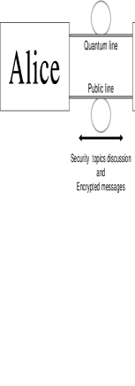
Figure 4.2: The setup of BB84 quantum key distribution protocol. The quantum line is used for the distribution of the key, while the classical line for discussing security topics and the transmission of encrypted messages.

4.1.1 The BB84 quantum key distribution protocol

Looking back in Figure 1.2, presented in page 1.2, one can see from the basic features of quantum mechanics that it is not easy for Eve to steal information, since it cannot be copied by no-cloning theorem. Moreover, it is impossible for her to distinguish non-orthogonal states, and any information gain related to such a distinction involves a disturbance. Then Alice and Bob by sacrificing some piece of information, and checking through the coincidence of their key can verify whether Eve was listening to them. Motivated by the above arguments Bennet and Brassard presented in 1984 the first quantum cryptographic protocol [32] described next.

Suppose Alice has an $n$-bit message. Then in order to generate an equal length cryptographic key she begins with some $a$ and $b$ $\left(4+\delta\right)n$-bit strings randomly produced. She must then encode this to a $\left(4+\delta\right)n$-qubit string

$$\left|\psi\right\rangle\equiv\bigotimes_{k=1}^{\left(4+\delta\right)n}\left|\psi_{a_{k}b_{k}}\right\rangle,$$

where $a_{k}$ the $k$-th bit of $a$ (and similarly for $b$), and each qubit just mentioned can be

$$\left|\psi_{00}\right\rangle \triangleq \left|0\right\rangle,$$ (4.1)

$$\left|\psi_{10}\right\rangle \triangleq \left|1\right\rangle,$$

$$\left|\psi_{01}\right\rangle \triangleq \left|+\right\rangle=\frac{\left|0\right\rangle+\left|1\right\rangle}{\sqrt{2}},$$

$$\left|\psi_{11}\right\rangle \triangleq \left|-\right\rangle=\frac{\left|0\right\rangle-\left|1\right\rangle}{\sqrt{2}},$$

where $\left|+\right\rangle$ is produced by application of the Hadamard gate on $\left|0\right\rangle,$ and $\left|-\right\rangle$ by applying the same gate on $\left|1\right\rangle.$ The above procedure, encodes $a,$ in the basis $\left\{\left|0\right\rangle,\left|1\right\rangle\right\}$ if $b_{k}=0,$ or in $\left\{\left|+\right\rangle,\left|-\right\rangle\right\}$ if $b_{k}=1.$ The states of each basis are not orthogonal to the ones of the other basis, and hence they cannot be distinguished, without distortion. $\delta$ is used as a tolerance due to noise of the channel.

The pure state $\left|\psi\right\rangle\left\langle\psi\right|$ is sent over the quantum channel, and Bob receives $\mathcal{E}\left(\left|\psi\right\rangle\left\langle\psi\right|\right).$ He announces the receipt in the public channel. At this stage Alice, Bob and Eve have each their own states, described by their own density matrices. Moreover Alice has not revealed $b$ during the transmission, and Eve has difficulty in identifying $a$ by measurement, since she does not know in which basis she should do it, and hence any trial to measure disturbs $\mathcal{E}\left(\left|\psi\right\rangle\left\langle\psi\right|\right).$ However $\mathcal{E}\left(\left|\psi\right\rangle\left\langle\psi\right|\right)\neq\left|\psi\right\rangle\left\langle\psi\right|$ in general, because the channel can be noisy. The above description implies that $a$ and $b$ should be completely random, because any ability of Eve to infer anything about these strings, would jeopardize the security of the protocol. Note that quantum mechanics offers a way of perfect random number generation, just by applying on $\left|0\right\rangle$ state, the Hadamard gate, one obtains $\frac{\left|0\right\rangle+\left|1\right\rangle}{\sqrt{2}},$ and after a measurement either $\left|0\right\rangle$ or $\left|1\right\rangle$ are returned with probability $p=\frac{1}{2}.$

In order to find their key Bob proceeds in measuring $\mathcal{E}\left(\left|\psi\right\rangle\left\langle\psi\right|\right)$ in the basis determined by a string $b^{\prime}$ he generated randomly too. This way he measures the qubits and finds some string $a^{\prime}$. After the end of his measurements he asks Alice, on the public channel, to inform him about $b.$ They then discard all bits $a_{m}$ and $a_{m}^{\prime}$ having $b_{m}\neq b_{m}^{\prime},$ since they measured them in different bases and hence are uncorrelated. It should be stressed that the public announcement of $b$ does not help Eve to infer anything about $a$ or $a^{\prime}.$

At this point they both have new keys $a_{\text{A}}^{\prime}$ and $a_{\text{B}}^{\prime}$ of statistically approximate length $2n,$ and Alice selects randomly $n$-bits and informs Bob publicly about their values. If they find that a number of qubits above a threshold $t,$ disagree then they stop the procedure and retry. In case of many failures there is definitely an invader and they should locate him. In case of success, there are some approximately $n$ bit strings $a_{\text{A}}^{\prime\prime}$ and $a_{\text{B}}^{\prime\prime},$ not communicated in public. Then if for example Alice wants to send a message $M,$ she encodes it, taking $E=M\oplus a_{\text{A}}^{\prime\prime},$ and send $E$ through the public channel. Then Bob decodes it by $M^{\prime}=E\oplus a_{\text{B}}^{\prime\prime}.$ The current keys, strings $a_{\text{A}}^{\prime\prime}$ and $a_{\text{B}}^{\prime\prime},$ should be discarded and not reused.

How can Alice’s key $a_{\text{A}}^{\prime\prime}$ be the same as Bob’s $a_{\text{B}}^{\prime\prime}$ in the case of a noisy channel which results $\mathcal{E}\left(\left|\psi\right\rangle\left\langle\psi\right|\right)\neq\left|\psi\right\rangle\left\langle\psi\right|$? This is the main topic of the next subsection.

4.1.2 Information reconciliation and privacy amplification

As anyone can assume, the communication over the noisy quantum channel is imperfect, $\mathcal{E}\left(\left|\psi\right\rangle\left\langle\psi\right|\right)\neq\left|\psi\right\rangle\left\langle\psi\right|$, and hence even if there was no interference by Eve in general $a_{\text{A}}^{\prime}\neq a_{\text{B}}^{\prime}.$ Alice and Bob should perform an error correction to get the same key $a^{\ast},$ by discussing over the public channel and revealing some string $g$ related to $a_{\text{A}}^{\prime}$ and $a_{\text{B}}^{\prime}.$ This is named information reconciliation. In order to have a secure key they should have privacy amplification by removing some bits of $a^{\ast}$ to get $a^{\prime\prime},$ minimizing Eve’s knowledge, since $a_{\text{A}}^{\ast}$ are related to string $g$ publicly communicated. It is known that both procedures can be used with high security.

As already seen information reconciliation is nothing more than error-correction; it turns out that privacy amplification it related to error-correction too, and both tasks are implemented using classical codes. To be more specific decoding from a randomly chosen CSS code, already presented in subsection 3.2.1, can be thought of as performing information reconciliation and privacy amplification. This can be seen by considering their classical properties. Consider two classical linear codes $C_{1}$ and $C_{2}$ which satisfy the conditions for a $t$ bit error-correcting $\left[n,m\right]$ CSS code. To perform the subsequent task the channel should sometimes randomly tested and seen to have errors less than $t,$ including eavesdropping.

Alice should pick randomly the codes $C_{1}$ and $C_{2}.$ Assume that $a_{\text{A}}^{\prime}=a_{\text{B}}^{\prime}+e,$ where $e$ is some error. Since it is known that less than $t$ errors occurred, if Alice and Bob both correct their states to the nearest codeword in $C_{1},$ their results will be $a^{\ast}.$ This step is information reconciliation. To reduce Eve’s knowledge Alice and Bob identify which of the $2^{m}$ cosets of $C_{2}$ in $C_{1}$ their state $a^{\ast}$ belongs to. This is done by computing the coset $a^{\ast}+C_{2}$ in $C_{1}.$ The result is their $m$ bit key sting $a^{\prime\prime}.$ By virtue of Eve’s knowledge about $C_{2},$ and the error-correcting properties of $C_{2}$, this procedure can reduce Eve’s mutual information with $a^{\prime\prime}$ to an acceptable level, performing privacy amplification.

4.1.3 Privacy and security

In order to quantify bounds in quantum cryptography, two important notions are defined in this subsection: privacy and security.

Assume Alice sends the quantum states $\rho_{k}^{A},$ $k=0,1,2,\ldots,$ and Bob receives $\rho_{k}^{B}=\mathcal{E}\left(\rho_{k}^{A}\right).$ The mutual information between the result of any measurement Bob may do and Alice’s value, $H\left(B:A\right),$ is bounded above by Holevo bound (2.6), thus $H\left(B:A\right)\leq\chi^{B},$ and similarly Eve’s mutual information is bounded above by $H\left(E:A\right)\leq\chi^{E}.$ Since any excess information Bob has relative to Eve, at least above a certain threshold can in principle be exploited by Bob and Alice to distill a shared secret key using the techniques of the last subsection. It makes sense to define privacy as

$$\mathcal{P}\triangleq\underset{\mathcal{S}}{\sup}\left[H\left(B:A\right)-H\left(E:A\right)\right],$$

where $\mathcal{S}$ are all the possible strategies Alice and Bob may employ to the channel. This is the maximum excess classical information that Bob may obtain relative to Eve about Alice’s quantum signal. Using the HSW theorem (3.10), Alice and Bob may employ a strategy such that $H\left(B:A\right)=\chi^{B},$ while for any strategy Eve may employ, $H\left(E:A\right)\leq\chi^{E}.$ Thus $\mathcal{P}\geq\chi^{B}-\chi^{E}.$ A lower bound may be obtained by assuming that Alice’s signal states are pure (refer to discussion after equation (3.10) to see why), $\rho^{A}=\left|\psi_{k}^{A}\right\rangle\left\langle\psi_{k}^{A}\right|,$ and if Eve initially had an unentangled state $\left|0^{E}\right\rangle,$ which may also assumed pure. Suppose Eve’s interaction is $\left|\psi^{EB}\right\rangle=U\left|\psi_{k}^{A}\right\rangle\left|0^{E}\right\rangle,$ since it is a pure state, the reduced density matrices $\rho_{k}^{E}$ and $\rho_{k}^{B}$ will have the same non-zero eigenvalues, and thus the same entropies, $S\left(\rho_{k}^{E}\right)=S\left(\rho_{k}^{B}\right).$ Thus $\mathcal{P}\geq\chi^{B}-\chi=S\left(\rho^{B}\right)-\sum_{k}p_{k}S\left(\rho_{k}^{B}\right)-S\left(\rho^{E}\right)+\sum_{k}p_{k}S\left(\rho_{k}^{E}\right)=S\left(\rho^{B}\right)-S\left(\rho^{E}\right)=I\left(\rho,\mathcal{E}\right),$ where the definition (2.10) was used. Note that the lower bound for privacy is protocol independent.

A quantum key distribution (QKD) protocol is defined secure if, for any security parameters $s>0$ and $l>0$ chosen by Alice and Bob, and for any eavesdropping strategy, either the scheme aborts, or succeeds with probability at least $1-O\left(2^{-s}\right),$ and guarantees that Eve’s mutual information with the final key is less than $2^{-l}.$ The key string must also be essentially random.

4.1.4 A provable secure version of the BB84 protocol

It can be proven [1, p.593-599] that using CSS codes one can have a 100% secure quantum key distribution. However CSS codes need perfect quantum computation, which is not yet achieved. Fortunately there is a chance of using the classical properties of CSS_u,v codes defined in (3.6) to have an equally secure classical computation version of BB84 protocol (refer to [1, p.599-602] for a proof). This version is made up of the following steps:

1. Alice creates $\left(4+\delta\right)n$ random bits.

2. For each bit, she creates a qubit either in the $\left\{\left|0\right\rangle,\left|1\right\rangle\right\}$ or in $\left\{\left|+\right\rangle,\left|-\right\rangle\right\}$ basis, according to a random bit string $b,$ see for example (4.1).

3. Alice sends the resulting qubits to Bob.

4. Alice chooses a random $v_{k}\in C_{1}.$

5. Bob receives the qubits, publicly announces this fact, and measures each in the $\left\{\left|0\right\rangle,\left|1\right\rangle\right\}$ or in $\left\{\left|+\right\rangle,\left|-\right\rangle\right\}$ basis randomly.

6. Alice announces $b.$

7. Alice and Bob discard those bits Bob measured in a basis other than $b.$ With high probability, there are at least $2n$ bits left; if not, abort the protocol. Alice decides randomly on a set of $2n$ bits to continue to use, randomly selects $n$ of these to check bits, and announces the selection.

8. Alice and Bob publicly compare their check bits. If more than $t$ of these disagree, they abort the protocol. Alice is left with the $n$ bit string $x,$ and Bob with $x+\epsilon.$

9. Alice announces $x-v_{k}.$ Bob subtracts this from his result, correcting it with code $C_{1}$ to obtain $v_{k}.$

10. Alice and Bob compute the coset of $v_{k}+C_{2}$ in $C_{1}$ to obtain the key $k.$

4.2 A commercial quantum cryptographic device

After a theoretical presentation of quantum key distribution it is time to present experimental results and then discuss the possibility of having a commercial device realizing quantum cryptography. These two topics are discussed correspondingly in subsections 4.2.1 and 4.2.2.

4.2.1 Experimental quantum key distribution

The first demonstration of quantum key distribution was performed at the IBM laboratory in 1989 [33] over a distance of 30 cm. Since then there has been remarkable improvement, demonstrating quantum key distribution over a distance of 10 km [34, 35], in IBM too, or over distances exceeding 40km, and also in installed telecommunication fiber, under the Lake Geneva [36].

In most cases experimental quantum cryptography is done using single photons, and optical fibers are used to guide them from Alice to Bob. Once the medium is chosen one should pick the right source and detectors. Since they have to be compatible, the crucial choice is the wave length. There are two main possibilities. Either one chooses a wavelength around 800 nm where efficient photon counters are commercially available, or one chooses a wavelength compatible with today’s telecommunication optical fibers, that is near 1300 nm or 1550 nm. The first choice requires the use of special fibers, hence the installed telecommunications networks can’t be used. The second choice requires the improvement or development of new detectors not based on silicon semiconductors which are transparent above 1000 nm wavelength. It is still unclear which of the two alternatives will turn out to be the best choice.

In what concerns the production of photons according to the BB84 states, defined in equation (4.1), one can choose different polarization states, which form non-orthogonal bases. Polarization can be for example linear, identifying $\left|0\right\rangle\equiv\left|\uparrow\right\rangle$ and $\left|1\right\rangle\equiv\left|\downarrow\right\rangle,$ or circular identifying $\left|+\right\rangle\equiv\left|\circlearrowleft\right\rangle$ and $\left|-\right\rangle\equiv\left|\circlearrowright\right\rangle.$ However in practice single photon states are difficult to realize thus approximately single photon states are produced by faint laser pulses.

Finally one should detect these approximate single photon states. This is achieved using a variety of techniques. One can choose between photomultipliers, avalanche-photodiodes, multichannel plates and supraconducting Josephson junctions.

A typical experimental setup for quantum key distribution, with the technology described above is sawn in Figure 4.3.

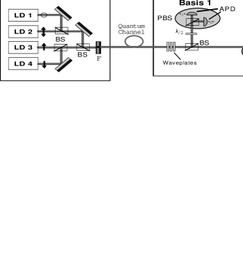
Figure 4.3: Typical system for quantum cryptography using polarization coding (LD: laser diode, BS: beamsplitter, F: neutral density filter, PBS: polarizing beam splitter, $\lambda/2$: half waveplate, APD: avalanche photodiode).

For more experimental details on the single photon quantum key distribution one should refer to [4, p.11-29].

4.2.2 Commercial quantum cryptography

Once the experimental setup of quantum key distribution has been performed, as discussed in subsection 4.2.1 and as sawn in Figures 4.3 and 4.2, one needs to follow the steps presented in subsection 4.1.4, in order to achieve perfectly secure quantum cryptography. Of course these steps are nothing but an algorithm, which can be analyzed and easily implemented into a program which can run on current technology computers. Moreover special controlling devices are needed in order to instruct the laser diodes, the beam splitters and get the result of the measurements from the avalanche photodiodes. Such hardware is already available in the market. One should not forget that a public connection is needed, like for example the internet. For this reason there exist patents [37], which can convert quantum cryptography from a laboratory experiment into a commercial product. Such a patent is discussed bellow.

One can reconstruct the steps of subsection 4.1.4 into the following computer program:

1. Alice’s computer creates $\left(4+\delta\right)n$ random bits, using an unknown to anybody else algorithm. (One can also use quantum techniques as discussed in the third paragraph of subsection 4.1.1)

2. For each bit, Alice’s computer triggers with a controller one of the four laser diodes, as shown in Figure 4.2, according to a random bit string $b.$

3. This way the light beams are sent to Bob’s site into an agreed beforehand rate.

4. Alice’s computer has already implemented the classical version of CSS codes, and then it picks up randomly a $v_{k}\in C_{1}.$

5. Bob’s computer instructs with a controller the beam splitter sawn in Figure 4.2 in which basis to measure the light beam. The selection should be according to a random algorithm. There should be a device returning the result of the measurement of the avalanche photodiodes to Bob’s computer. Bob’s computer announces the fact through an internet line to Alice’s computer.

6. Alice’s computer announces $b.$

7. Both computers discard those bits Bob’s measured in a basis other than $b.$ With high probability, there are at least $2n$ bits left; if not, abort the protocol. Alice’s computer decides randomly on a set of $2n$ bits to continue to use, randomly selects $n$ of these to check bits, and announces to Bob’s computer through internet.

8. Both computers compare through internet their check bits. If more than $t$ of these disagree, they abort the protocol. Alice’s computer is left with the $n$ bit string $x,$ and Bob’s with $x+\epsilon.$

9. Alice’s computer announces $x-v_{k}.$ Bob’s computer subtracts this from his result, correcting it with code $C_{1}$ to obtain $v_{k}.$

10. Both computer calculate the coset of $v_{k}+C_{2}$ in $C_{1}$ to obtain the key $k.$

Concluding it should be noted that what is very important about the above implementation, is that it is completely automatic and almost no human intervention is needed. Thus users can just write their messages, command the computers to send them securely and in the other side receive them. Automatic process is what makes such a device successfully commercial.

Summary

The most important tools and results of classical and quantum information theory, obtained in the present Individual Study Option, are summarized in the Figure S.1.

Information Theory Classical      Quantum Shannon entropy      Von Neumann entropy $H\left(X\right)=-\sum_{x}p_{x}\log p_{x}$      $S\left(\rho\right)=-$tr$\left(\rho\log\rho\right)$ Distinguishability and accessible information Letters always distinguishable    Holevo bound $N=\left|X\right|$    $H\left(X:Y\right)\leq S\left(\rho\right)-\underset{x}{\sum}p_{x}S\left(\rho_{x}\right)$    $\rho=\underset{x}{\sum}p_{x}\left(\rho_{x}\right)$ Information-theoretic relations Fano inequality   Quantum Fano inequality $H\left(p_{e}\right)+p_{e}\log\left(\left|X\right|-1\right)\geq H\left(X|Y\right)$   $H\left(F\left(\rho,E\right)\right)+\left(1-F\left(\rho,E\right)\right)\log\left(d^{2}-1\right)$   $\geq S\left(\rho,E\right)$ Mutual information   Coherent information $H\left(X:Y\right)=H\left(Y\right)-H\left(Y|X\right)$   $I\left(\rho,E\right)=S\left(E\left(\rho\right)\right)-S\left(\rho,E\right)$ Data processing inequality   Quantum data processing inequality $X\rightarrow Y\rightarrow Z$   $\rho\rightarrow\mathcal{E}_{1}\left(\rho\right)\rightarrow\left(\mathcal{E}_{2}\circ\mathcal{E}_{1}\right)\left(\rho\right)$ $H\left(X\right)\geq H\left(X:Y\right)\geq H\left(X:Z\right)$   $S\left(\rho\right)\geq I\left(\rho,\mathcal{E}_{1}\right)\geq I\left(\rho,\mathcal{E}_{2}\circ\mathcal{E}_{1}\right)$ Noiseless channel coding Shannon’s theorem   Schumacher’s theorem $n_{\text{bits}}=H\left(X\right)$   $n_{\text{qubits}}=S\left(\sum_{x}p_{x}\rho_{x}\right)$ Capacity of noisy channels for classical information Shannon’s noisy coding theorem Holevo-Schumacher-Westmoreland theorem $C\left(\mathcal{N}\right)=\underset{p\left(x\right)}{\max}\text{ }H\left(Y:X\right)$ $C^{\left(1\right)}\left(\mathcal{E}\right)=\underset{\left\{p_{j},\rho_{j}\right\}}{\max}\left[S\left(\rho^{\prime}\right)-\underset{x}{\sum}p_{x}S\left(\rho_{x}^{\prime}\right)\right]$ $\rho_{x}^{\prime}=\mathcal{E}\left(\rho_{x}\right),$ $\rho^{\prime}=\underset{x}{\sum}p_{x}\rho_{x}^{\prime}$

Figure S.1: Summary of classical and quantum information theory.

The most important results concerning quantum cryptography, are summarized in Figure (S.2).

Quantum Cryptography BB84 protocol, sends the following states $\bigotimes_{k=1}^{\left(4+\delta\right)n}\left|\psi_{a_{k}b_{k}}\right\rangle$ see (4.1) for definitions Privacy of a quantum channel $\mathcal{E}$ $\mathcal{P}\geq I\left(\rho,\mathcal{E}\right)$

Figure S.2: Summary of quantum cryptography.

Appendix A Omitted proofs

A.1 Special diagonal transformation of normal matrices

In this appendix it is going to be demonstrated that for a $d\times d$ normal matrix $A$, there exists a set of unitary matrices $U_{i}^{\left(A\right)},$ such that $\sum_{i=1}^{d}U_{i}^{\left(A\right)}AU_{i}^{\left(A\right)\dagger}=$tr$\left(A\right)I.$ Since $A$ is a normal matrix, by spectral decomposition theorem there exists a matrix $U^{\left(A\right)}$ such that $U^{\left(A\right)}AU^{\left(A\right)\dagger}$ is diagonal, and for this diagonal matrix there exists a unitary transformation $V_{i\leftrightarrow j}AV_{i\leftrightarrow j}^{\dagger}$ which interchanges the $i$-th diagonal element with the $j$-th.

To see this suppose $B$ is a $d\times d$ dimensional diagonal matrix, then the following matrix

$$\left(V_{i\leftrightarrow j}\right)_{kl}\triangleq\left\{\begin{array}[]{c}\delta_{kl},\text{ }k\text{ or }l\neq i,j\\ 1,\text{ }k=j\text{ and }l=i\\ 1,\text{ }k=i\text{ and }l=j\\ 0,\text{ else}\end{array}\right.,$$

can be used to exchange the $i$-th diagonal element with the $j$-th of $B.$ Following the next steps $V_{i\leftrightarrow j}$ is initially proven to be unitary

$$V_{i\leftrightarrow j}V_{i\leftrightarrow j}^{\dagger} = \sum_{l=1}^{d}\left(V_{i\leftrightarrow j}\right)_{kl}\left(V_{i\leftrightarrow j}^{\dagger}\right)_{ln}=\sum_{l=1}^{d}\left(V_{i\leftrightarrow j}\right)_{kl}\left(V_{i\leftrightarrow j}\right)_{nl}$$

$$= \sum_{l=1}^{d}\left(\begin{array}[]{c}\delta_{kl},\text{ }k\text{ or }l\neq i,j\\ 1,\text{ }k=j\text{ and }l=i\\ 1,\text{ }k=i\text{ and }l=j\\ 0,\text{ else}\end{array}\right)\left(\begin{array}[]{c}\delta_{nl},\text{ }n\text{ or }l\neq i,j\\ 1,\text{ }n=j\text{ and }l=i\\ 1,\text{ }n=i\text{ and }l=j\\ 0,\text{ else}\end{array}\right)$$

$$= \left(\begin{array}[]{c}\delta_{kn},\text{ }k\text{ or }n\neq i,j\\ 1,\text{ }k=j\text{ and }n=j\\ 1,\text{ }k=i\text{ and }n=i\\ 0,\text{ else}\end{array}\right)=\delta_{kn}=I.$$

The ability of $V_{i\leftrightarrow j}$ to exchange the diagonal elements of matrix $B=diag\left\{\ldots,b_{i},\ldots,b_{j},\ldots\right\}$ is exhibited by

$$V_{i\leftrightarrow j}BV_{i\leftrightarrow j}^{\dagger} = \sum_{l=1}^{d}\sum_{m=1}^{d}\left(V_{i\leftrightarrow j}\right)_{kl}B_{lm}\left(V_{i\leftrightarrow j}^{\dagger}\right)_{mn}=\sum_{l=1}^{d}\left(V_{i\leftrightarrow j}\right)_{kl}b_{l}\left(V_{i\leftrightarrow j}^{\dagger}\right)_{nl}$$

$$= \sum_{l=1}^{d}\left(\begin{array}[]{c}\delta_{kl},\text{ }k\text{ or }l\neq i,j\\ 1,\text{ }k=j\text{ and }l=i\\ 1,\text{ }k=i\text{ and }l=j\\ 0,\text{ else}\end{array}\right)b_{l}\left(\begin{array}[]{c}\delta_{nl},\text{ }n\text{ or }l\neq i,j\\ 1,\text{ }n=j\text{ and }l=i\\ 1,\text{ }n=i\text{ and }l=j\\ 0,\text{ else}\end{array}\right)$$

$$= \left(\begin{array}[]{c}b_{n}\delta_{kn},\text{ }k\neq i,j\text{ or }n\neq i,j\\ b_{i},\text{ }k=j\text{ and }n=j\\ b_{j},\text{ }k=i\text{ and }n=i\\ 0,\text{ else}\end{array}\right)=diag\left\{\ldots,b_{j},\ldots,b_{i},\ldots\right\}.$$

Defining now $V_{23\cdots d1}\triangleq V_{1\leftrightarrow 2}V_{2\leftrightarrow 3}\cdots V_{d-1\leftrightarrow d}V_{d\leftrightarrow 1},$ which is unitary matrix as a multiplication of unitary matrices, then $V_{23\cdots d1}U^{\left(A\right)}AU^{\left(A\right)\dagger}V_{23\cdots d1}^{\dagger}$ is a diagonal matrix where the in the first diagonal place is the second diagonal element of $A$, in the second diagonal place the third diagonal element of $A$, and so on until the final diagonal place where the first diagonal element of $A$ stands. The next display visualizes the similarity transformation $V_{23\cdots d1}$

$$\left[\begin{array}[]{ccccccc}a_{11}&&&&&&\\ &a_{22}&&&&&\\ &&&\ddots&&&\\ &&&&a_{\left(d-2\right)\left(d-2\right)}&&\\ &&&&&a_{\left(d-1\right)\left(d-1\right)}&\\ &&&&&&a_{dd}\end{array}\right]\overset{V_{23\cdots d1}}{\rightarrow}\left[\begin{array}[]{ccccccc}a_{22}&&&&&&\\ &a_{33}&&&&&\\ &&&\ddots&&&\\ &&&&a_{\left(d-1\right)\left(d-1\right)}&&\\ &&&&&a_{dd}&\\ &&&&&&a_{11}\end{array}\right].$$

Enumerating all the cyclic permutations of $\left(1,2,\ldots,d\right)$ with a number $i$ then the following unitary matrices are defined $U_{i}^{\left(A\right)}\triangleq V_{i}U^{\left(A\right)}.$ It is straightforward to verify that,

$$\sum_{i=1}^{d}U_{i}^{\left(A\right)}AU_{i}^{\left(A\right)\dagger} = \left[\begin{array}[]{cccc}a_{11}+a_{22}+\ldots+a_{dd}&&&\\ &a_{22}+a_{33}+\ldots+a_{11}&&\\ &&\ddots&\\ &&&a_{dd}+a_{11}+\ldots+a_{\left(d-1\right)\left(d-1\right)}\end{array}\right]$$

$$= \text{tr}\left(A\right)I.$$

A.2 Projective measurements are equivalent to an addition of unitary operations

Let $P$ be a projector and $Q\triangleq I-P$ the complementary projector, in this appendix it will be sawn that there exist unitary matrices $U_{1},$ $U_{2}$ and a probability $p$ such that for all $\rho$, $P\rho P+Q\rho Q=pU_{1}\rho U_{1}^{\dagger}+\left(1-p\right)U_{2}\rho U_{2}^{\dagger}.$ Choose $p\triangleq\frac{1}{2},$ $U_{1}\triangleq Q-P$ and $U_{2}\triangleq Q+P\triangleq I.$ It is obvious that $U_{1}U_{1}^{\dagger}=\left(Q-P\right)\left(Q-P\right)=QQ+QP-PQ-+PP=Q+0+P=I,$ and $U_{2}U_{2}^{\dagger}=II=I.$ Now it is easy to check that

$$\frac{1}{2}U_{1}\rho U_{1}^{\dagger}+\frac{1}{2}U_{2}\rho U_{2}^{\dagger} = \frac{1}{2}\left(Q-P\right)\rho\left(Q-P\right)+\frac{1}{2}\left(Q+P\right)\rho\left(Q+P\right)$$

$$= \frac{1}{2}\left(Q\rho Q-Q\rho P-P\rho Q+P\rho P\right)+\frac{1}{2}\left(Q\rho Q+Q\rho P+P\rho Q+P\rho P\right)$$

$$= P\rho P+Q\rho Q.$$

q.e.d. (Abbas Edalat contributed to this proof)

Appendix B Distance measures of information

B.1 Classical information distance: Hamming

The Hamming distance of two strings, is defined to be the number of places their bits are different. Assuming $a$ and $b$ are the two $n$-bit strings, and $a_{i}$ and $b_{i}$ are their $i$-th bits, one can write

$$d\left(a,b\right)\triangleq\sum_{i=1}^{n}\left|a_{i}-b_{i}\right|.$$

Very naturally, a Hamming sphere of center $c$ and radius $\delta,$ is defined as the set of stings which have distance from $c$ less or equal to $\delta$

$$\text{Sph}\left(c,\delta\right)\triangleq\left\{s:d\left(c,s\right)\leq\delta\right\}.$$

B.2 Quantum information distance: Fidelity

Fidelity is a measure of distance of two quantum states, defined by

$$F\left(\rho,\sigma\right)\triangleq\text{tr}\sqrt{\rho^{\frac{1}{2}}\sigma\rho^{\frac{1}{2}}}=\underset{\left|\psi\right\rangle,\left|\phi\right\rangle}{\max}\text{ }\left|\left\langle\psi|\phi\right\rangle\right|,$$

and used to determine how well a quantum channel preserves information. To do this the following function can be defined

$$F_{\text{min}}\left(\mathcal{E}\right)\triangleq\underset{\left|\psi\right\rangle}{\min}\text{ }F\left(\left|\psi\right\rangle,\mathcal{E}\left(\left|\psi\right\rangle\left\langle\psi\right|\right)\right).$$

where the quantum channel is simulated via the quantum operation $\mathcal{E}$, and the minimization is considered as the worst case of a quantum signal. Another interesting definition is

$$\bar{F}\triangleq\sum_{j}p_{j}F\left(\rho_{j},\mathcal{E}\left(\rho_{j}\right)\right)^{2},$$

named the ensemble average fidelity. Finally it is important to quantify, how much entanglement between $R$ and $Q,$ sent through a quantum channel $\mathcal{E}$ (a trace preserving operation), is preserved. This can be done by entanglement fidelity

$$F\left(\rho,\mathcal{E}\right)\triangleq F\left(RQ,R^{\prime}Q^{\prime}\right)^{2}=\left\langle RQ\right|\left[\left(\mathcal{I}_{R}\otimes\mathcal{E}\right)\left(\left|RQ\right\rangle\left\langle RQ\right|\right)\right]\left|RQ\right\rangle=\sum_{j}\left|\text{tr}\left(\rho E_{i}\right)\right|^{2},$$ (B.1)

where the primes are for the states after the application of $\mathcal{E}$, and $E_{i}$ are the operation elements of $\mathcal{E}$.

Bibliography

• [1] M. A. Nielsen and I. L. Chuang. Quantum computation and quantum information. Cambridge University Press, Cambridge (2000).
• [2] J. Preskill. Physics 229: Advanced Methods of Physics - Quantum Computation and Information. California Institute of Technology (1998). URL: http://www.theory.caltech.edu/people/preskill/ph229/
• [3] A. Steane. Quantum computing. arXive e-print (URL: http://www.arXiv.org) quant-ph/9708022 (submitted to Rev. Mod. Phys.) (1997).
• [4] N. Gisin, G. Ribordy, W. Tittel and H. Zbinden. Quantum cryptography. arXive e-print (URL: http://www.arXiv.org) quant-ph/0101098 (2001). (submitted to Rev. Mod. Phys.).
• [5] C. Cohen-Tannoudji, B. Diu and F. Laloë. Quantum Mechanics, Vol. I. John Wiley and Sons (1977).
• [6] A. M. Turing. On computable numbers, with an application to Entsheidungsproblem. Proc. Lond. Math. Soc. 2, 42: 230 (1936).
• [7] C. E. Shannon. A mathematical theory of communication. Bell System Tech. J., 27: 379-423, 623-656 (1948).
• [8] C. E. Shannon and A. D. Weaver. The Mathematical Theory of Communication. University of Illinois Press, Urbana (1949).
• [9] R. Landauer. Information is physical. Physics Today, 44(5): 22-29 (1991).
• [10] Y. Manin. Computable and Uncomputable (in Russian). Sovetskoye Radio, Moscow (1980).
• [11] P. Benioff. The computer as a physical system: A microscopic quantum mechanical Hamiltonian model of computers as represented by Turing machines. J. Stat. Phys., 21(5): 563-591 (1980).
• [12] R. P. Feynman. Simulating physics with computers. Int. J. Theor. Phys., 21: 467 (1982).
• [13] D. Deutsch. Quantum theory, the Church-Turing Principle and the universal quantum computer. Proc. R. Soc. Lond. A, 400: 97 (1985).
• [14] R. S. Ingarden and K. Urbanik. Information as a fundamental notion of statistical physics, Bull. Acad. Polon. Sci., Sér. math. astr. phys., 9: 313-316 (1961).
• [15] R. S. Ingarden and K. Urbanik. Quantum informational thermodynamics, Bull. Acad. Polon. Sci., Sér. math. astr. phys., 21: 281-304 (1962).
• [16] R. S. Ingarden. A simplified axiomatic definition of information, Bull. Acad. Polon. Sci., Sér. math. astr. phys., 11: 209-211 (1963).
• [17] R. S. Ingarden. Information theory and thermodynamics of light. Part I. Foundations of information theory, Fortchr. Phys., 12: 567-594 (1964).
• [18] R. S. Ingarden. Simplified axioms for information without probability, Prace Mat., 9: 273-282 (1965).
• [19] K. Urbanik. On the concept of information, Bull. Acad. Polon. Sci., Sér. math. astr. phys., 20: 887-890 (1972).
• [20] P. W. Shor. Algorithms for quantum computation: discrete logarithms and factoring. In Proceedings, 35${}^{\text{\emph{th}}}$ Annual Symposium on Fundamentals of Computer Science, IEEE Press, Los Alamitos, CA (1994).
• [21] P. W. Shor. Polynomial time algorithms for prime factorization and discrete logarithms on a quantum computer. SIAM J. Comput., 26(5): 1484-1509 (1997).
• [22] L. Grover. In Proc. 28${}^{\text{\emph{th}}}$ Annual ACM Symposium on the theory of Computation, pages 212-219, ACM Press, New York (1996).
• [23] L. Grover. Quantum mechanics helps in searching for a needle in a haystack. Phys. Rev. Lett., 79(2): 325 (1997). arXive e-print (URL: http://www.arXiv.org) quant-ph/9706033.
• [24] D. Dieks. Communication by EPR devices. Phys. Lett. A, 92(6): 271-272 (1982).
• [25] W. K. Wooters and W. H. Zurek. A single quantum cannot be cloned. Nature, 299: 802-803 (1982).
• [26] A. S. Holevo. Statistical problems in quantum physics. In Gisiro Maruyama and Jurii V. Prokhorov, editors, Proceedings of the Second Japan-USSR Symposium on Probability Theory, pages 104-119, Springer-Verlag, Berlin (1973).
• [27] B. Schumacher. Quantum coding. Phys. Rev. A, 51: 2738-2747 (1996).
• [28] A. R. Calderbank and P. W. Shor. Good quantum error-correcting codes exist. Phys. Rev. A, 54: 1098 (1996). arXive e-print (URL: http://www.arXiv.org) quant-ph/9512032.
• [29] A. Steane. Multiple particle interference and quantum error-correction. Proc. R. Soc. London A, 452: 2551-2576 (1996).
• [30] S. Singh. The Code Book. Fourth Estate Limited, London (1999).
• [31] R. L. Rivest, A. Shamir and L. M. Adleman. A method of obtaining digital signatures and public-key cryptosystems. Comm. ACM, 21(2): 120-126 (1978).
• [32] C. H. Bennett and G. Brassard. Quantum cryptography: Public key distribution and coin tossing. In Proceedings of IEEE International Conference on Computers, Systems and Signal Processing, pages 175-179, IEEE, New York (1984). Bangalore, India, December 1984.
• [33] C. H. Bennet, F. Bessette, G. Brassard, L. Salvail and J. Smolin. Experimental Quantum Cryptography. J. Cryptology, 5: 3-28 (1992).
• [34] D. S. Bethune and W. P. Risk. An autocompensating quantum key distribution system using polarization splitting of light. In IQEC’98 Digest of Postdeadline Papers, pages QPD12-2, Optical Society of America, Washington, DC (1998).
• [35] Donald S. Bethune and William P. Risk. An autocompensating fiber-optic quantum cryptography system based on polarization splitting of light. J. Quantum Electronics, 36(3): 100 (2000).
• [36] A. Muller, H. Zbinden and N. Gisin. Quantum cryptography over 23 km in installed under-lake telecom fibre. Europhys. Lett., 33: 334-339 (1996).
• [37] Y. Bakopoulos, Y. Vrettaros and A. Drigas. An Automatic Process for the Reliable and Secure Creation and Distribution of Quantum Keys. Pending patent submitted to Industrial Property Organization O.B.Y. Application number: 20010100204, dated: 19-4-2001, Athens (2001).