Qudit Quantum State Tomography

Abstract

Recently quantum tomography has been proposed as a fundamental tool for prototyping a few qubit quantum device. It allows the complete reconstruction of the state produced from a given input into the device. From this reconstructed density matrix, relevant quantum information quantities such as the degree of entanglement and entropy can be calculated. Generally orthogonal measurements have been discussed for this tomographic reconstruction. In this paper, we extend the tomographic reconstruction technique to two new regimes. First we show how non-orthogonal measurement allow the reconstruction of the state of the system provided the measurements span the Hilbert space. We then detail how quantum state tomography can be performed for multi qudits with a specific example illustrating how to achieve this in one and two qutrit systems.

I Introduction

With increasing interest in quantum computing, cryptography, and communication, it is of paramount importance that there exist means of benchmarking quantum information experiments. A singularly useful tool in this regard is Quantum State Tomography (QST), which provides a means of fully reconstructing the density matrix for a state. The procedure relies on the ability to reproduce a large number of identical states and perform a series of measurements on complimentary aspects of the state within an ensemble. The concept is not new, with the first such techniques developed by Stokes Stokes52a to determine the polarization state of a light beam. Recently James et al. James01a gave an extensive analysis of qubit systems specifically focusing on polarization entangled qubits, building on earlier experimental work White99a , but more generally for any number of qubits. We also refer the reader to Leonhardt‘s book Leonhardt97a which gives an introduction to some of the concepts and experimental techniques of tomography relating to continuous variable systems in modern quantum optics.

It is our aim here to expand on the work of James et al. in two ways: firstly, to detail how to perform QST on systems of $n$ qudits; secondly, to show how to perform QST when access to a full range of single qubit rotations and hence the state space is restricted. The first point is also motivated with respect to fundamental questions regarding non-locality in higher dimensions Kaszlikowski01a ; Collins01a as well as quantum information processing with improved security for Quantum key Distribution Brub01a ; Cerf01a and the need to characterize these larger quantum states. The second point provides a much larger cross-section of the physics community with the possibility of performing QST.

II 1 Qubit

To start with we will first introduce the Pauli operators using the group theoretical definition of them as generators. This is not crucial, though facilitates the procedure of going to higher dimensions with more subsystems without confusing notation changes. Hence, we can write a complete Hermitian operator basis for the qubit space:

$$\begin{array}[]{cc}I\equiv\hat{\lambda}_{0}=\left[\begin{array}[]{cc}1&0\\ 0&1\end{array}\right]&X\equiv\hat{\lambda}_{1}=\left[\begin{array}[]{cc}0&1\\ 1&0\end{array}\right]\\ \\ Y\equiv\hat{\lambda}_{2}=\left[\begin{array}[]{cc}0&-i\\ i&0\end{array}\right]&Z\equiv\hat{\lambda}_{3}=\left[\begin{array}[]{cc}1&0\\ 0&-1\end{array}\right],\end{array}$$ (12)

corresponding to the $2\times 2$ Identity operator, $\hat{\lambda}_{0}$, and the generators of the SU(2) group, $\hat{\lambda}_{j}$, $j$ = 1,2,3. The reason for denoting these with $\hat{\lambda}_{j}$ will become apparent as we go to higher dimensions. For a single qubit we can always write the density matrix as

$$\hat{\rho}_{2}=\frac{1}{2}\sum_{j=0}^{3}r_{j}\hat{\lambda}_{j},\;\;\;\;r_{j}\in\Re.$$ (13)

As the generators of SU(2) are all traceless operators, the normalization of the density matrix $\hat{\rho}_{2}$ requires $r_{0}$ set to one, leaving the other parameters $r_{j=1,\ldots,3}$ constrained only by $r_{1}^{2}+r_{2}^{2}+r_{3}^{2}\leq 1$. The terms, $r_{j}$, can be determined from the expectation value of the operators such that $r_{j}=\langle\hat{\lambda}_{j}\rangle={\rm Tr}[\hat{\rho}_{2}\hat{\lambda}_{j}]$. Thus the single qubit density matrix has the form,

$$\hat{\rho}_{2}=\frac{1}{2}\left[\begin{array}[]{cc}1+\langle\hat{\lambda}_{3}\rangle&\langle\hat{\lambda}_{1}\rangle-i\langle\hat{\lambda}_{2}\rangle\\ \langle\hat{\lambda}_{1}\rangle+i\langle\hat{\lambda}_{2}\rangle&1-\langle\hat{\lambda}_{3}\rangle\end{array}\right]$$ (16)

Theoretically, only three measurements are required to define the qubit density matrix. The fourth measurement, $\hat{\lambda}_{0}$, is practically necessary, as it allows renormalization of the count statistics to compensate for various experimental biases. The experimental data and the calculation of the expectation values $\langle\hat{\lambda}_{j}\rangle$ may lead to negative eigenvalues for the density matrix even though ${\rm Tr}\left[\hat{\rho}_{2}\right]=1$. This is due to the intrinsic uncertainty in experiments, however the mathematical expression (13) allows such nonphysical states (without the constraint $r_{1}^{2}+r_{2}^{2}+r_{3}^{2}\leq 1$ ). By using a maximally likelihood technique James01a , a physical density matrix can be derived.

We note that though the SU(2) generators described above do not correspond to any physical state, we can always write these operators in conjunction with the Identity $\hat{\lambda}_{0}$ as a linear combination of physical basis state density operators. In spin systems this Pauli group provides a perfectly reasonable set of observables, however in optics this is not the case. In optics a more common example could be the polarization basis,

$$\begin{array}[]{cc}|H\rangle\langle H|=\frac{1}{2}[\hat{\lambda}_{0}+\hat{\lambda}_{3}]&|V\rangle\langle V|=\frac{1}{2}[\hat{\lambda}_{0}-\hat{\lambda}_{3}]\\ |D\rangle\langle D|=\frac{1}{2}[\hat{\lambda}_{0}+\hat{\lambda}_{1}]&|L\rangle\langle L|=\frac{1}{2}[\hat{\lambda}_{0}-\hat{\lambda}_{2}]\end{array},$$ (19)

where, in the computational basis, $|H\rangle=|0\rangle$, $|V\rangle=|1\rangle$, $|D\rangle=[|0\rangle+|1\rangle]/\sqrt{2}$ and $|L\rangle=[|0\rangle+i|1\rangle]/\sqrt{2}$. The three orthogonal measurements are $|H\rangle,|D\rangle$ and $|L\rangle$ (depicted in Fig (1)).

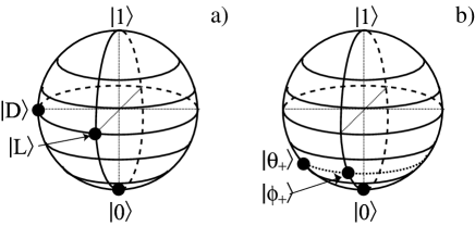
Figure 1: Schematic of measurements on the characteristic sphere (e.g. Poincaré or Bloch ) for qubit quantum state tomography In a), an orthogonal set of $|0\rangle,|D\rangle$ and $|L\rangle$ is shown while in b) a non-orthogonal set $|0\rangle,|\theta_{+}\rangle$ and $|\phi_{+}\rangle$ is shown.

Regardless of what orthogonal measurements we choose, we can always write $\hat{\lambda}_{j}=\sum_{k}a_{jk}\hat{\rho}_{k}$ for some other set of operators $\hat{\rho}_{k}$. State tomography may then be performed by measuring the expectation values $a_{jk}=\langle\hat{\rho}_{k}\rangle={\rm Tr}[\hat{\rho}_{2}\hat{\rho}_{k}]$.

II.1 Non orthogonal state tomography

In the state tomography that has been previously discussed we had assumed that we could measure observables at orthogonal points on the characteristic sphere. (For instance $|H\rangle,|D\rangle,|L\rangle$ in Fig (1).). In many practical situations the method of achieving these measurements could be a single qubit rotation followed by a measurement on $|0\rangle$, more explicitly, single qubit rotation would be necessary from $|0\rangle+|1\rangle$ and $|0\rangle+i|1\rangle$ to $|0\rangle$. One could envisage many practical situations where it is difficult to perform these large single qubit rotations to the $|0\rangle$ state. Does this mean that state tomography can not be performed? The answer is no, state tomography can also be performed if one has access only to a small solid angle on the characteristic sphere. For ideal measurements, one still needs to make a set of three measurements that project onto $|0\rangle$ and

$$|\theta_{+}\rangle=\frac{1}{\sqrt{2}}[\cos\theta|0\rangle + \sin\theta|1\rangle]$$ (20)

$$|\phi_{+}\rangle=\frac{1}{\sqrt{2}}[\cos\phi|0\rangle + i\sin\phi|1\rangle],$$ (21)

where $\theta,\phi$ can be small. Thus we only require a small perturbation about some accessible point on the characteristic sphere (see Fig(1b). This observation is likely to be important in experiments where qubit rotation is more demanding than measurement in the logical basis, such as flux qubit systems.

Naturally, as the measurement axes tend further away from orthogonal, the uncertainties for a fixed number of measurements will grow accordingly, or alternatively, achieving a target uncertainty in the state reconstruction will require a larger number of measurements.

Consider arbitrary states, $|\psi_{\nu}\rangle$, such that a projection measurement is represented by $\hat{\lambda_{\nu}}=|\psi_{\nu}\rangle\langle\psi_{\nu}|$. The count statistics arise from a series of these measurements. Correspondingly the average counts from a series of measurements will be

$$n_{\nu}={\cal N}\langle\psi_{\nu}|\hat{\rho}|\psi_{\nu}\rangle$$ (22)

where ${\cal N}$ is a constant that will be dependent on experimental factors such as detection efficiencies. The measured counts, $n_{\nu}$, are statistically independent Poissonian random variables and hence we assume that they will satisfy

$$\overline{\delta n_{\nu}\delta n_{\mu}}=n_{\nu}\delta_{\nu\mu}.$$ (23)

This now allows us to consider how these statistics will vary with respect to the nonorthogonal measurements.

The difference in count statistics when measuring with orthogonal states and when using nonorthogonal states will be proportional to the overlap of the two states Dieks88a . We now denote the measurement statistics resulting from projecting onto one of a set of nonorthogonal states, $|\psi_{\nu}^{\prime}\rangle$, as $n_{\nu}^{\prime}$. Hence we find that the counts for nonorthogonal measurements are related to the orthogonal in the following manner,

$$n_{\nu}^{\prime}={\cal N}|\langle\psi_{\nu}|\psi_{\nu}^{\prime}\rangle|^{2}\langle\psi_{\nu}|\hat{\rho}|\psi_{\nu}\rangle=n_{\nu}|\langle\psi_{\nu}|\psi_{\nu}^{\prime}\rangle|^{2}$$ (24)

with the errors appropriately scaled and given by

$$\overline{\delta n_{\nu}^{\prime}\delta n_{\mu}^{\prime}}=\frac{n_{\nu}\delta_{\nu\mu}}{|\langle\psi_{\nu}|\psi_{\nu}^{\prime}\rangle|^{2}}.$$ (25)

The counts and the errors all revert to the orthogonal case as $|\langle\psi_{\nu}|\psi_{\nu}^{\prime}\rangle|^{2}\rightarrow 1$.

III Generalization to qudits

We introduced the qubit tomography in terms of the SU(2) generators. Let us now consider a state with $d$ levels. Firstly we prepare the generators for SU($d$) systems and thereby construct the density matrices for a qudit system. For convenience we use the su algebra but we will denote the algebra for a $d$-dimensional system as su($d$). The generators of SU($d$) group may be conveniently constructed by the elementary matrices of $d$-dimension, $\{e^{k}_{j}|k,j=1\ldots d\}$. The elementary matrices are given by

$$(e^{k}_{j})_{\mu\nu}=\delta_{\nu j}\delta_{\mu k},\hskip 28.45274pt1\leq\nu,\mu\leq d,$$ (26)

which are matrices with one matrix element equal to unity and all others equal to zero. These matrices satisfy the commutation relation:

$$[e^{i}_{j},e^{k}_{l}]=\delta_{k,j}e^{i}_{l}-\delta_{il}e^{k}_{j}.$$ (27)

There are $d(d-1)$ traceless matrices,

$$\Theta_{j}^{k} = e^{k}_{j}+e^{j}_{k}$$ (28)

$$\beta_{j}^{k} = -i(e^{k}_{j}-e^{j}_{k}),\;\;\;1\leq k<j\leq d$$ (29)

which are the off-diagonal generators of the SU($d$) group. We add the $d-1$ traceless matrices

$$\eta_{r}^{r}=\sqrt{\frac{2}{r(r+1)}}\left[\sum_{j=1}^{r}e^{j}_{j}-re^{r+1}_{r+1}\right]$$ (30)

as the diagonal generators and obtain a total of $d^{2}-1$ generators. SU(2) generators are, for instance, given as $\{X=\Theta_{2}^{1}=e^{1}_{2}+e^{2}_{1},Y=\beta_{2}^{1}=-i(e^{1}_{2}-e^{2}_{1}),Z=\eta_{1}^{1}=e^{1}_{1}-e^{2}_{2}\}$.

We now define the $\lambda$-matrices, this is how we labelled the Pauli matrices in Eq.(12),

$$\lambda_{(j-1)^{2}+2(k-1)} = \Theta_{j}^{k}$$ (31)

$$\lambda_{(j-1)^{2}+2k-1} = \beta_{j}^{k}$$ (32)

$$\lambda_{j^{2}-1} = \eta_{j-1}^{j-1},$$ (33)

which, as shown previously, produce the $X,Y,Z$ operators of the SU(2) group and so on for higher dimensions. In conjunction with a scaled $d$-dimensional identity operator these form a complete hermitian operator basis.

It is then straightforward from Eq.(13) to see that a density matrix $\rho_{d}$ can be a linear combination of the generators as

$$\hat{\rho}_{d}=\frac{1}{d}\sum_{j=0}^{d^{2}-1}r_{j}\hat{\lambda}_{j}.$$ (34)

This $\rho_{d}$ is a density matrix of dimension $d$, a qudit, and the coefficient $r_{0}$ is one for the normalization. The condition ${\rm Tr}\left[\rho_{d}^{2}\right]\leq 1$ requires $\sum_{j=1}^{d^{2}-1}r_{j}^{2}\leq d(d-1)/2$.

Now let us extend these results to $n$-qudits. It was shown that for multiple qubits we only had to consider a space of operators defined by the tensor product of the generators, SU(2) $\otimes$ SU(2) $\otimes\ldots\otimes$ SU(2) where we have included $\lambda_{0}$ (the normalized identity matrix) with the normal SU(2) generatorsJames01a . For two qudits, a density matrix $\rho_{2\;d}$, which has dimension $d^{2}$, can be expanded similarly. All combinations of the tensor products of the $\lambda$-matrices (complimented with $\lambda_{0}$), $\lambda_{j1}\otimes\lambda_{j2}$, are linearly independent to each other. Hence, the expression of the density matrix $\rho_{2\;d}$ may be written in terms of $\lambda$-matrices,

$$\hat{\rho}_{2\;d}=\frac{1}{d^{2}}\sum_{j1,j2=0}^{d^{2}-1}r_{j1,j2}\hat{\lambda}_{j1}\otimes\hat{\lambda}_{j2}.$$ (35)

Similarly this expression can be generalized to density matrices of $n$ qudits, that is

$$\hat{\rho}_{nd}=\frac{1}{d^{n}}\sum_{j1\ldots jn=0}^{d^{2}-1}r_{j1\ldots jn}\hat{\lambda}_{j1}\otimes\ldots\otimes\hat{\lambda}_{jn}.$$ (36)

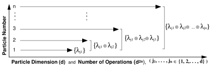
Figure 2: The measurement scaling for tomography on n-qudits results from the necessity to measure every basis state on every subsystem in every permutation. The measurements scale as $d^{2n}-1$ where $d$ is the particle dimension, e.g. $d=2$ for a qubit, and $n$ is the number of particles.

The tomography on such a state is only restricted by the patience of the experimentalist to determine the expectation values for the systems observables,

$$r_{j1\ldots jn}=\langle\hat{\lambda}_{j1}\otimes\ldots\otimes\hat{\lambda}_{jn}\rangle.$$ (37)

There will we $d^{2n}-1$ measurements required if we assume perfect detection. Fig.(2) illustrates the scaling catastrophe that occurs for multiple parties of higher-dimensional states. The key concept in both the extension to higher dimensional states and to more subsystems is that for each subsystem we need to measure every basis state on every subsystem in every permutation.

However if some structure is known about the state, then the number of measurements can be reduced. For example if we are confident that we are only ever dealing with a pure state then the number of measurements is significantly reduced and the scaling of measurements more so. QST for two qubits normally requires 15 measurements. If we know this state is pure this is reduced to 6: 3 on the diagonal; and 3 on the anti-diagonal. (In the case where we know the state to be, say, one of the Bell states, then this is reduced further to just 2). So in general for pure states we only require $2(d^{n}-1)$ measurements to reconstruct the density matrix.

The principle of nonorthogonal state tomography carries through to the higher dimensional cases in exactly the same way that it does for normal tomography using orthogonal states as do the considerations with respect to errors. Also a detailed discussion regarding the sources of error and there effect was outlined by James et al. James01a which was derived for the qubits but is equally valid for qudits by simple substitution and appropriate change in the summation ranges.

IV Qutrits

As a specific example of how we can implement higher dimension tomography consider a qutrit, $d=3$ dimensional, state. We can write this as

$$\hat{\rho}_{3}=\frac{1}{3}\sum_{j=0}^{8}r_{j}\hat{\lambda}_{j}$$ (38)

where the $\hat{\lambda}_{j}$ are now the SU(3) generators and an Identity operator $\hat{\lambda}_{0}$. For SU(3) the set of generators are

$$\begin{array}[]{cc}\hat{\lambda}_{1}=\left[\begin{array}[]{ccc}0&1&0\\ 1&0&0\\ 0&0&0\end{array}\right]&\hat{\lambda}_{2}=\left[\begin{array}[]{ccc}0&-i&0\\ i&0&0\\ 0&0&0\end{array}\right]\\ \\ \hat{\lambda}_{3}=\left[\begin{array}[]{ccc}1&0&0\\ 0&-1&0\\ 0&0&0\end{array}\right]&\hat{\lambda}_{4}=\left[\begin{array}[]{ccc}0&0&1\\ 0&0&0\\ 1&0&0\end{array}\right]\\ \\ \hat{\lambda}_{5}=\left[\begin{array}[]{ccc}0&0&-i\\ 0&0&0\\ i&0&0\end{array}\right]&\hat{\lambda}_{6}=\left[\begin{array}[]{ccc}0&0&0\\ 0&0&1\\ 0&1&0\end{array}\right]\\ \\ \hat{\lambda}_{7}=\left[\begin{array}[]{ccc}0&0&0\\ 0&0&-i\\ 0&i&0\end{array}\right]&\hat{\lambda}_{8}=\frac{1}{\sqrt{3}}\left[\begin{array}[]{ccc}1&0&0\\ 0&1&0\\ 0&0&-2\end{array}\right]\end{array}$$ (70)

which have been determined using the definitions of Eq.(31-33) and the corresponding elementary matrices of Eq.(26).

Once we have the expectation values for these operators then the density matrix can be reconstructed in the same way that it was done for the qubit in Eq.(16):

$$\hat{\rho}_{3}=\frac{1}{3}\left[\begin{array}[]{ccc}1+\frac{\sqrt{3}}{2}(\langle\hat{\lambda}_{8}\rangle+\sqrt{3}\langle\hat{\lambda}_{3}\rangle)&\frac{3}{2}(\langle\hat{\lambda}_{1}\rangle-i\langle\hat{\lambda}_{2}\rangle)&\frac{3}{2}(\langle\hat{\lambda}_{4}\rangle-i\langle\hat{\lambda}_{5}\rangle)\\ \frac{3}{2}(\langle\hat{\lambda}_{1}\rangle+i\langle\hat{\lambda}_{2}\rangle)&1+\frac{\sqrt{3}}{2}(\langle\hat{\lambda}_{8}\rangle-\sqrt{3}\langle\hat{\lambda}_{3}\rangle)&\frac{3}{2}(\langle\hat{\lambda}_{6}\rangle-i\langle\hat{\lambda}_{7}\rangle)\\ \frac{3}{2}(\langle\hat{\lambda}_{4}\rangle+i\langle\hat{\lambda}_{5}\rangle)&\frac{3}{2}(\langle\hat{\lambda}_{6}\rangle+i\langle\hat{\lambda}_{7}\rangle)&1-\sqrt{3}\langle\hat{\lambda}_{8}\rangle\end{array}\right]$$ (74)

The most direct way to do this is to measure the expectation values for the $\hat{\lambda}$-operators. However if this is not possible let us assume we can measure some set of basis states. Consider an arbitrary, but complete, set of basis states $\{|\psi_{i}\rangle\}$ with the associated projection operators $\{\hat{\mu}_{i}=|\psi_{i}\rangle\langle\psi_{i}|\}$. These can be linearly related, via a $d^{2}\times d^{2}$ matrix $A$, to the $\lambda$-matrices, $\hat{\mu}_{i}=\sum_{j}A_{i}^{j}\hat{\lambda}_{j}$. We can thus consider measurement outcomes,

$$n_{i}={\cal N}\langle\psi_{i}|\hat{\rho}|\psi_{i}\rangle = {\cal N}{\rm Tr}[\hat{\rho}\;\hat{\mu}_{i}]$$ (75)

$$= {\cal N}\sum_{j=0}^{8}A_{i}^{j}{\rm Tr}[\hat{\rho}\;\hat{\lambda}_{j}]$$

$$= {\cal N}\sum_{j=0}^{8}A_{i}^{j}r_{j},$$

where ${\cal N}$ is again a constant that will be dependent on experimental factors such as detection efficiencies. So we find, $r_{j}={\cal N}^{-1}\sum_{i=0}^{8}(A_{i}^{j})^{-1}n_{i}$, and finally,

$$\hat{\rho}_{3}={\cal N}^{-1}\sum_{i,j=0}^{8}(A_{i}^{j})^{-1}n_{i}\hat{\lambda}_{j}$$ (76)

In this way the state is reconstructed from the measurement outcomes in some arbitrary basis and the $A$-matrix which relates the measurement basis to the $\lambda$-matrices. This $A$-matrix will be invertible if a complete set of tomographic measurements are made, ie. if we measure in a complete basis. The $A$-matrix becomes the identity in the case where we use the generators.

Take a physical realization of a qutrit in an linear optics regime. Fig.(3) shows one way in which a qutrit may be realized KwiatJMO . The modes correspond to a photon taking the short medium or long paths of the interferometer. The values of the reflectivities of the beamsplitters are such that an even superposition state is generated. By varying the phases $\phi_{1}$ and $\phi_{2}$ a complete basis can be generated,

$$\begin{array}[]{cc}|0\rangle&|1\rangle\\ |0\rangle+1\rangle+2\rangle&\\ |0\rangle+\alpha|1\rangle+\alpha^{2}|2\rangle&\hskip 34.14322pt|0\rangle+\alpha^{2}|1\rangle+\alpha|2\rangle\\ |0\rangle+|1\rangle+\alpha|2\rangle&\hskip 28.45274pt|0\rangle+\alpha|1\rangle+|2\rangle\\ |0\rangle+|1\rangle+\alpha^{2}|2\rangle&\hskip 31.2982pt|0\rangle+\alpha^{2}|1\rangle+|2\rangle,\end{array}$$ (82)

where $\alpha=e^{2\pi i/3}$.

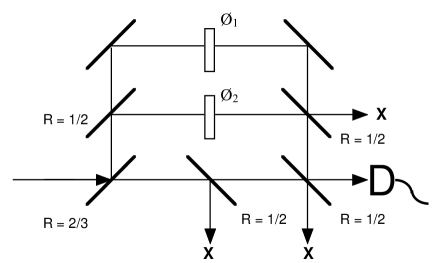
Figure 3: A linear optic implementation of a qutrit where the levels of the system are encoded in the pathlength travelled. The reflectivities for the beamsplitters, R, are given and the extra beamsplitter in the short arm effectively balances the superposition of the output. Phase elements in two of the arms provide the ability to consider any balanced superposition state in the qutrit space.

We can then utilize another 3-arm interferometer as that shown in Fig.(3) to rotate and perform projective measurements on the qutrit. Therefore one can perform a series of these projective measurements and, via the procedure outlined in Eq.(75-76), reconstruct the qutrit.

The same procedure applies regardless of the architecture provided we measure a complete set of states. To take another optical example, orbital angular momentum could be used to realize qutrits (and indeed, qudits), with holographic plates generating the qutrit superpositions and holographic interferometers acting as analyzers.

If we now further extend this to two qutrits, which may be entangled,

$$\hat{\rho}_{23}=\frac{1}{9}\sum_{j,k}r_{jk}\hat{\lambda}_{j}\otimes\hat{\lambda}_{k},$$ (83)

we can consider operators of the form $\hat{\lambda}_{j}\otimes\hat{\lambda}_{k}$, or linearly related operators,

$$\hat{\mu}_{i}\otimes\hat{\mu}_{j}=\sum_{k,l=0}^{8}A_{ij}^{kl}\hat{\lambda}_{k}\otimes\hat{\lambda}_{l},$$ (84)

where the $i,j$ label the rows and $k,l$ the columns of the $A$-matrix. There will now be $d^{2n}-1=80$ measurements to be made. Therefore, as we did for one qutrit, we can again consider the measurement outcomes for states of the form $\{|\psi_{i}\rangle\otimes|\psi_{j}\rangle=|\psi_{ij}\rangle\}$ with the associated projection operators $\{\hat{\mu}_{ij}=\hat{\mu}_{i}\otimes\hat{\mu}_{j}=|\psi_{ij}\rangle\langle\psi_{ij}|\}$.

$$n_{ij}={\cal N}\langle\psi_{ij}|\hat{\rho}|\psi_{ij}\rangle = {\cal N}{\rm Tr}[\hat{\rho}(\hat{\mu}_{i}\otimes\hat{\mu}_{j})]$$ (85)

$$= {\cal N}\sum_{k,l=0}^{8}A_{ij}^{kl}{\rm Tr}[\hat{\rho}\hat{\lambda}_{k}\otimes\hat{\lambda}_{l}]$$

$$= {\cal N}\sum_{k,l=0}^{8}A_{ij}^{kl}r_{kl}.$$

So we find, $r_{kl}={\cal N}^{-1}\sum_{i,j=0}^{8}(A_{ij}^{kl})^{-1}n_{ij}$, and finally,

$$\hat{\rho}_{23}={\cal N}^{-1}\sum_{i,j,k,l=0}(A_{ij}^{kl})^{-1}n_{ij}\hat{\lambda}_{k}\otimes\hat{\lambda}_{l}$$ (86)

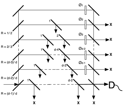
Figure 4: A state generation, or measurement, scheme for qudits using linear optical elements. The beamsplitter reflectivities and phases are in complete analogy to the description in Fig.(3) for the qutrit generation. For generation and measurement the number of elements scale as $d^{2}+3d$.

We can then reconstruct the density matrix for the state using the experimental measurement outcomes, $n_{i,j}$, and this $A$ matrix. Once we have the density matrix for the entangled qutrit state we can then consider questions of purity and entanglement. We refer the reader to Caves00a which gives a thorough exposition with respect to characterizing entangled qutrits that is of relevance to both pure and mixed states.

This change of basis is completely general and allows us to consider the reconstruction of any discrete system. We can now use: the generators; any orthonormal physical basis set; or, more importantly, in the case where we have limited access to the state space, a non-orthogonal basis.

As mentioned previously there is significant motivation to study entangled $d$-dimensional states and with the reconstruction of the complete density matrix many important state characteristics can be determined. In practice however, the dimensions will be restricted due to the complexity in implementing the measurements of the $d$-dimensional state.

In the case of generating a qudits using a linear optical elements the number of elements required to generate and hence also measure these higher dimensional states increases rapidly. Fig.(4) shows the general scaling for a system to generate qudits in a linear optics regime. For this implementation the state generation and measurement requires $d^{2}+3d$ elements for each qudit. The probability of producing these state scales as $(1/2)^{d-1}$ and similarly for its measurement. Similar complexity issues will be relevant regardless of the architecture.

V Conclusion

We have given a simple yet illustrative account of Quantum State Tomography for discrete systems, from a single qubit with an orthonormal measurement basis to multipartite-multidimensional systems with limited access to measurements in the Hilbert space. The specific example for the qutrit highlights the similarities and differences in going to higher dimensions whilst constructing an intuitive framework for the Quantum Information experimentalist to work. Primarily it is hoped that we have made QST relevant and accessible to a wider cross-section of the physics community. QST can provide a powerful tool for the experimentalist in QIS regardless of physical implementation, be it ion trap, quantum dot, flux qubit, or photon, to name but a few.

References

- (1) G. C. Stokes, Trans. Cambridge Philos. Soc. 9, 399 (1852).
- (2) D. F. V.James, P. G. Kwiat, W. J. Munro and A. G. White, Phys. Rev. A 64, 052312 (2001) .
- (3) A. G. White, D. F. V. James, P. H. Eberhard and P. G. Kwiat, Phys. Rev. Lett. 83, 3103 (1999).
- (4) U. Leonhardt, Measuring the Quantum state of Light, Cambridge University Press, (1997).
- (5) D. Kaszlikowski, L. C. Kwek, J.-L. Chen, M. Zukowski and C. H.Oh, quant-ph/0106010 (2001).
- (6) D. Collins, N. Gisin, N. Linden, S. Massar and S. Popescu, quant-ph/0106024 (2000).
- (7) D. Bru and C. Machiavello, quant-ph/0106126 (2001).
- (8) N. J. Cerf, M. Bourennane, A. Karlsson and N. Gisin, quant-ph/0107130 (2001).
- (9) C. M. Caves and G. J. Milburn, Optics Comm., 179, 439 (2000).
- (10) D. Dieks, Phys. Lett. A, 126, 303 (1988).
- (11) Interferometric schemes may also be used to generate qubits. See for example: P. G. Kwiat, J. R. Mitchell, P. D. D. Schwindt and A. G. White, Journal of Modern Optics 47, 257 (2000).