[
Fermionic entanglement in itinerant systems
Abstract
We study pairwise quantum entanglement in systems of fermions itinerant in a lattice from a second-quantized perspective. Entanglement in the grand-canonical ensemble is studied, both for energy eigenstates and for the thermal state. Relations between entanglement and superconducting correlations are discussed in a BCS-like model and for -pair superconductivity.
PACS numbers: 03.67.Lx, 03.65.Fd
]
I introduction
The concept of quantum entanglement [1] is believed to play an essential role in quantum information processing (QIP) [2]. As a consequence many efforts have been devoted to the characterization of entanglement [3]. The very definition of entanglement relies on the tensor product structure of the state-space of a composite quantum system. Unfortunately, due to quantum statistics, such a structure does not appear in an obvious fashion for systems of indistinguishable particles, i.e., bosons or fermions. Indeed for these systems, in view of the (anti)symmetrization postulate, one has to restrict to a subspace of the -fold tensor product of the single particle spaces. Such a subspace, e.g., the totally anti-symmetric one, has not a naturally selected tensor product structure. It turns out that the notion of entanglement is affected for systems of indistinguishable particles by some ambiguity.
Since it is of direct relevance to several implementation proposals for QIP e.g., quantum-dots based, this issue has been very recently addressed in the literature [4, 5, 6, 7, 8]. A quantum computation model was proposed[9] by using local fermionic modes (LFMs)– sites which can be either empty or occupied by a fermion. Moreover the use of quantum statistics for some QIP protocols have been analyzed [10].
Along the same line of realizing a bridge between quantum information science and conventional many-body theory it has been discussed entanglement in magnetic systems [11, 12, 13, 14, 15]. In particular entanglement in both the ground state [11, 12] and thermal state [13, 14, 15] of a spin-1/2 Heisenberg spin chain have been analyzed in the literature. In this situation the system state is given by the Gibb’s density operator where tr is the partition function, the system Hamiltonian, is Boltzmann’s constant which we henceforth will take equal to 1, and the temperature. As represents a thermal state, the entanglement in the state is called thermal entanglement[13]. Finally the intriguing issue of the relation between entanglement and quantum phase transition [16] have been addressed in a few quite recent papers [17, 18].
In this paper we will explore the relations between entanglement and (super)conducting correlations by following the spirit of Ref. [6]. It is important to stress that, due to the lack of measure of genuine many-body entanglement, we restrict us pairwise entanglement in this paper. Notice that in this approach the subsystems are given by modes and not by particles. This is therefore an essentially second-quantized approach [21].
In Sec. II basic definitions are given and the mapping scheme between LFMs and qubits introduced in [6] is briefly recalleed. In Sec. III the entanglement in both eigenstates and thermal state is studied for free fermions hopping in a lattice. In Sec. IV the relations between pairwise entanglement of and superconducting correlations are discussed for Two types of superconductivity, BCS-like superconductivity [19], and the so-called -pair superconductivity[20]. Sec. V contains the conclusions.
II Lattice Fermions
Let us start by recalling some basic facts about (spinless) fermions on a lattice. In the second-quantized picture the basic objects are the creation and annihilation operators and of -th LFM. They satisfy the canonical anti-commutation relations
| (1) |
The Hilbert space naturally associated to the LFMs, known as Fock space , is spanned by basis vectors
From the above occupation-number basis it should be evident that is isomorphic to the –qubit space. This is easily seen by defining the mapping [6]
| (2) |
where is the raising operator of -th qubit. This is an Hilbert-space isomorphism between and . By means of this identification one can discuss entanglement of fermions by studying the entanglement of qubits. Clearly this entanglement is strongly relative to the mapping (2) and it is by no means unique. By defining new fermionic modes by automorphisms of the algebra defined by Eq.(1) one gives rise to different mappings between and with an associated different entanglement. This simple fact is one of the manifestations of the relativity of entanglement [22].
It is useful to see how the mapping (2) looks on the operator algebra level. From the relation it follows that
| (3) |
where is the component of the usual Pauli matrices for -th qubit. This algebra isomorphism is quite well-known in the condensed matter literature and it referred to as the Jordan-Wigner transformation[23]. Notice that the inverse of Eq.(3) is given by . We see that, due to the non-local character of the mapping () even simple fermionic (spin) models can be transformed into non-trivial spin (fermionic) models. On the other hand the fermionic state like are clearly mapped by onto product qubit states.
It is important to keep in mind that, for charged and/or massive fermions, the Fock space is not the state-space of any physical system. Indeed, at variance with massless neutral particles, e.g., photons, only eigenstates of are allowed physical vectors and, for the same reason, only operators commuting with could be physical observables. This of course is nothing but a superselection rule, i.e., that does not allow for linear superposition of states corresponding to different charge/mass eigenvalues [24].
Despite the above considerations we notice that in some situations one is led to attribute to the whole Fock space some physical meaning. This happens for systems in a symmetry broken phase. For example in superconductivity and superfuidity the order parameter corresponds to an expectation value of an operator connecting different -sectors. It follows that the associated mean-field Hamiltonian does not commute with .
Of course one can argue that this kind of violation occurs on a level that has not any deep physical significance, after all the mean-field approach is just a variational one aimed to produce good approximation to physical expectation values. According to this view therefore the properties, e.g., entanglement, of the ansatz states should not to be taken too seriously. Nevertheless we think that this issue has some interest and the relations between pairwise entanglement and superconductivity will be provided before the section of conclusions.
III Itinerant systems
Let us now consider free spinless fermions in a lattice. The Hamiltonian is given by
| (4) |
with the periodic boundary condition. Here represents the hopping integral between sites and is the chemical potential.
It is known that the eigenvalue problem of can be solved by a discrete Fourier transformation (DFT)
| (5) |
where After the DFT, the Hamiltonian (4) becomes
| (6) |
where is the total fermion number operator. From Eq.(6), we immediately obtain the eigenvectors
| (7) | |||||
| (8) |
and the corresponding eigenvalues
| (9) |
Associated to the new fermionic modes there is a tensor product structure for the Fock space. The latter is defined by the mapping
| (10) |
Obviously since the eigenstates are products with respect the tensor product structure due to the entanglement in the eigenstates (8) is always zero. However entanglement, associated with map may exist in the eigenstates. For instance, the concurrence for any pair of fermions when . The corresponding eigenstates are called W states [25, 26, 14].
A Entanglement in the eigenstates
In order to make an analysis of the entanglement of our spinless fermions we will use the notion of concurrence [27], This is a simple measure for two qubits that allows to quantify the entanglement between any pair of fermions by our mapping.
We define the reduced density matrix associated to the first and second LFMs as End(C4). Note that the Hamiltonian is translation invariant, therefore entanglement between nearest-neighbor fermions are identical. Due to the fact that the reduced density matrix have the following form
| (11) |
The nonvanishing relevant matrix elements of are given by ( denotes the expectation value over ),
| (12) | |||||
| (13) | |||||
| (14) |
The concurrence of is then given by [11]
| (15) |
As the matrix elements and do not appear in the concurrence (15), their expressions are not given in this paper. From Eqs.(14) and (15) it follows that, in order to obtain the concurrence, we need to compute the correlation functions and and the mean fermionic number For the eigenstate , after direct calculations [28], we obtain
| (16) | |||||
| (17) | |||||
| (18) |
where is the filling and
| (19) |
By combining Eq. (15) and (18) one gets the concurrence between two LFMs,
| (21) | |||||
which is determined only the filling and the correlation function This latter quantity is obviously related to the “itinerancy” of the state, i.e., how fermions propagate. It follows that the concurrence (21) contains direct information about the conducting properties of the given quantum state.
From Eq.(21) one can directly see that there exists entanglement if the correlation function and the filling factor satisfy the equation . Then we obtain that there exists pairwise entanglement between two LFMs in the eigenstates if in the range . In the case of , , and therefore [25, 26, 14]. For this state is maximally entangled. A trivial case is , there is no entanglement at all. Now we consider the case , i.e, the lattice is fully filled. Now , and hence . For the half filling (), and Eq.(21) reduces to Then the entanglement exists if and only if .
Now we consider the ground-state of the system. It is obtained by filling the lowest single particle energy levels. By taking for simplicity odd one has From this definition it follows now we take the limit the resulting expression is given by
| (22) |
where we have used Moreover from the inequality it follows that the second argument of the function in Eq. (21) it is always non negative and we can get rid of the maximization. the concurrence then becomes
| (24) | |||||
in the infinite lattice. Fig. 1 shows the concurrence as a function of the filling in the infinite lattice. We see that the entanglement becomes maximal at half filling for two neighboring fermions, and the entanglement is symmetric with respect to the point of half filling. At the point of half filling the concurrence simply becomes The property of symmetry can also be seen directly from Eq.(24) as the concurrence is invariant if we make the transformation .
For zero chemical potential i.e., half-filling , it exists a direct relation between the concurrence and the ground state energy density . Indeed from translational symmetry of the hamiltonian one has where we have used even the reality of This relation, that can be extend to finite temperature as well, is in a sense remarkable in that it connects entanglement with a thermodynamical quantity that depends on just the partition function of system. The latter is determined just by the Hamiltonian spectrum, whereas computing concurrence requires in general also the knowledge of the eigenstate. This kind of connection between entanglement and thermodynamical quantities has been discussed even for spin chains, both zero [connor01] and finite temperature [30].
B Thermal Entanglement
In this section we extend our analysis to the entanglement in a finite temperature. The state of fermions at thermal equilibrium is described by the following Gibbs gran-canonical state
| (25) |
where , is the Boltzman’s constant, and the partition function is given by
| (26) |
The average accupation numbers is given by
| (27) |
which is the Fermi-Dirac distribution. The expecation value is then easily obtained as
The reduced density matrix associated with will be a diagonal matrix. Then from Eq.(15), the concurrence is zero for any pair of LFMs. So we will discuss the entanglement associated to the map . The form of the reduced density matrix in the state is then given by Eq.(11) and the concurrence is given by Eq.(15). Now we need to calculate the correlation functions in Eq. (14) for the state The result is readily obtained from Eq. (18) by replacing the eigenvalues of the ’s with the corresponding thermal averages:
| (28) | |||||
| (29) |
Then the exact expression for the concurrence is given by the combination of Eqs.(14), (15), and (29). Note the concurrence is thus obtained in an analytical form for arbitrary To exemplify this result let us first consider the simple case of For two sites, from Eqs.(14), (15), and (29), the concurrence is given by
| (30) |
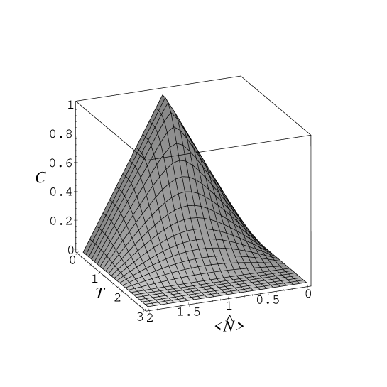
which is similar to the concurrence in a thermal state of the two-qubit model [14]. For three special values of , we have table I, from which we see that there is no entanglement when the chemical potential is (the corresponding mean fermion number is 0 and 2). The entanglement is maximal when and other parameters are fixed. The mean fermion number is simply given by
| (31) |
from which we obtain From this relation and Eq. (30) one can calculate the concurrence as a function of temperature and the mean fermion number This function is represented in Fig.2. We observe that the entanglement becomes maximal when the mean fermion number is 1 for fixed temperature . Let us first comment on the or in view of Eq.(30) equivalently symmetry of the function . This fact can be understood from Eq.(15). Clearly the only thing to check is that This latter statement easily follows by the use of particle-hole transformation i.e., realizing along with the unitary mapping that, for bi-partite lattices, changes the sign of Another important feature is the existence of a threshold temperature, after which the entanglement disappears. Remarkably this threshold temperature is independent of the mean fermion number. This phenomenon is related to the independence on an external magnetic field displayed by the associated spin model [13, 14].
For large , we plotted in Fig. 3 the concurrence as a function of temperature for different . We observe that the threshold temperature is independent of . Moreover it is worth noticing that, for sufficiently high ,i.e, filling, one has a non monotonic behavior of the concurrence as a function of . Indeed we see that the entanglement can initially increase as the temperature is raised. This phenomenon is due to the fact that the chemical potential in fermionic systems plays a role analogous to the external magnetic field for spin systems [13]. When is large enough the ground state is given by a product state (all the spins aligned), hence entanglement in the thermal state is due to the excited eigenstates. Of course for large enough one always gets in t hat the Gibbs state is approaching the maximally mixed state.
IV Entanglement and superconductivity
In this section we discuss fermionic entanglement in simple superconducting systems and explore the relations between entanglement and superconducting correlations. Let us first consider a BCS-like i.e., mean-field, model
A BCS-like superconductivity
The following BCS-like Hamiltonian describes the pairing between fermions carrying momentum and ,
| (32) |
The quantities are order parameters of conductor-superconductor phase transitions. They are determined by the self-consistent relations . and above a critical temperature they vanish thus signaling the absence of superconducting correlation.
The structure of Eq. (32) clearly suggest that the relevant tensor-product structure of this problem is given by where Moreover it is very simple to check that, for any the operators span a Lie-algebra. The states realize a spin- representation of such an algebra. Therefore the Hamiltonian (32), that it is equivalent to a spin-1/2 particle in an external magnetic field along the direction, is readily diagonalized. For example, if we define the ground state is given by where
| (33) |
It corresponds to the eigenvalue . Here The self-consistent equation for the ’s reads
| (34) |
The concurrence associated to the thermal state is given by
| (35) |
In the limit of , the concurrence becomes which is just the concurrence of the ground state . By solving these equations the numerical results are given in Fig.4. One can see that the concurrence goes to zero at a temperature slightly lower than superconductor critical one. Since in the temperature range the function is invertible one can express the concurrence as a function of the order parameter only. This is illustrated in Fig. 5 which shows that it is necessary to have a certain amount of superconducting correlation in order to have an pairwise entangled thermal state. Notice that we set that in a grand-canonical picture ( corresponds to half-filling [29].
We would like to observe now that a non mean-field Hamiltonian formally analogous to (32) plays an important role in the excitonic proposal for QIP by Biolatti et al [31]. In that case the fermionic bilinear terms are replaced by where () creates an electron (hole) in the -th (-th) state of the conduction (valence) band of a semiconductor. The order parameter becomes a (independently controllable) coupling to an external laser field. The excitonic index can be associated to different, spatially separated, quantum dots; this implies that Let denotes the particle-hole vacuum (ground state of the semiconductor crystal). Since one immediately sees that the “excitonic Fock space” span is isomorphic to a qubit space [21]. This example shows that one can consider spaces allowing for a varying number of “particles” that nevertheless are fully legitimate quantum state-spaces. No super-selection rule violation (possibly due to spontaneous symmetry-breaking) has to be invoked. Next we consider another kind of , non mean-field superconductivity, i.e., the -pair superconductivity.
B -pair superconductivity
Yang[20] discovered a class of eigenstates of the Hubbard model which have the property of off-diagonal long-range order (ODLRO)[32], which in turn implies the Meissner effect and flux quantization [33]. Let us begin by introducing the -operators
| (36) |
which form the su(2) algebra and satisfies Here the fermions have spins and the operator . The operators also satisfy the relations which reflect the Pauli principle, i.e., the impossibility of occupying a given site by more than one pair
In this context the relevant state-space is the one spanned by the basis vectors
| (37) |
From the above basis it is evident that the space span is isomorphic to the –qubit space. This is easily seen by defining the mapping
| (38) |
Then we can produce ‘number’ state by applying successive powers of on the vacuum state defined by So
| (39) |
where The span of the ’s ( known as -paired states, forms an irreducible spin- representation space. A mentioned above what makes the number states interesting is the fact that they have been shown to have ODLRO. Indeed from Eq.(39) the following, distance independent, correlation function is obtained
| (40) |
In the thermodynamical limit ( with ) goes like to , which is nonvanishing as In other words the number state exhinits ODLRO, and thus is superconducting.
The two-site reduced density matrix has the form (11) in which
| (41) | |||||
| (42) |
From these relations and Eq. (15) one finds
| (43) |
Notice that the formula above could have been directly obtained from Ref ([15]) where the entanglement between any pair of qubits in a Dicke state has been computed. Indeed by means of the the mapping (38), one can identify the number state with the usual Dicke state
In the thermodynamical limit one has thus, from Eq. (15) the entanglement becomes zero. So we see that the pairwise quantum entanglement does not exists although we have -pairing superconductivity in the number state. We finally notice that in the -pair coherent states discussed in [34], there is ODLRO, but being a products there obviously no entanglement.
V Conclusions
The Fock space of many local fermionic modes can be mapped isomorphically onto a many-qubit space. Using such a mapping we studied entanglement between pairs of (spinless) fermionic modes. This has been done both for the eigenstates and the thermal state for a model of free fermions hopping in a lattice (entanglement between local modes as function of temperature and filling). In the free fermionic model we analysed entanglement between local modes as function of temperature and filling. In particular we found that above a threshold temperature the thermal state becomes separable.
We studied the relations between pairwise entanglement and the superconducting correlation in both the BCS-like model and the -pair superconductivity. For the BCS-model, that a finite value of the superconducting order parameter is required to obtain entanglement in the thermal state. Notice that this last statement establishes a direct connection bewteen quantum entanglement and a real phase transition [35]. For -pair superconductivity we found that pairwise entanglement is not a necessary condition for the superconductivity.
Despite their simplicity, our results seem to suggest that the quantum information-theoretic relevant notion of quantum entanglement can provide useful physical insights in the physics of many-body systems of indistinguishable particles.
ACKNOWLEDGMENTS
We thank D Lidar for useful comments. This work has been supported by the European Community through the grant IST-1999-10596 ( Q-ACTA).
REFERENCES
- [1] E. Schrödinger, Naturwissenschaften 23, 809 (1935).
- [2] For reviews, see A. Steane, Rep. Prog. Phys. 61, 117 (1998); D. P. DiVincenzo and C. H. Bennett, Nature 404, 247 (2000).
- [3] For a review, see M. Horodecki, P. Horodecki, and R. Horodecki, in Quantum Information–Basic Concepts and Experiments, edited by G. Alber and M. Weiner (Springer, Berlin, in press).
- [4] J. Schliemann, D. Loss, and A. H. MacDonald, Phys. Rev. B 63, 085311 (2001); J. Schliemann, J. I. Cirac, M. Kuś, M. Lewenstein, and D. Loss, Phys. Rev. A 64, 022303 (2001).
- [5] Y. S. Li, B. Zeng, X. S. Liu and G. L. Long, Phys. Rev. A 64, 054302 (2001).
- [6] P. Zanardi, Phys. Rev. A (2002), in press, quant-ph/0104114.
- [7] R. Paškauskas and L. You, Phys. Rev. A 64, 042310 (2001).
- [8] J. Gittings, A. Fisher, quant-ph/0202051
- [9] D. S. Abrams and S. Lloyd, Phys. Rev. Lett. 79, 2586 (1997); S. B. Bravyi and A. Yu. Kitaev, quant-ph/0003137.
- [10] N. Paunkovic, Y. Omar, S. Bose, and V. Vedral, quant-ph/0112004; Y. Omar, N. Paunkovic, S. Bose, V. Vedral, quant-ph/0105120.
- [11] K. M. O’Connor and W. K. Wootters, 63, 0520302 (2001).
- [12] D. A. Meyer and N. R. Wallach, quant-ph/0108104.
- [13] M. A. Nielsen, Ph. D thesis, University of Mexico, 1998, quant-ph/0011036; M. C. Arnesen et al., Phys. Rev. Lett. 87, 017901 (2001).
- [14] X. Wang, Phys. Rev. A 64, 012313 (2001); X. Wang, H. Fu and A. I. Solomon, J. Phys. A: Math. Gen. 34,11307(2001);
- [15] X. Wang and K. Mølmer, Euro. Phys. J. D. , in press.
- [16] S. Sachdev, Quantum Phase Transitions, (Cambridge University Press, Cambridge, 2000).
- [17] T. J. Osborne and M. A. Nielsen, quant-ph/0109024, quant-ph/0202162
- [18] A. Osterloh et al. , quant-ph/0202029.
- [19] J. Bardeen, L. N. Cooper and J. R. Schrieffer, Phys. Rev. 108, 1175 (1957).
- [20] C. N. Yang, Phys. Rev. Lett. 63, 2144 (1989); C. N. Yang and S. C. Zhang, Mod. Phys. Lett. B 4, 759 (1990).
- [21] For a related analysis see also L. A. Wu and D. Lidar, quant-ph/0109078.
- [22] P. Zanardi, Phys. Rev. Lett. 87,077901 (2001).
- [23] P. Jordan and E. Wigner, Z. Phys. 47, 631 (1928).
- [24] See for example D. Giulini, Lect. Notes Phys. 559, 67(2000), quant-ph/0010090.
- [25] M. Koashi, V. Bužek, and N. Imoto, Phys. Rev. A 62, 050302(R)(2000).
- [26] W. Dür, G. Vidal, and J. I. Cirac, Phys. Rev. A 62, 062314 (2000).
- [27] S. Hill and W. K. Wootters, Phys. Rev. Lett. 78, 5022 (1997); W. K. Wootters, ibid. 80, 2245 (1998).
- [28] From Eqs.(5) we can express the operators and in terms of Fourier fermionic creation and annihilation operators. Then the relation Where the averages are taken in the eigenstate
- [29] This is immediately seen from the equation Tr
- [30] X.G. Wang, P. Zanardi, quant-ph/0202108
- [31] E. Biolatti, R. C. Iotti, P. Zanardi, and F. Rossi, Phys. Rev. Lett. 85 5647 (2000); Biolatti, I. D’Amico, P. Zanardi, F. Rossi, Phys Rev. B 65, 075306 (2002)
- [32] C. N. Yang, Rev. Mod. Phys. 34, 694 (1962).
- [33] G. L. Sewell, J. Stat. Phys. 61, 415 (1995); H. T. Nieh, G. Su, and B. M. Zhao, Phys. Rev. B 51, 3760 (1995).
- [34] A. Solomon and K. Penson, J. Phys. A: Math. Gen. 31, 355 (1998).
- [35] D. Aharonov, quant-ph/9910081.