$U(2)$ invariant squeezing properties of pair coherent states

Abstract

The $U(2)\/$ invariant approach is delineated for the pair coherent states to explore their squeezing properties. This approach is useful for a complete analysis of the squeezing properties of these two-mode states. We use the maximally compact subgroup $U(2)\/$ of $Sp(4,R)\/$ to mix the modes, thus allowing us to search over all possible quadratures for squeezing. The variance matrix for the pair coherent states turns out to be analytically diagonalisable, giving us a handle over its least eigenvalue, through which we are able to pin down the squeezing properties of these states. In order to explicitly demonstrate the role played by $U(2)\/$ transformations, we connect our results to the previous analysis of squeezing for the pair coherent states.

I Introduction

Pair coherent states (originally discussed for the case of charged bosons [3]) provide an interesting example of non-classical states of the two-mode radiation field [1, 2]. They have been studied in detail for their non-classical properties and as examples of EPR states [1, 2, 4, 5, 6, 7]. More recently, their experimental signatures have been explored [8].

Squeezing is an important signature of nonclassicality. By definition, when the noise in some quadrature of a quantum state falls below the coherent state value of $\hbar/2\/$, the state is squeezed and thus non-classical [9, 10]. The canonical commutation relations which lead to the uncertainty principle are fundamental to the analysis of squeezing. The linear canonical transformations of quadrature operators, under which the canonical commutation relations of the two-mode field are invariant, form a non-compact group $Sp(4,R)\/$. The group $Sp(4,R)\/$ acts on the quantum states of two-mode fields through the unitary representation of its double cover and represents the action of all possible quadratic Hamiltonians which are physically important [13]. The group $Sp(4,R)\/$ has a passive, photon number conserving, maximally compact subgroup $U(2)\/$ which acts on the creation and annihilation operators through its defining representation. The non-compact part of $Sp(4,R)\/$, while acting through its unitary representation on “classical” non-squeezed states can generate “non-classical” squeezed states. On the other hand, the compact $U(2)\/$ subgroup of $Sp(4,R)\/$ through its unitary action in the Hilbert space cannot generate non-classical states from classical ones. In particular it cannot generate a squeezed state starting from a non-squeezed state. Therefore, one can allow a state to undergo such a passive transformation before analysing any non-classical property [13, 14]. This maximally compact subgroup $U(2)\/$ of $Sp(4,R)\/$ while acting on the quadrature operators, allows us to search over all possible allowed quadratures for the two-mode fields [13]. This search enables one to locate the most squeezed quadrature. Thus the group $U(2)\/$ facilitates the analysis of quadrature squeezing and allows one to arrive at a $U(2)\/$ invariant description of squeezing. It is possible to generalize this analysis for the case of n-mode fields where the maximally compact subgroup of canonical transformations is $U(n)\/$ [15]

In this paper, we analyse the squeezing properties of pair coherent states using the $U(2)\/$ invariant methodology. It turns out that for these states the variance matrix (the matrix of all second order noise moments) has an interesting form. We are able to diagonalise it analytically through a series of orthogonal transformations, thus locating its spectrum and hence the smallest eigenvalue. The spectrum is invariant is under $O(4)\/$ and hence also under $U(2)$ transformations. Whenever this $U(2)\/$ invariant least eigenvalue is less than $\frac{1}{2}\/$ the state is squeezed. Further, we show that the orthogonal $O(4)\/$ matrix which diagonalises the variance matrix for these states lies outside the compact canonical transformations (the subgroup $U(2)\/$). Therefore, the pair coherent states provide an interesting example of states for which the variance matrix cannot be diagonalised within $O(4)\cap Sp(4,R)\/$, though we are able to bring the smallest eigenvalue to the leading diagonal position by some compact canonical transformations ($O(4)\/\cap\/Sp(4,R)\/$). Lastly we connect our results to the previous analysis on the squeezing properties of pair coherent states by Agarwal et. al. [1, 2]

The material in this paper is arranged as follows: in section II we describe the $U(2)\/$ invariant squeezing criterion and elaborate on the role played by $U(2)\/$ in the analysis of the non-classical properties of the two-mode fields. In section III we analyse the pair coherent states for their $U(2)\/$ invariant squeezing properties and section IV contains a few concluding remarks.

II $U(2)\/$ Invariant Squeezing

We consider two orthogonal modes of the radiation field, with annihilation operators $a_{1}\/$ and $a_{2}\/$. To handle the analysis of the two-mode fields compactly we introduce the column vectors

$$\xi^{(c)}\equiv\left(\xi_{a}^{(c)}\right)=\left(\begin{array}[]{c}a_{1}\\ a_{2}\\ a^{\dagger}_{1}\\ a^{\dagger}_{2}\end{array}\right),\quad\quad\xi\equiv\left(\xi_{a}\right)=\left(\begin{array}[]{c}q_{1}\\ q_{2}\\ p_{1}\\ p_{2}\end{array}\right).$$ (1)

$\xi^{(c)}\/$ being the vector of creation and annihilation operators and $\xi\/$ the vector of the quadrature operators, with their components having the usual relation, $q_{j}=\frac{1}{\sqrt{2}}\left(a_{j}+a_{j}^{\dagger}\right)$ and $p_{j}=\frac{-i}{\sqrt{2}}\left(a_{j}-a_{j}^{\dagger}\right)$. The canonical commutation relations can be written compactly in terms of these column vectors:

$$\begin{array}[]{ccc}\mbox{}\left[\xi^{(c)}_{a},\xi^{(c)}_{b}\right]&=&\beta_{ab}\\ &&\\ \mbox{}\left[\,\xi_{a},\xi_{b}\,\right]&=&i\beta_{ab}\end{array}\,\mbox{with}\quad\,\left(\beta_{ab}\right)=\left(\begin{array}[]{rrcc}\!\!0&\!\!\!\!0&1&0\\ \!\!0&\!\!0&0&1\\ \!\!-1&\!\!0&0&0\\ \!\!0&\!\!-1&0&0\end{array}\right)$$ (2)

The linear canonical transformations of the quadrature operators $q_{j}\/$ and $p_{j}\/$ are those real linear transformations that preserve the commutation relations given in equation (2). They constitute the four-dimensional symplectic group $Sp(4,R)$:

$$\xi\longrightarrow\xi^{\prime}=S\,\xi\/,\quad\quad S\in Sp(4,R)$$ (3)

$$Sp(4,R)=\left\{S=4\times 4\mbox{ real matrix }\,\,|\,\,S\/\beta\/S^{T}=\beta\right\}$$ (4)

The maximally compact subgroup $K=U(2)\/$ of $Sp(4,R)\/$, which is central to our analysis of squeezing, can be identified as:

$$K=\left\{S(X,Y)\in Sp(4,R)\,\,|\,\,U=X-iY\in U(2)\right\}$$ (5)

$$S(X,Y)=\left[\begin{array}[]{rl}X&Y\\ -Y&X\end{array}\right]$$ (8)

The action of this subgroup on the creation and annihilation operators is through its defining representation:

$$\left[\begin{array}[]{cc}a_{1}^{\prime}\\ a_{2}^{\prime}\end{array}\right]=U\left[\begin{array}[]{cc}a_{1}\\ a_{2}\end{array}\right],\quad\quad U\in U(2)$$ (9)

The standard way of distinguishing classical from non-classical states is through the diagonal coherent state description [9, 11]. A given two-mode density operator $\rho\/$ can always be expanded in terms of coherent states:

$$\rho=\int\frac{d^{2}z_{1}d^{2}z_{2}}{\pi^{2}}\phi(z_{1},z_{2})|z_{1},z_{2}\rangle\langle z_{1},z_{2}|$$ (10)

where $|z_{1},z_{2}\rangle\/$ are the two-mode coherent states. The unique normalized weight function $\phi(z_{1},z_{2})\/$ provides a complete description of the two-mode state $\rho\/$ and can in general be a distribution which is quite singular [12]. For the case when $\phi(z_{1},z_{2})\/$ can be interpreted as a probability distribution (i.e. it is nonnegative and nowhere more singular than a delta function), equation (10) implies that the state $\rho\/$ is a classical mixture of coherent states which have a natural classical limit. Such quantum states are referred to as “classical”; in contrast those states for which $\phi(z_{1},z_{2})\/$ either becomes negative or more singular than a delta function, are defined as “non-classical”.

When the two-mode state described by density operator $\rho\/$, transforms under a unitary operator corresponding to the compact $U(2)\/$ subgroup of $Sp(4,\Re)\/$, the distribution $\phi(z_{1},z_{2})\/$ undergoes a point transformation given in terms of the $U(2)\/$ element:

$$\rho^{\prime}={\cal U}(S(X,Y))\,\,\rho\,\,{\cal U}(S(X,Y))^{-1}\Longleftrightarrow$$ (11)

$$\phi^{\prime}(z_{1},z_{2})=\phi(z_{1}^{\prime},z_{2}^{\prime}),$$ (12)

$$\left[\begin{array}[]{c}z_{1}^{\prime}\\ z_{2}^{\prime}\end{array}\right]=U\left[\begin{array}[]{c}z_{1}\\ z_{2}\end{array}\right],\,\,\,\,\,U=X-iY\in U(2)$$ (17)

Thus, under $U(2)\/$ the classical states map onto classical ones and the non-classical states onto non-classical ones; these transformations are incapable of generating a non-classical state from a classical one or vice versa.

We recapitulate and collect some interesting and important properties of the maximally compact subgroup $K=U(2)\/$ of $Sp(4,R)\/$ here:

• When $\xi^{(c)}$ undergoes a $U(2)\/$ transformation, the annihilation operators $a_{r}$ are not mixed with the creation operators $a_{r}^{\dagger}$.

• The action of the elements of $U(2)\/$ on a quantum state does not change the distribution of the total photon number.

• The diagonal coherent state distribution function is covariant under $U(2)\/$ transformations.

• One requires only passive optical elements to experimentally implement any $U(2)\/$ transformation on a state of the two-mode field [16, 17, 13].

We see that the passive $U(2)\/$ transformations are a useful tool to analyse the nonclassicality of a two-mode state. Therefore, it is reasonable to demand that any signature of non-classicality be invariant under such transformations. Using such transformations we can always try to transform the nonclassicality if it is present but hidden, into a more visible form.

We now turn towards the analysis of second order noise moments for a general two-mode state and $U(2)\/$ invariant description of squeezing. Let $\rho\/$ be the density operator of any (pure or mixed) state of the two-mode radiation field. With no loss of generality we may assume that the mean values $\mbox{Tr}\,(\rho\xi_{a})\/$ of $\xi_{a}\/$ vanish in this state (any such non-zero values can always be reinstated by a suitable phase space displacement which has no effect on the squeezing properties). Squeezing involves the set of all second order noise moments of the quadrature operators $q_{j}\/$ and $p_{j}\/$. To manipulate them collectively we define the variance or noise matrix $V\/$ for the state $\rho\/$ as follows:

$$V = (V_{ab}),$$ (18)

$$V_{ab} = V_{ba}=\frac{1}{2}\mbox{Tr}\,(\rho\{\xi_{a},\xi_{b}\}).$$ (19)

This definition is valid for a system with any number of modes. For a two-mode system it can be written explicitly in terms of $q_{j}\/$ and $p_{j}\/$ as:

$$V=\left(\begin{array}[]{cccc}\langle q_{1}^{2}\rangle&\langle q_{1}q_{2}\rangle&\frac{1}{2}\langle\{q_{1},p_{1}\}\rangle&\langle q_{1}p_{2}\rangle\\ \langle q_{1}q_{2}\rangle&\langle q_{2}^{2}\rangle&\langle q_{2}p_{1}\rangle&\frac{1}{2}\langle\{q_{2},p_{2}\}\rangle\\ \frac{1}{2}\langle\{q_{1},p_{1}\}\rangle&\langle q_{2}p_{1}\rangle&\langle p_{1}^{2}\rangle&\langle p_{1}p_{2}\rangle\\ \langle q_{1}p_{2}\rangle&\frac{1}{2}\langle\{q_{2},p_{2}\}\rangle&\langle p_{1}p_{2}\rangle&\langle p_{2}^{2}\rangle\end{array}\right)$$ (20)

This matrix is real symmetric positive definite and obeys additional inequalities expressing the Heisenberg uncertainty principle [15]. The four diagonal entries of the variance matrix represent quadrature noise; of the six independent off-diagonal entries, two are the expectation values of the anticommutator between $q\/$ and $p\/$ of the same mode while the remaining four represent mode-correlations.

When the state $\rho\/$ is transformed to a new state $\rho^{\prime}\/$ by the unitary operator ${\cal U}(S)\/$ for some $S\in Sp(4,R)\/$, we see easily that the variance matrix $V\/$ undergoes a symmetric symplectic or congruent transformation:

$$S\in Sp(4,R):\rho^{\prime}={\cal U}(S)\;\rho\;{\cal U}(S)^{-1}\Rightarrow V^{\prime}=S\;V\;S^{T}\,.$$ (21)

This transformation law for $V\/$ preserves all the properties mentioned after equation (20).

As has been discussed earlier and in detail elsewhere [15], for a multi-mode system it is physically reasonable to set up a definition of squeezing which is invariant under the subgroup of passive transformations of the full symplectic group. For the present case of two-mode systems, we evidently need a $U(2)\/$-invariant squeezing criterion. Our definition must be such that, if a state $\rho\/$ with variance matrix $V\/$ is found to be squeezed(non-squeezed), then the state $\rho^{\prime}={\cal U}(S(X,Y))\;\rho\;{\cal U}(S(X,Y))^{-1}\/$ with variance matrix $V^{\prime}=S(X,Y)\;V\;S(X,Y)^{T}\/$ must also be squeezed(non-squeezed), for any $U=X-iY\in U(2)\/$. (where ${\cal U}(S(X,Y)\/$ is the unitary operator corresponding to $S(X,Y)\/$). Conventionally, a state is said to be squeezed if any one of the diagonal elements of $V\/$ is less than 1/2 (we are working with $\hbar=1$). The diagonal elements correspond, of course, to fluctuations in the “chosen” set of quadrature components of the system. The $U(2)\/$-invariant definition is as follows: the state $\rho\/$ is a quadrature squeezed state if either some diagonal element of $V\/$ is less than 1/2 (and then we say that the state is manifestly squeezed), or some diagonal element of $V^{\prime}=S(X,Y)\;V\;S(X,Y)^{T}$ for some $U=X-iY\in U(2)\/$ is less than 1/2:

$$\rho\;\mbox{is a squeezed state}\;\Leftrightarrow$$ (24)

$$\left(S(X,Y)\;V\;S(X,Y)^{T}\right)_{aa}<\frac{1}{2},\mbox{(no sum over $a\/$})$$

$$\mbox{for some $a\/$ and some}\;X-iY\in U(2).$$

Thus searching over $S(X,Y)\in U(2)\/$ is synonymous with exploring all possible sets of quadrature components. We may say that since any element of $U(2)\/$ passively mixes the two modes, the appropriate $S(X,Y)\in U(2)\/$ which achieves the above inequality (assuming the given $V\/$ permits the same) just chooses the right combination of quadratures to make the otherwise hidden squeezing manifest.

To implement this definition in practice, it would appear that even if a state is intrinsically squeezed, we may have to explicitly find a suitable $U(2)\/$ transformation which when applied to $V\/$ makes the squeezing manifest. This however could be complicated. The point to be noticed and appreciated here is, that diagonalisation of a noise matrix $V\/$ generally requires a real orthogonal transformation belonging to $SO(4)\/$, which may not lie in $U(2)=O(4)\cap Sp(4,R)$. It is therefore remarkable that, as shown in [15], the $U(2)\/$-invariant squeezing criterion (24) can be expressed in terms of the spectrum of eigenvalues of $V\/$, namely:

$$\mbox{$\rho\/$ is squeezed}\;\Leftrightarrow\;\mbox{least eigenvalue of}\;V<\frac{1}{2}.$$ (25)

While the diagonalisation of $V\/$ is in general not possible within $K=U(2)\/$ which is a proper subgroup of $O(4)\/$ any one particular (and hence the smallest) eigenvalue of $V\/$ can be brought to the leading diagonal position of $V^{\prime}\/$ obtained from $V\/$ by transformation through an appropriate $S(X,Y)\in U(2)$. In other words any quadrature component can be taken to any other quadrature component by a suitable element of $U(2)$. We shall henceforth work with the $U(2)\/$-invariant squeezing criterion given in equations (24) and (25) and analyse the pair coherent states from this point of view in the next section.

III Pair Coherent States

We now turn to the pair coherent states $|\zeta,q\rangle\/$ defined as

$$a_{1}a_{2}|\zeta,q\rangle=\xi|\zeta,q\rangle,\quad(a_{1}a_{1}^{\dagger}-a_{2}a_{2}^{\dagger})|\zeta,q\rangle=q|\zeta,q\rangle$$ (26)

These are non-classical states with fixed number of photon difference $q\/$ between the two modes. The other eigenvalue $\zeta\/$ is in general complex. The solution to this eigenvalue equation was found by Bhaumik et. al. [3] in the context of charged bosons. This eigenvalue problem was studied in the context of competitive nonlinear effects in two-photon media by Agarwal [1, 2] and the important quantum character of fields in such states was also pointed out by him.

Assuming $q\/$ to be positive the solution to the eigenvalue problem turns out to be

$$|\zeta,q\rangle=N_{q}\sum^{\infty}_{n=0}\frac{\zeta^{n}}{[n!(n+q)!]^{1/2}}\/\/|n+q,n\rangle$$ (27)

where the normalisation constant $N_{q}\/$ is given by

$$N_{q}=\left[\sum^{\infty}_{n=0}\frac{|\zeta|^{2n}}{n!(n+q)!}\right]^{-1/2}$$ (28)

For our analysis we first calculate all the noise moments for this family of states, which becomes easy if we first compute the photon numbers in the two modes involved. The photon number in the two modes $N_{1}\/$ and $N_{2}\/$ is given by

$$N_{2} = \langle a_{2}^{\dagger}a_{2}\rangle=\left[\frac{N_{q}}{N_{q+1}}|\zeta|\right]^{2}$$ (29)

$$N_{1} = \langle a_{1}^{\dagger}a_{1}\rangle=N_{2}+q$$ (30)

Now turning to the quadrature components, as usual we find that the first moments vanish

$$\langle q_{1}\rangle=\langle q_{2}\rangle=\langle p_{1}\rangle=\langle p_{2}\rangle=0$$ (31)

The second moments can also be readily evaluated using the equation (30)to give us the variance matrix defined in equation (20) for the state $|\xi,q\rangle\/$ as

$$V(\zeta,q)=\left[\begin{array}[]{cccc}N_{1}+\frac{1}{2}&\mbox{Re}\/\zeta&0&\mbox{Im}\/\zeta\\ \mbox{Re}\/\zeta&N_{2}+\frac{1}{2}&\mbox{Im}\/\zeta&0\\ 0&\mbox{Im}\/\zeta&N_{1}+\frac{1}{2}&-\mbox{Re}\/\zeta\\ \mbox{Im}\/\zeta&0&-\mbox{Re}\/\zeta&N_{2}+\frac{1}{2}\end{array}\right]$$ (32)

For the analysis of squeezing properties we need to calculate the smallest eigenvalue of the above matrix which we do by explicit analytical diagonalisation. It is convenient to rewrite $V(\zeta,q)\/$ as a sum of two matrices, a multiple of identity and a matrix with a block form as follows:

$$V(\zeta,q)=(N_{2}+\frac{1}{2})I+\left[\!\!\begin{array}[]{cc}\left[\begin{array}[]{cc}q&\mbox{Re}\/\zeta\\ \mbox{Re}\/\zeta&0\end{array}\right]&\mbox{Im}\/\zeta\left[\begin{array}[]{cc}0&1\\ 1&0\end{array}\right]\\ &\\ {\mbox{Im}\/\zeta\left[\begin{array}[]{cc}0&1\\ 1&0\end{array}\right]}&{\left[\begin{array}[]{cc}q&-\mbox{Re}\/\zeta\\ -\mbox{Re}\/\zeta&0\end{array}\right]}\end{array}\!\!\right]$$ (33)

The structure of the block form suggests that the diagonalisation can be achieved in a two step process. First we implement a rotation which diagonalises the diagonal blocks and keeps the off diagonal blocks invariant. This can be achieved by a rotation matrix of the following block diagonal form:

$$R_{1}(\theta)=\left[\begin{array}[]{cc}R(\theta)&0\\ 0&R(\theta)^{T}\end{array}\right]$$

Here, $R(\theta)\/$ is the $2\times 2\/$ rotation matrix such that the matrix

$$R(\theta)\left[\begin{array}[]{cc}q&\mbox{Re}\zeta\\ \mbox{Re}\zeta&0\end{array}\right]R(\theta)^{T}$$

is diagonal. The lower diagonal part of $R_{1}(\theta)\/$ matrix is chosen to be $R(\theta)^{T}\/$ so as to diagonalise the corresponding lower $2\times 2\/$ block in equation (33) After such a rotation the variance matrix becomes

$$V(\zeta,q)^{\prime} = R_{1}(\theta)V(\zeta,q)R_{1}(\theta)^{T}$$ (34)

$$= (N_{2}+\frac{1}{2})I+\left[\begin{array}[]{cccc}\lambda_{+}&0&0&\mbox{Im}\zeta\\ 0&\lambda_{-}&\mbox{Im}\zeta&0\\ 0&\mbox{Im}\zeta&\lambda_{+}&0\\ \mbox{Im}\zeta&0&0&\lambda_{-}\end{array}\right]$$ (39)

with $$\quad\lambda_{\pm}=\frac{1}{2}\left(q\pm\sqrt{q^{2}+4\/\mbox{Re}}\/\zeta\right)$$ (40)

The diagonal blocks have been diagonalized while the off diagonal blocks remain the same.

The matrix $V(\zeta,q)^{\prime}\/$ is block diagonal in terms of the $1-4\/$ and $2-3\/$ subspaces. Thus the problem has been reduced to two, $2\times 2\/$ diagonalisation problems which are easily tractable by a rotation matrix implementing independent rotations in the $1-4\/$ and $2-3\/$ subspaces, given as

$$R_{2}(\phi)=\left[\begin{array}[]{cccc}\cos\phi&0&0&\sin\phi\\ 0&\cos\phi&\sin\phi&0\\ 0&-\sin\phi&\cos\phi&0\\ -\sin\phi&0&0&\cos\phi\end{array}\right]$$ (41)

with the value of the parameter $\phi\/$ chosen such that the matrix

$$\left[\begin{array}[]{cc}\cos\phi&\sin\phi\\ -\sin\phi&\cos\phi\end{array}\right]\left[\begin{array}[]{cc}\lambda_{+}&\mbox{Im}\zeta\\ \mbox{Im}\zeta&\lambda_{-}\end{array}\right]\left[\begin{array}[]{cc}\cos\phi&-\sin\phi\\ \sin\phi&\cos\phi\end{array}\right]$$ (42)

is diagonal.

This process readily gives us the eigenvalues of the matrix $V(\zeta,q)\/$ which are doubly degenerate

$$e_{\downarrow}=N_{2}+\frac{1}{2}+\frac{q}{2}-\frac{1}{2}\sqrt{\left(q^{2}+4|\zeta|^{2}\right)}$$ (43)

$$e_{\uparrow}=N_{2}+\frac{1}{2}+\frac{q}{2}+\frac{1}{2}\sqrt{\left(q^{2}+4|\zeta|^{2}\right)}$$ (44)

where $e_{\downarrow}\/$ is the smaller eigenvalue. For a given value of $\zeta\/$ and $q\/$, if the smaller eigenvalue turns out to be less than $\frac{1}{2}\/$ the state is squeezed.

For example for $q=0\/$, and for small $|\zeta|\/$ (so that we can neglect $N_{2}\sim|\zeta|^{2}\/$ compared to $|\zeta|$) we have

$$e_{\downarrow}=\frac{1}{2}-|\zeta|\,<\,\frac{1}{2}$$ (45)

and therefore the state is squeezed independent of the phase of $\zeta\/$. For other values of $q\/$ and $\zeta\/$ we can determine the squeezed or non-squeezed nature of the state by substituting the values of $q\/$ and $\zeta\/$ in expression for the least eigenvalue $e_{\downarrow}\/$ in the equation (44). The plots of the least eigenvalue as a function of $|\zeta|\/$ for different values of $q\/$ are shown in Figure (1). The plots reveal the squeezed nature of the states for a wide range of parmeters.

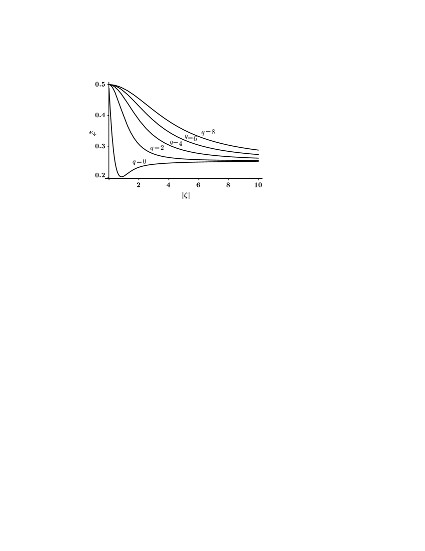
FIG. 1.: Plot of the least eigenvalue of the variance matrix for the pair coherent states as a function of $|zeta|\/$ for different values of $q\/$, demonstrating the $U(2)\/$ squeezing for these states.

A closer look at the rotation matrices $R_{1}(\theta)\/$ and $R_{2}(\theta)\/$ reveals that while $R_{2}(\theta)\/\in O(4)\cap Sp(4,R)\/$, the matrix $R_{1}(\theta)\/$ is an $O(4)\/$ transformation not in $Sp(4,R)\/$ because it cannot be written in the $S(X,Y)\/$ form. Thus the diaganalisation of the variance matrix $V(\zeta,q)\/$ is not possible within $U(2)\/$. The analysis in the preceding section shows that even though we are not able to diagonalise the variance matrix using compact canonical transformations we are fortunately able to bring the least eigenvalue to the leading diagonal position using such transformations. Physically this means that a new set of quadratures can be arrived at through some $S(X,Y)\/,\,\,U=X-iY\in U(2)\/$ such that one of them has its second noise moment equal to the least eigenvalue $e_{\downarrow}\/$ of the variance matrix $V(\zeta,q)$. To demonstrate this explicitly, consider a specific $U_{\psi}\in U(2)\/$ and the corresponding transformation $S(X,Y)\/$:

$$U_{\psi}=X_{\psi}-iY_{\psi}=\frac{1}{\sqrt{2}}\left[\begin{array}[]{cc}e^{-i\psi/2}&e^{-i\psi/2}\\ e^{i\psi/2}&-e^{i\psi/2}\end{array}\right]$$ (48)

$$X_{\psi}=\frac{1}{\sqrt{2}}\left[\begin{array}[]{cc}\cos{\frac{\psi}{2}}&\cos{\frac{\psi}{2}}\\ cos{\frac{\psi}{2}}&-\cos{\frac{\psi}{2}}\end{array}\right]$$ (51)

$$Y_{\psi}=\frac{1}{\sqrt{2}}\left[\begin{array}[]{cc}+\sin{\frac{\psi}{2}}&+\sin{\frac{\psi}{2}}\\ -\sin{\frac{\psi}{2}}&\sin{\frac{\psi}{2}}\end{array}\right]$$ (54)

$$S(X_{\psi},Y_{\psi})=\frac{1}{\sqrt{2}}\left[\begin{array}[]{rr}X_{\psi}&Y_{\psi}\\ -Y_{\psi}&X_{\psi}\end{array}\right].$$ (57)

Using the matrix $S(X_{\psi},Y_{\psi})\/$ we can obtained the transformed variance matrix

$$V^{\prime}(\zeta,q)=S(X_{\psi},Y_{\psi})V(\zeta,q)S(X_{\psi},Y_{\psi})^{T}$$ (58)

For a particular choice of $U_{\psi}\/$ with $\psi\/$ chosen to be the phase of $\zeta\/$, the transformed matrix $V^{\prime}(\zeta,q)\/$ has its least eigenvalue in the leading diagonal position. Therefore, for this particular value of $\psi\/$ the compact transformation $U_{\psi}\/$ gives us the new set of quadratures with one of them being the most squeezed one.

IV concluding Remarks

In this paper we have given a $U(2)\/$ invariant description of squeezing properties of the pair coherent states. For the pair coherent states the variance matrix is not diagonalisable through transformations within $U(2)\/$ and we have to use the full $O(4)\/$ for its diagonalisation. Therefore, these states provide an interesting example where the results of equation (25) has to be really used. We locate the least eigenvalue of the variance matrix $V(\zeta,q)\/$ by its explicit analytical diagonalisation through an $O(4)\/$ transformation which is outside $U(2)=O(4)\cap Sp(4,R)\/$, but the results of equations (24) and (25) ensure that we can also bring this smallest eigenvalue to the leading position (without diagonalising the variance matrix) by a suitable $U(2)\/$ transformation. We have constructed such a $U(2)\/$ transformation explicitly. This demonstrates the power and elegance of the group theoretic approach.

The smallest eigenvalue of the variance matrix $V(\zeta,q)\/$ turns out to be independent of the phase of $\zeta\/$, while the explicit $U(2)\/$ transformation which brings the least eigenvalue to the leading position depends upon the phase of $\zeta\/$. This shows that as we scan through states with different values for the phase of $\zeta\/$ we have to use different $U(2)\/$ transformations to locate the maximally squeezed quadrature. In fact the quadrature which is maximally squeezed is different for the states related to each other by such a phase factor.

In the usual analysis of squeezing one restricts oneself to a particular quadrature or a set of quadratures related to each other by certain subclass within $U(2)\/$. Normally this subclass is dictated by the measurement scheme being used. For the two-mode case for example, the usual analysis considers the subclass which can be explored through the heterodyne detection scheme. It is interesting to note that for the pair coherent states it indeed suffices to consider the heterodyne subclass and the set of transformations given in equation (57) are exactly those which can be explored using the heterodyne detection scheme [1]. This is in general not true and we must consider the group $U(2)\/$ in its entirety as a means to explore all the allowed quadratures for the two-mode fields.

Acknowledgement: The author thanks N. Mukunda and R. Simon for useful discussions.

REFERENCES

- [1] G.S. Agarwal, Phys. Rev. Lett. 57, 827 (1986).
- [2] G. S. Agarwal, J. Opt. Soc. Am. 5, 1940 (1988).
- [3] D. Bhaumik, K. Bhaumick, and B. Dutta-Roy, J. Phys. A 9 1507 (1976).
- [4] K. Tara and G. S. Agarwal, Phys. Rev. A 50, 2870 (1994).
- [5] A. Gilchrist, P. Deuar, and M. Reid, Phys. Rev. Lett. 80, 3169 (1998).
- [6] A. Gilchrist, P. Deuar, and M. Reid, Phys. Rev. A. 60, 4259 (1999).
- [7] W. Munro, Phys. Rev. A 59, 4197 (1999).
- [8] W. Munro, J. Opt. B, 2 47 (2000).
- [9] D. F. Walls, Nature, 280, 451 (1979).
- [10] D. F. Walls, Nature, 306, 141 (1983).
- [11] M. C. Teich and B. E. A. Saleh, Progress in Optics, 26, (1988).
- [12] J. R. Klauder and E. C. G. Sudarshan, Fundamentals of Quantum Optics, Benjamin, New York, (1968).
- [13] Arvind, Biswadeb Dutta, N. Mukunda and R. Simon, Phys. Rev. A52 1609 (1995).
- [14] Arvind and N. Mukunda, Phys. Lett. A 259 421-426 (1999).
- [15] R. Simon, N. Mukunda and B. Dutta, Phys. Rev. A 49, 1567 (1994).
- [16] B. Yurke, S. L. MacCall, and J. R. Klauder, Phys. Rev. A 33, 4033 (1986).
- [17] R. Simon and N. Mukunda Phys. Lett. A 143, 165 (1990).