Flow equation approach to diagonal representation of
an unbounded Hamiltonian with complex eigenvalues

Abstract

The flow equation approach investigated by Wegner et al. [1, 2, 3, 4] is applied to an unbounded Hamiltonian system with a generalization. We show that a well-known quantized complex energy eigenvalues which is related to decay widths can be given with this approach.

To investigate a quantum system, a diagonalization of a given Hamiltonian is one of mighty approaches. Eigenvalues and eigenstates which can be obtained with the diagonalized representation are most important clues to understanding of the physical properties of the system. But unfortunately, however there are a few explicitly solved exceptions, an analytically diagonalization of a given Hamiltonian is hard problem and various schemes have been deviced. Among of them, a novel approach to this problem was proposed by Wegner [1]. A way to construct of a generator, which generates one parameter unitary group which drives a given initial Hamiltonian to diagonalized (or almost diagonalized) final one, was deviced. This approach is called flow equation approach and it has already been applied to various physical models, especially condensed matter physics and high energy physics with some techniqal improvements[2, 3, 4].

On the other hand, there is interesting argument on the diagonalization, which is the diagonal representation of a Hamiltonian unbounded from below with complex eigenvalues. The imaginary part of the eigenvalues is related to the life-time of the quasi-stationary state, and it plays a good role to investigate a resonance phenomena[5, 6, 7, 8, 9, 10], however the eigenfunctions belonging to the complex eigenvalues can not be interpreted in a conventional sense. A mathematical treatment of the quasi-stationary approach has been also studied with a rigged Hilbert space (or Gel’fand triplet) formulation of quantum mechanics [8, 9, 10]. As pointed out by Bohm etal [8], such formulation allows for the description of the intrinsic irreversible processes in quantum mechanics, and these studies would be important in order to understand the fundamental relation between macroscopic irreversible phenomena and microscopic reversible theory.

Our interest is an investigation or generalization of Wegner’s flow equation to the unbounded system problems. In this letter, we consider one-dimensional quadratic interaction model (1), which becomes unbounded below in cases of $|\lambda_{0}/\omega_{0}|>1/2$. We show that the flow equation approach can be generalized to such situation where the original approach does not work, and this treatment provides a good scheme to study such deep features as a time arrow in quantum mechanics which were discussed in [8, 9, 10].

We shall consider a quadratic interaction system with the following Hamiltonian

$$H=\omega_{0}~{}a^{\dagger}a+\lambda_{0}~{}\left({a^{\dagger}}^{2}+a^{2}\right)+v_{0}$$ (1)

where $\omega_{0}$, $\lambda_{0}$ and $v_{0}$ are given constant of real numbers.

In order to explain the wegner’s approach and our interest, first, let us apply the original flow equation approach to this Hamiltonian (1). The flow equation is a continuous unitary transformation of the Hamiltonian, which is written in the following differential form;

$$\frac{dH(l)}{dl}=[\eta(l),H(l)],\quad\eta(l)=[H_{d}(l),H(l)]$$ (3)

or

$$H(l)=U^{\dagger}(l)H(0)U(l),\quad\frac{d}{dl}U^{\dagger}(l)=\eta(l)U^{\dagger}(l)$$ (4)

with the initial condition $H(0)=H$ (original (given) Hamiltonian). $H_{d}(l)$ is the diagonal portion of $H(l)$. Applying to the Hamiltonian (1), we obtain the following set of differential equations by coefficient matching:

$$\frac{d\omega(l)}{dl} = -16\omega(l)~{}\lambda(l)^{2}$$ (6)

$$\frac{d\lambda(l)}{dl} = -4~{}\omega(l)^{2}\lambda(l)$$ (7)

$$\frac{dv(l)}{dl} = -8~{}\omega(l)~{}\lambda(l)^{2},$$ (8)

where

$$H(l) = \omega_{0}a^{\dagger}(l)a(l)+\lambda_{0}~{}\left({a^{\dagger}(l)}^{2}+{a(l)}^{2}\right)$$ (10)

$$= \omega(l)a^{\dagger}a+\lambda(l)\left({a^{\dagger}}^{2}+a^{2}\right)+v(l)$$ (11)

$$H_{d}(l)=\omega(l)a^{\dagger}a+v(l),$$ (12)

and

$$a^{\dagger}(l)=U^{\dagger}(l)a^{\dagger}U(l),\quad a(l)=U^{\dagger}(l)aU(l)$$ (13)

with $~{}\omega(0)=\omega_{0},~{}\lambda(0)=\lambda_{0},~{}v(0)=v_{0}$. One can easily find that the solution of these equations has satisfied

$$\omega(l)^{2}-(2~{}\lambda(l))^{2}=\omega_{0}^{2}-(2~{}\lambda_{0})^{2}=const.$$ (15)

$$v(l)=v_{0}+\frac{1}{2}\left(\omega(l)-\omega_{0}\right).$$ (16)

Notice that there are two different type solutions whose behaviors are qualitatively different from each other (Fig.1).

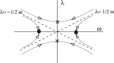
FIG. 1.: Schematical illustration of the unitary flow. The filled circles and crosses represent the fixed points (1) and (Flow equation approach to diagonal representation of an unbounded Hamiltonian with complex eigenvalues).

They can be distinguished by their initial points.

(i) $|\lambda_{0}/\omega_{0}|<1/2$ case

$$\omega(\infty) \rightarrow \omega_{0}\sqrt{1-4\left(\frac{\lambda_{0}}{\omega_{0}}\right)^{2}},$$ (18)

$$\lambda(\infty) \rightarrow 0,$$ (19)

$$v(\infty) \rightarrow v_{0}+\frac{1}{2}\left(\omega(\infty)-\omega_{0}\right),$$ (20)

(ii) $|\lambda_{0}/\omega_{0}|>1/2$ (unbounded) case

$$\omega(\infty) \rightarrow 0,$$ (22)

$$\lambda(\infty) \rightarrow \lambda_{0}\sqrt{1-\frac{1}{4}\left(\frac{\omega_{0}}{\lambda_{0}}\right)^{2}},$$ (23)

$$v(\infty) \rightarrow v_{0}-\frac{1}{2}\omega_{0}.$$ (24)

Notice that the diagonal representation ($\lambda(\infty)=0$) is obtained in the case of (i) ($|\lambda_{0}/\omega_{0}|<1/2$). This diagonal representation (1) can be understood in terms of famous Bogoliubov transformation, i.e.

$$H=\Omega b^{\dagger}b+\kappa+v_{0},\quad[b,b^{\dagger}]=1$$ (26)

where

$$\Omega=\frac{\omega_{0}}{\sinh^{2}\theta+\cosh^{2}\theta},\quad\kappa=-\frac{\omega_{0}\sinh^{2}\theta}{\sinh^{2}\theta+\cosh^{2}\theta}.$$ (27)

and

$$a=b\cosh\theta-b^{\dagger}\sinh\theta,\quad a^{\dagger}=b^{\dagger}\cosh\theta-b\sinh\theta,$$ (29)

with $\theta$ which satisfies

$$\frac{\lambda_{0}}{\omega_{0}}=\frac{\sinh\theta\cosh\theta}{\sinh^{2}\theta+\cosh^{2}\theta}.$$ (30)

One can easily check that relations (1) are completely equivalent to (1), i.e.,

$$\omega(\infty)=\Omega,\quad v(\infty)=\kappa+v_{0}.$$ (31)

The eigenvalues of (1) can be easily obtained from (1), that is

$$E_{n}=\Omega~{}n+\kappa+v_{0}\quad(n~{}\mbox{is integer}).$$ (32)

As it should be, the original flow equation approach works in this case (i).

In not only this case but also general cases where we can obtain a diagonal representation of a given Hamiltonian with this approach, the flow equation approach or the unitary transformation $U(\infty)$ can be interpretated as a transformation of the basis from one which diagonalizes $H_{d}(0)$ to another which diagonalize $H(0)$. We can say this original approach works when both of the basis are in a same function space because $U(\infty)$ is unitary. On the other hand, in the case of (ii) it is clear that the eigenstates of the Hamiltonian is only scattering states and they can not be in a same function space with eigenstates of $H_{d}(0)$ (boundary state). Therefore it is rather reasonable that the original approach does not work, as we saw in (Flow equation approach to diagonal representation of an unbounded Hamiltonian with complex eigenvalues).

It would be obvious that some generalization to larger class flow should be required to obtain the diagonal representation of the Hamiltonian. The key should be to remove the unitarity from the flow equation approach and that it can be realized in the following procedure.

Generally, flows with the differential equation of the first-order like equation (4) does not have any crossing points with each other, except for the attractor points. Thus we would expect that some different flows whose attractor points are common will be related to each other. A diagonal representation of an unbounded Hamiltonian is also obtained with some new flow which has same attractor points with the original (unitary) one, however this new flow would not represent an unitary transformation, unlike the original flow. General solutions of Eq.(4) which has a attractor point (Flow equation approach to diagonal representation of an unbounded Hamiltonian with complex eigenvalues) can be written as

$$\omega(l) = 2\lambda(\infty)\left(\cos\varphi_{l}\sinh\xi_{l}+i\sin\varphi_{l}\cosh\xi_{l}\right),$$ (34)

$$\lambda(l) = ~{}\lambda(\infty)~{}\left(\cos\varphi_{l}\cosh\xi_{l}+i\sin\varphi_{l}\sinh\xi_{l}\right),$$ (35)

$$v(l) = v_{0}+\frac{1}{2}\left(\omega(l)-\omega_{0}\right),$$ (36)

where

$$\frac{d}{dl}\xi_{l} = -8\lambda(\infty)\cos 2\varphi_{l}\sinh 2\xi_{l},$$ (38)

$$\frac{d}{dl}\varphi_{l} = -8\lambda(\infty)\sin 2\varphi_{l}\cosh 2\xi_{l}$$ (39)

with

$$\xi_{\infty}\rightarrow 0,\quad\varphi_{\infty}\rightarrow 0.$$ (40)

It should be noticed that the real (unitary) flow is one of the solutions represented with (1), i.e., $\varphi_{l}=0$, and there are two other separable solutions i.e., $\varphi_{l}>0$ ($\varphi_{l}\rightarrow+0$ as $l\rightarrow\infty$) and $\varphi_{l}<0$ ($\varphi_{l}\rightarrow-0$ as $l\rightarrow\infty$). which are originated from unstable fixed-points

$$(\omega,\lambda)=(\pm 2i\lambda(\infty),0),~{}\left(\mbox{or}~{}(\xi,\varphi)=(0,\pm\frac{\pi}{2})\right).$$ (41)

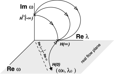
FIG. 2.: Schematical illustration of the generalized flows $H^{(0)}(l)$ and $H^{(+)}(l)$.

There are three kinds of flows which have a common attractor point $\left(0,\lambda(\infty)\right)$ but different “initial ($l\rightarrow-\infty$)” points, $\left(2i\lambda(\infty),0\right)$, $\left(-2i\lambda(\infty),0\right)$, and “somewhere on the real flow plane”. Corresponding to them, we can introduce three Hamiltonian-flows, i.e., $H^{(\pm)}(l)$ and $H^{(0)}(l)$ as

$$H^{(j)}(l) = \omega^{(j)}(l)a^{\dagger}a+\lambda^{(j)}(l)\left({a^{\dagger}}^{2}+a^{2}\right)+v^{(j)}(l)$$ (42)

$$(j = \{\pm,0\}),$$ (43)

with

$$\omega^{(\pm)}(- \infty)\rightarrow\pm 2i\lambda(\infty),~{}\lambda^{(\pm)}(-\infty)\rightarrow 0,$$ (46)

$$\left(v^{(\pm)}(-\infty)\rightarrow v(\infty)\pm i\lambda(\infty)\right)$$

and

$$\omega^{(0)}( 0)=\omega_{0},~{}\lambda^{(0)}(0)=\lambda{{}_{0}},~{}\left(v^{(0)}(0)=v_{0}\right).$$ (47)

It is obvious that these Hamiltonian-flows are attracted to the common fixed point (Flow equation approach to diagonal representation of an unbounded Hamiltonian with complex eigenvalues) as $l\rightarrow\infty$, i.e.,

$$\omega^{(j)}(\infty)\rightarrow 0,~{}\lambda^{(j)}(\infty)\rightarrow\lambda(\infty),~{}v^{(j)}(\infty)\rightarrow v(\infty).$$ (48)

Precisely speaking, (Flow equation approach to diagonal representation of an unbounded Hamiltonian with complex eigenvalues) and (Flow equation approach to diagonal representation of an unbounded Hamiltonian with complex eigenvalues) are not sufficient to define $H^{(\pm)}(l)$ uniquely. They depend on direction of an “infinitesimal shift” from the fixed points. Giving this direction is giving some complex number $\varphi_{\infty}/\xi_{\infty}$. For example, $\varphi_{\infty}/\xi_{\infty}=0$ corresponds to $H^{(0)}(l)$.

The Hamiltonian flow $H^{(0)}(l)$ is the unitary flow described in (Flow equation approach to diagonal representation of an unbounded Hamiltonian with complex eigenvalues), and that not $H^{(0)}(l)$ but $H^{(\pm)}(l)$ give us the diagonal representation of the original Hamiltonian (1) with complex eigenvalues (at $l\rightarrow-\infty$), i.e.

$$H^{(\pm)} (-\infty)=\pm 2i\lambda(\infty)~{}a^{\dagger}a+v^{(\pm)}(-\infty)$$ (51)

$$=\pm 2i\lambda_{0}\sqrt{1-\frac{1}{4}\left(\frac{\omega_{0}}{\lambda_{0}}\right)^{2}}~{}\left(a^{\dagger}a+\frac{1}{2}\right)+v(\infty)$$

$$\equiv\pm i\gamma~{}\left(a^{\dagger}a+\frac{1}{2}\right)+v(\infty).$$

We can immediately obtain the quantized complex eigenvalues

$$E^{(\pm)}_{n}=\pm i{\gamma}\left(n+\frac{1}{2}\right)+v(\infty)\quad(n~{}\mbox{is integer}),$$ (52)

and this is consistent with well-known result (for example, see [9, 10]). The symmetry in (52) is related to symmetric phenomena in unstable system, that is, “decaying process for the positive time” and “growing process for the negative time”, as was pointed out in [5, 6, 7, 8, 9, 10]. On should notice that the infinitesimal shift from the attractor point (Flow equation approach to diagonal representation of an unbounded Hamiltonian with complex eigenvalues) decides the arrow of time of the phenomena. This means that the structure of the generalized flow should be directly connected to the deep features of an irreversible process which described with quantum mechanics.

Let us mention to applications of our approach to other models.

First, this approach seems possible to apply easily to other models, however we have to be careful of the following fact. In general, when our approach is applied to some systems, a truncation schemes to get a closed set of differential equations would be often required, since the higher interactions will be generated with the “evolution” $U(l)$. In such cases, we can adopt some truncation schemes which have already been proposed for the ordinary flow equation approach [3, 4] in which we can consider non-perturbative corrections.

Second, in general cases it is almost impossible to solve the set of equations analytically because they becomes highly nonlinear even after the trancation. Therefore, sometimes, we have to study generalized flow equations numerically. In the numerical studies, the following procedure to find an unstable fixed point (which gives a diagonal representation of unbounded Hamiltonian) would be useful.

1. Find a stable fixed point (like (Flow equation approach to diagonal representation of an unbounded Hamiltonian with complex eigenvalues)) with the forward ($l\rightarrow\infty$) evolution with the unitary flow from original (given) Hamiltonian. This process should be always easy because the point is a attractor point.

2. After finding the fixed point, compute the backward evolution from the “initial” point which is slightly (infinitesimally) shifted to some direction from the attractor point.

The flow will be “attracted” to the unstable point as $l\rightarrow-\infty$, and we should easily find the unstable fixed points as “attractors”. There must be such symmetric two unstable points which depend on the direction of the “initial” infinitesimal shift. (This corresponds to two Hamiltonian flows $H^{(\pm)}(l)$ for (1). )

Finally, let us mention to an application of our approach to a so-called open system problems. As well known, there are two kinds of discussion about the time arrow in quantum mechanics [8]. One is called the intrinsic irreversibility and the other is called the extrinsic irreversibility. The decaying process of state with the Hamiltonian (1) is thought as an example of the former, and the decay with an interaction with environment is thought as the latter or as a dynamics of the open system [11, 12]. Dealing with the open system is another standard approach to introduce the time arrow to quantum mechanics. It should be interesting problem to apply our approach to open systems. Actually spin-boson model which is a typical model to discuss the extrinsic decaying process [12], was studied within an (improved but) unitary flow equation approach by Mielke etal [4], and they succeeded in computing the energy shift of spin system which is due to the interaction with the bosonic environment. But decay constants was not obtained directly and the dissipative property of the system seems hard to be understood from their analysis. We think our approach can be used to reexamine this system and the dissipative properties of this system can be made clearest. Moreover it will be helpful to understand the relation between two different treatment on the irreversibility in quantum mechanics.

Kentaro Imafuku is grateful to Centro Vito Volterra and Luigi Accardi for kind hospitality. He is supported by a overseas research fellowship of Japan Science and Technology Corporation.

REFERENCES

- [1] F. Wegner, Ann. Phys. (Leipzig) 3 (1994) 77.
- [2] P. Lenz, and F. Wegner, Nucl. Phys. B482 (1996) 693.
- [3] S. K. Kehrein, and A. Mielke, Phys. Lett. A 219 (1996) 313; Ann. Phys. (Leipzig) 6, (1997) 90; A. Mielke, Ann. Phys. (Leipzig) 6 (1997) 215; Europhys. Lett. 40 (1997) 195-200.
- [4] Stefan K. Kehrein, Andreas Mielke, and Peter Neu, Z. Phys B 99 (1996) 269-280; A. Mielke, Eur. Phys. J. B5 (1998) 605-611;
- [5] G. Gamov, Z. Physik 51 (1928) 204
- [6] N. Nakanishi, Prog. Theor. Phys. 19 (1958) 607
- [7] J. Aguilar and J. M. Combes, Commun. Math. Phys.22 (1971) 269; E. Balslev and J. M. Combes, ibid p.p.280
- [8] A. Bohm, S. Maxon, Mark Loewe, M. Gadella, Physica A 236 (1997) 485-549; A. Bhom and M. Gadella, Dirack Kets, Gamov Vectors and Gel’fand Triplets (Lecture Notes in Physics, Vol. 348, Sprnger, 1989)
- [9] T. Shinbori, and T. Kobayasi, Nuovo Cim. B 115 (2000) 325;
- [10] T. Shinbori, Phys. Lett. A 273 (2000) 37-41
- [11] R. P. Feynman and F. L. Vernon, Ann. Phys. 24, 118 (1963); R. P. Feynman and A. R. Hibbs, Quantum Mechanics and Path Integrals (McGraw-Hill, New York, 1965), A. O. Caldeira and A. J. Leggett, Ann. Phys. 149, 374 (1983); 153, 445(E) (1984); Physica 121A, 587 (1983); 130A, 374(E) (1985)
-
[12]
A. J. Leggett, S. Chakravarty, A. T. Dorsey, M. P. A.
Fisher, A. Garg, and W. Zwerger, Rev. Mod. Phys. 59, 1 (1987).