Phase transitions in a one-dimensional multibarrier potential of finite range

D.Bar^a and L.P.Horwitz^a,b

^aDepartment of Physics, Bar Ilan University, Ramat Gan, Israel
^bRaymond and Beverly Sackler Faculty of Exact Science, School of Physics, Tel Aviv University, Ramat Aviv, Israel

Abstract

We have previously studied properties of a one-dimensional potential with $N$ equally spaced identical barriers in a (fixed) finite interval for both finite and infinite $N$. It was observed that scattering and spectral properties depend sensitively on the ratio $c$ of spacing to width of the barriers (even in the limit $N\to\infty$). We compute here the specific heat of an ensemble of such systems and show that there is critical dependence on this parameter, as well as on the temperature, strongly suggestive of phase transitions.

PACS number(s): 05.70.Fh, 02.60.Cb, 03.65.Ge

1 Introduction

We have studied the one-dimensional locally periodic multibarrier potential of finite range for both finite and infinite number $N$ of barriers. We found [1] that there is a critical dependence of the transmission coefficient, the cross section and the distribution of poles of the $S$-matrix [2] on the ratio $c$ of the total interval between the barriers to their total width. Under certain conditions this model was found to contain signatures of chaotic behaviour [3], such as rapid spread of wave packets and Wigner type spectral characteristics.

We discuss in this work thermodynamic properties [4] such as the specific heat and the entropy of an ensemble of such systems and show that they also depend critically upon this ratio in addition to their dependence upon the temperature. We show that when the number of barriers is not large there are no low-lying energy eigenvalues for small values of the ratio $c$. These values of $c$ depend upon the value of the number $N$ of barriers in such a manner that the ranges of $c$ in which this part of the energy spectrum is missing increase at first with $N$ and then decrease as $N$ continue to grow until they disappear entirely for large enough $N$. Above the upper boundaries of these ranges are the points where the energy spectrum contains eigenvalue distribution over all energies. A similar phenomenon occurs in the work of Fendley and Tchernyshyov [5] on one-dimensional phase transitions, where the seriously disordered phase behaves as if it were at very high temperature, where the effect of interactions is relatively small, i.e, as an almost independent particle model. This apparently accounts, even for neighbouring values of $c$ within these ranges, for large changes in the average energy and all the other statistical mechanics properties, such as specific heat and entropy, derived from it. For example, the corresponding curves of the specific heat, for these neighbouring values of $c$, as functions of the temperature, differ markedly from each other, as will be shown in the following, when plotting these curves in a single figure. This sensitivity of the specific heat is largest for intermediate values of $N$ and $c$ in which the curves of the specific heats as functions of the temperature differ to the extent that some of them exhibit double peak phase transitions while other curves, for neighbouring values of $c$, resemble the conventional Debye curve [4] which characterizes the solid crystal. For infinite $N$, as will be shown, the double peak phase phenomenon is retained even for large values of $c$. Also, we find, for all values of $N$ and $c$, indication of phase transitions in specific heat at small values of the temperature $T$. We note that for any $c$, which is greater than some value which depends upon $N$, the system behaves for all $N$, except for a spike form at small $T$, in a manner similar to that of the solid crystals in which the constituent atoms are widely separated, and thus, as we have remarked, are characterized by large values of the ratio $c$. This is seen on the corresponding graphs of the specific heats as functions of the temperature which have the same form as that of Debye (we do not imply here that our system is analogous to a system of lattice vibrations, but only to the behaviour of the result due to the apparent presence of uncorrelated modes).

In Section 2 we study the properties of a one-dimensional $N$ potential barrier system when $N$ is a finite number. In Section 3 we discuss the limit of $N\to\infty$ (in the same fixed interval). For both cases we find abrupt and large changes in the values of specific heat and entropy for small values of the temperature $T$. These large changes suggest the existence of phase transitions. In particular, for intermediate $N$ and $c$, we find double peaks [6, 7, 8, 9] in the specific heat curves. Double peak phase transitions appear, especially, for infinite $N$ in which it remains effective even for large values of $c$. Tanaka et al [7] have found double peak structures in anti-ferromagnetic materials, corresponding to magnetic phases, where the external magnetic field seems to play a role somewhat analogous to the parameter $c$ in our study. Leung and Neda [6] and also Kim et al [8] have found double peaks in the response curves, apparently associated with dynamically induced phase transitions. Ko and Asakawa [9] have also found a double peak structure in their calculations of the phases of a quark-gluon plasma, where one may think of a large number of interactions in a bounded region. We do not imply that our model contains an analog of their interacting systems, but suggest that some of the mathematical properties may be common.

2 The one-dimensional $N$ potential barrier system

We consider a finite $N$ barrier system where all these barriers have the same height $v$ and are locally periodic in the finite interval. This array is assumed to start at the point $x=-\frac{a+b}{2}$ and ends at $x=\frac{a+b}{2}$, so that the total length of this system is $L=a+b$. Here $a$ is the total width of all the $N$ barriers (where $v\neq 0$), and $b$ is the total sum of all the intervals between neighbouring barriers (where $v=0$). Thus, since we have $N$ potential barriers the width of each one is $\frac{a}{N}$, and the interval between each two neighbouring ones is $\frac{b}{N-1}$. Denoting $b=ac$ where $c$ is a real number we can express $a$ and $b$ in terms of $L$ and $c$ as [1] $a=\frac{L}{1+c},\;\;\;\;\;b=\frac{Lc}{1+c}$.

Let us first consider the passage of a plane wave through this system, which has the form $\phi=A_{1}e^{ikx}+B_{1}e^{-ikx},\ \ \ x\leq-\frac{a+b}{2}$. Matching boundary conditions at the beginning and end of each barrier, we may construct a solution in terms of the transfer matrices [2, 11] $P^{(j)}$ on the $j$th barrier. After the $n$th barrier we obtain, using the terminology in [2], the following transfer equation [1]

$$\left[\begin{array}[]{c}A_{2n+1}\\ B_{2n+1}\end{array}\right]=P^{(n)}P^{(n-1)}\ldots P^{(2)}P^{(1)}\left[\begin{array}[]{c}A_{1}\\ B_{1}\end{array}\right],$$ (1)

where $p^{(n)}$ is a product of three two dimensional matrices [1]. $A_{2n+1}$ and $B_{2n+1}$ are the amplitudes of the transmitted and reflected parts respectively of the wave function at the $n$th potential barrier. $A_{1}$ is the coefficient of the initial wave that approaches the potential barrier system, and $B_{1}$ is the coefficient of the reflected wave from the first barrier. Eq (1) may be written as [1]

$$\left[\begin{array}[]{c}A_{2n+1}\\ B_{2n+1}\end{array}\right]=\left[\begin{array}[]{c c}e^{-ik(a+b-\frac{a}{2N})}&0\\ 0&e^{ik(a+b-\frac{a}{2N})}\end{array}\right]\left[\begin{array}[]{c c}T_{11}&T_{12}\\ T_{21}&T_{22}\end{array}\right]\Biggl{(}\left[\begin{array}[]{c c}e^{\frac{ikb}{N-1}}&0\\ 0&e^{-\frac{ikb}{N-1}}\end{array}\right]\left[\begin{array}[]{c c}T_{11}&T_{12}\\ T_{21}&T_{22}\end{array}\right]\Biggr{)}^{n-1}\cdot$$ (12)

$$\cdot\left[\begin{array}[]{c c}e^{\frac{-ika}{2N}}&0\\ 0&e^{\frac{ika}{2N}}\end{array}\right]\left[\begin{array}[]{c}A_{1}\\ B_{1}\end{array}\right]=Q\left[\begin{array}[]{c}A_{1}\\ B_{1}\end{array}\right],$$ (19)

where $k$ is $\sqrt{\frac{2me}{\hbar^{2}}}$. Note that the transfer equation (19) is valid for both cases of $e>v$ and $v>e$ except for the two-dimensional matrix in $T$ which, for the $e>v$ case, assumes the form

$$T_{11}=\cos(\frac{aq}{N})+i\frac{\xi}{2}\sin(\frac{aq}{N}),\;\;\;T_{12}=i\frac{\eta}{2}\sin(\frac{aq}{N})$$ (20)

$$T_{21}=-i\frac{\eta}{2}\sin(\frac{aq}{N}),\;\;\;T_{22}=\cos(\frac{aq}{N})-i\frac{\xi}{2}\sin(\frac{aq}{N}),$$

and for the $v>e$ case

$$T_{11}=\cosh(\frac{aq}{N})+\frac{\grave{\xi}}{2}\sinh(\frac{aq}{N}),\;\;\;T_{12}=\frac{\grave{\eta}}{2}\sinh(\frac{aq}{N})$$ (21)

$$T_{21}=-\frac{\grave{\eta}}{2}\sinh(\frac{aq}{N}),\;\;\;T_{22}=\cosh(\frac{aq}{N})-\frac{\grave{\xi}}{2}\sinh(\frac{aq}{N})$$

The $q$, $\xi$ and $\eta$ of Eq (20) are [1] $q=\sqrt{\frac{2m(e-v)}{\hbar^{2}}},\ \ \ \ \xi=\frac{q}{k}+\frac{k}{q},\quad\eta=\frac{q}{k}-\frac{k}{q},$ and those of Eq (21) [1] $q=\sqrt{\frac{2m(v-e)}{\hbar^{2}}},\ \ \ \ \grave{\xi}=-i\eta=\frac{q}{ik}+\frac{ik}{q},\quad\grave{\eta}=-i\xi=\frac{q}{ik}-\frac{ik}{q}$. In the numerical part of this work we assign $\hbar=1$, and $m=\frac{1}{2}$. Note that the two matrices $T$ from Eqs (20)-(21) do not depent on $n$.

We find, now, the energy spectrum of this system. We use the $S$-matrix and the periodic boundary conditions at the two remotely placed sides of the system. That is, we assume that the wave function and its derivative at the far right end of the system, say at $x=C$ where $C$ is much larger than the size $L=a+b$ of the system, are equal to the wave function and its derivative at the corresponding far left end of the system at $x=-C$, so we obtain $A_{2N+1}e^{ikC}=A_{1}e^{-ikC}$, $B_{2N+1}e^{-ikC}=B_{1}e^{ikC}$. Thus, using the last relation and those between the components of the $S$ and $Q$ matrices [2], where $Q$ is given by Eq (19),

$$S_{11}=Q_{11}-\frac{Q_{12}Q_{21}}{Q_{22}}=\frac{1}{Q_{22}},\;\;\;\;S_{12}=\frac{Q_{12}}{Q_{22}},\;\;\;\;S_{21}=-\frac{Q_{21}}{Q_{22}},\;\;\;\;S_{22}=\frac{1}{Q_{22}},$$

one may write the following dependence of the outgoing waves $A_{2N+1}$ and $B_{1}$ upon the ingoing ones $A_{1}$ and $B_{2N+1}$

$$\left[\begin{array}[]{c}A_{2N+1}\\ B_{1}\end{array}\right]=\left[\begin{array}[]{c c}S_{11}&S_{12}\\ S_{21}&S_{22}\end{array}\right]\left[\begin{array}[]{c}A_{1}\\ B_{2N+1}\end{array}\right]=e^{2ikC}\left[\begin{array}[]{c c}S_{11}&S_{12}\\ S_{21}&S_{22}\end{array}\right]\left[\begin{array}[]{c}A_{2N+1}\\ B_{1}\end{array}\right]=$$ (32)

$$=\frac{e^{2ikC}}{Q_{22}}\left[\begin{array}[]{c c}1&Q_{12}\\ -Q_{21}&1\end{array}\right]\left[\begin{array}[]{c}A_{2N+1}\\ B_{1}\end{array}\right]$$ (37)

To obtain a non trivial solution for the vector $\left[\begin{array}[]{c}A_{2N+1}\\ B_{1}\end{array}\right]$ one must solve the following equation

$$\det\left[\begin{array}[]{c c}\frac{e^{2ikC}}{Q_{22}}-1&\frac{e^{2ikC}Q_{12}}{Q_{22}}\\ -\frac{e^{2ikC}Q_{21}}{Q_{22}}&\frac{e^{2ikC}}{Q_{22}}-1\end{array}\right]=\frac{\cos(4kC)}{Q_{22}^{2}}-\frac{2\cos(2kC)}{Q_{22}}+1+$$ (40)

$$+\frac{Q_{12}Q_{21}\cos(4kC)}{Q_{22}^{2}}+i(\frac{\sin(4kC)}{Q_{22}^{2}}-\frac{2\sin(2kC)}{Q_{22}}+\frac{Q_{12}Q_{21}\sin(4kC)}{Q_{22}^{2}})=0$$

The form of the equations (32)-(40) are the same for both cases of $e>v$ and $v>e$ except for the two-dimensional matrix $Q$ from Eq (19) in which the matrix $T$ assumes the form (20) for the $e>v$ case and the form (21) for $v>e$. The energies, satisfying this relation, depend, as noted, on $c$ and $N$ and are obtained numerically. We show, now, that the high energy part ($e>\!>v$) of the spectrum obtained from Eq (40) depends only on $C$ and may be obtained analytically without using numerical methods. For that matter we note that when the energy $e$ becomes very large we have $k\approx q$, and $\xi$ and $\eta$ (see the inline equations after Eq (21)) obtain the values of 2 and 0 respectively. In that case the components $T_{12}$ and $T_{21}$ of the two dimensional matrix $T$ from Eq (20) become zero, and the diagonal elements $T_{11}$ and $T_{22}$ become $e^{\frac{iqa}{N}}$ and $e^{-\frac{iqa}{N}}$ respectively. Thus, the two dimensional matrix $Q$ from Eq (19) becomes much simplified and may be calculated analytically as follows (using $q\approx k$ for the very high part of the energy spectrum)

$$Q_{(high-energies)}=\left[\begin{array}[]{c c}e^{-ik(a+b-\frac{a}{2N})}&0\\ 0&e^{ik(a+b-\frac{a}{2N})}\end{array}\right]\left[\begin{array}[]{c c}e^{\frac{ika}{N}}&0\\ 0&e^{-\frac{ika}{N}}\end{array}\right]\cdot$$ (45)

$$\cdot\Biggl{(}\left[\begin{array}[]{c c}e^{ik(\frac{b}{N-1}+\frac{a}{N})}&0\\ 0&e^{-ik(\frac{b}{N-1}+\frac{a}{N})}\end{array}\right]\Biggr{)}^{n-1}\left[\begin{array}[]{c c}e^{-\frac{ika}{2N}}&0\\ 0&e^{\frac{ika}{2N}}\end{array}\right]=$$ (50)

$$=\left[\begin{array}[]{c c}e^{-ik(a(1-\frac{3}{2N})+b-(n-1)(\frac{b}{N-1}+\frac{a}{N})+\frac{a}{2N})}&0\\ 0&e^{ik(a(1-\frac{3}{2N})+b-(n-1)(\frac{b}{N-1}+\frac{a}{N})+\frac{a}{2N})}\end{array}\right]=$$ (53)

$$=\left[\begin{array}[]{c c}e^{-ik(a+b+\frac{b}{N-1}-n(\frac{b}{N-1}+\frac{a}{N}))}&0\\ 0&e^{ik(a+b+\frac{b}{N-1}-n(\frac{b}{N-1}+\frac{a}{N}))}\end{array}\right]=\left[\begin{array}[]{c c}1&0\\ 0&1\end{array}\right],$$ (58)

for $n=N$, required for the application of (40). Thus we see that the two dimensional matrix $Q$ becomes the unity matrix in the limit of large energies $e$. Substituting the resulting components of $Q$ ($Q_{11}=Q_{22}=1$, $Q_{12}=Q_{21}=0$) in Eq (40) we obtain

$$\det\left[\begin{array}[]{c c}e^{2ikC}-1&0\\ 0&e^{2ikC}-1\end{array}\right]=(e^{2ikC}-1)^{2}=0$$ (59)

The last equation is satisfied for all $k=\frac{\pi n}{C},\;\;\;n=0,1,2,3\ldots$, but since we are restricted here to the high energy part of the energy spectrum we refer only to the large values of $n$.

As remarked, the previous equations may be applied also for the $e<v$ case except for the correct $Q$. Thus, the energy spectrum is composed of three parts: 1) the part for the $e<v$ case. 2) the part that satisfies $e_{n_{0}}>e>v$, where $e_{n_{0}}$ is some arbitrarily specified large energy (these two parts are obtained numerically by solving Eq (40) for both cases of $e>v$ and $e<v$ case with the appropriate $Q$), and 3) all the high energies that are larger than $e_{n_{0}}$ and are obtained analytically using Eqs (50), (59) and the relation $k=\frac{\pi n}{C}\;\;\;\;n=n_{0},n_{0}+1,n_{0}+2\ldots$, where $n_{0}$ is some specified large integer that corresponds to the energy $e_{n_{0}}$. Now, since the relation between the energy $e$ and $k$ is $k=\sqrt{e}$ (as remarked, we assign $\hbar=1$ and $m=\frac{1}{2}$), the high part of the energy spectrum is given by $e_{high}=(\frac{\pi n}{C})^{2}$, where $n=n_{0},n_{0}+1,n_{0}+2,\ldots$. For the numerical part of the calculations we assign the following values for the relevant parameters: $v=60$, $C=90$, $L=20$, and $e_{n_{0}}=1080$. Thus, the $e<v$ part of the spectrum is $0<e<60$. The second part is $60<e<1080$, and the third part is $e>1080$. The $n_{0}$ that corresponds to $e_{n_{0}}$ is $n_{0}=\frac{C}{\pi}\sqrt{e_{n_{0}}}\approx 941$. The assigned values for $C$ and $L$ yield a ratio of $\frac{C}{L}=4.5$ which ensures that the points $x=\pm C$ are far enough from the region of the potential and so we may assume (see the discussion after Eq (21)) that the values of the wave function and its derivative at $x=+C$ are equal to these at $x=-C$. These equalities are needed for obtaining Eqs (32)-(40). Thus, the results of the numerical simulations depend upon the ratio $\frac{C}{L}$ and not upon the specific values of $C$ and $L$. The somewhat higher value of the potential $v=60$ (the value, conventionally chosen for numerical simulations (see [13]), is from the range $(2\leq v\leq 8)$) is especially chosen for the $e<v$ part of the simulations in order to accumulate enough data and thus to obtain a better statistics. Note that the simulated $e_{n_{0}}>e>v$ part, where $e_{n_{0}}=1080$, yields a large amount of data so that in order not to remain with a comparatively small amount for the $e<v$ part we have chosen, as remarked, a somewhat large value of $v$. The value of $e_{n_{0}}=1080$ is chosen as a limit value beyond which the corresponding terms of the sums $\sum e(c,N)e^{-\beta e(c,N)}$ and $\sum e^{-\beta e(c,N)}$ in the following Eq (60) may be approximated by their simplified analogs obtained using Eq (59). Thus, the results are not sensitive to these specific values of $C$, $L$, $v$, and $e_{n_{0}}$.

We want to obtain a formula for the average energy from which we may derive most of the statistical mechanics parameters mentioned above. This average energy depends upon $c$, $C$, $N$ and the temperature $T$ (the dependence upon the temperature is through $\beta=\frac{1}{\kappa T}$, where $\kappa$ is the Boltzman constant which is assigned, in our numerical work, the value of unity) and is given by

$$<\!e\!>(\beta,c,N)=\frac{\sum e(c,N)e^{-\beta e(c,N)}+\sum_{941}^{\infty}(\frac{n\pi}{C})^{2}e^{-\beta(\frac{\pi n}{C})^{2}}}{\sum e^{-\beta e(c,N)}+\sum_{941}^{\infty}e^{-\beta(\frac{\pi n}{C})^{2}}},$$ (60)

where the first sum in the numerator and denominator contains the contributions from all $e(c,N)<1080$. For higher values of $e$ the expressions are simpler and we take this into account in the second sum over all integers $941\leq n$. The first sum in the numerator and denominator of Eq (60) includes the energies from the $e<v$ and the $v<e<1080$ parts of the spectrum . These parts are obtained numerically from Eq (40) in which we substitute for the components of $Q$ from Eq (19), using the $T$’s of Eq (20) for the $e>v$ case, and those of Eq (21) for $e<v$. From Eq (60) we obtain an average energy for each specific triplet of values for $c$, $N$, and $\beta$, and from this average energy we may derive the quantities of statistical physics. We note that the sums over the energies from the range $0.1\leq e\leq 1080$ depend upon the parameters $N$ and $c$ whereas the sums over the higher energies do not depend upon them (see Eqs (50), (59)). The specific heat $C_{h}$ is obtained as the derivative of the average energy from Eq (60) with respect to the temperature $T$.

It is found that for large values of the temperature $T$ the curves of the specific heats $C_{h}$, for all values of $c$ and $N$, tend to the constant value $C_{h}=0.55$. That is, for these $T$’s the curves of $C_{h}$ become as expected a constant curve as for Dulong-Petit [4]. Also, for small $T$’s the curves of $C_{h}$, for all $c$ and $N$, rise rapidly to their maximum values $C_{h_{max}}$ from which they descend either to the asymptotic value of 0.55 for large $T$ as noted or to some minimum from which they rise again to a second peak that descends to the value of 0.55 for large $T$. We note that the $C_{h_{max}}$’s are points at which the derivative appears to be very large and are, therefore, suggestive of the existence of phase transition [10]. The values of these $C_{h_{max}}$, however, as well as the behavior of the specific heat for intermediate values of $T$ depend upon $c$ and $N$. It has been found that for large $c$ the curves of the specific heats, as functions of $T$, are of the Debye type [4], that is, the rapid approach to maximum $C_{h_{max}}$ for small $T$ and the immediate decrease to a constant value as $T$ grows. For small $c$, however, the forms of the specific heat $C_{h}$ for intermediate $T$ depart markedely from that of Debye, and the range of $T$ in which $C_{h}$ is different depends upon $N$ in such a manner that this range increases as $N$ grows. For example, when $N=2$ this range is $0.4\leq T\leq 3.8$, for $n=35$ it is $0.4\leq T\leq 100$ and for $N=250$ this range increases to $5\leq T\leq 2000$.

Figure 1 shows 38 curves of the specific heats, for $N=6$, as functions of the temperature in the range $0.1\leq T\leq 35$. Each curve is for a different integral value of $c$ in the range $2,3,\ldots,39$. The central and dense part of the figure, where a large part of the curves have the same form, are those graphs that have a large $c$ and, therefore, may represent the solid crystals that are characterized by a periodic structure in which neighbouring occupied sites are widely separated. Indeed, these curves resemble, except for the sharp peaks, that of Debye which represents well the solid crystal. The other curves that differ from the central ones, and that generally have large values for the specific heats at small $T$, are those that have smaller $c$ and, therefore, do not have the behaviour of the specific heat curves of a solid crystal. These curves may represent some "soft" substance [12] in which the constituent atoms or molecules are closer to one another than in the solid crystal. These substances have Einstein frequencies [4, 12] smaller than those of the solid crystals by a factor of 10 to 50 [12] and, therefore, are characterized by higher values of the specific heats. Also, the remarked sharp peaks have a very large value for the derivative and this suggests an existence of phase transitions. We have, especially, studied the immediate neighbourhood of the region containing rapid variation in specific heat as a function of temperature and the parameter $c$ (i.e, the neighbourhood of a phase transition). We see that there is a very strong and critical dependence on $c$. This result illustrates the physical mechanism for the formation of such rapid transitions, a resonance-like phenomena controlled by the geometry of the barrier system. This is demonstrated in Figure 2 which shows 15 curves of the specific heat, for $N=6$, as functions of the temperature $T$ and for the following values of $c=0.3,0.4,0.5,\ldots 1.7$. The central dense part of the figure, which is composed of 9 curves, is drawn for the larger values of $c$ whereas the remaining 6 curves are for the smaller $c$’s. Note that although the difference in $c$ for any two neighbouring curves is only 0.1 nevertheless the upper curves in the figure differ significantly in appearance from each other and from those of the central part.

Fendley and Tchernyshyov [5] have discussed one-dimensional phase transitions in systems with infinite number of degrees of freedom per site. They argue that a singularity of the maximum eigenvalue in the "transfer matrix" (their model considers a set of systems with SU(N) type symmetry) causes a phase transition. The $N\to\infty$ limit of [5] corresponding to an infinite number of degrees of freedom per site is replaced, in our case, by a large (infinite) number of barriers in a finite interval. The transfer matrix that we have introduced connecting neighbouring sites (barrier-gap structures) is independent of $\beta$ (inverse temperature), but the eigenvalue of the total transfer matrix of the infinite system has a branch point as we show in Section 3. This singularity can influence the behaviour of the partition function, resulting, as in [5], in the phase transitions that we observe in our numerical study. Figure 3 shows 39 different curves of the specific heat $C_{h}$ as function of the temperature for $N=15$. Each curve is for a different integral value of $c$ from the range $2,3,4,\ldots 40$. As in Figure 1 one can see a dense batch of similar curves in the central part of the figure and other 16 curves that are graphed one above the other in the upper part of it. The dense batch corresponds, as in Figure 1, to the larger values of $c$ and so may represent the solid materials that are characterized by a periodic structure (see the discussion of Figure 1). The other 16 curves correspond to the smaller values of $c$ but compared to the former figure (for $N=6$) one can see that these curves demonstrate the double peak appearance found in antiferromagnetic [7] and superconducting materials [8]. The first peak may be clearly seen at low temperatures at about $T\approx 0.5$ and the second higher peak at about $T\approx 5$. All the curves of Figure 3, the Debye-like singly peaked as well as the doubly peaked curves, merge together for large $T$ into one batch that tends to the value of $C_{h}(T>\!>1)\approx 0.55$. Note that Figure 1 also shows the same general form of a central dense batch of Debye-like curves and other different graphs in the upper part of the figure. These graphs, however, show no sign of double peak, even when finely graphed in the neighbourhood of the critical temperature. Thus, one may conclude that the double peak phenomenon is related to the number of barriers so that it is more apparent for the large number of them as seen from Figure 4 which shows 39 different curves of the specific heats, for $n=35$, as functions of the temperature in the range $0.1\leq T\leq 100$. Each curve is for a different integral value of $c$ in the range $2,3,\ldots,40$. As in the former figures the similar Debye like curves in the central part of the figure are for large $c$’s and the partition function, for these values of the parameter $c$, therefore should contain some mathematical features in common with the partition function for the vibrational modes of solid crystals. The other curves are for small $c$’s and they may correspond , as in the former figures, to "soft" substances. We note that seven of the curves have each a part below the Debye-like curves and a part above them and so they resemble, in a more apparent manner than Figure 3, the remarked double peak phenomena [7, 8]. The second peak, in our case, is obtained at a comparatively large value of the temperature ($T\approx 40$) compared to the values ($T\approx 1$) in [6, 7, 8] and to the value of $T\approx 5$ in Figure 3. Note also that the maximum values obtained by the curves of this figure are unity, whereas, most of the curves in the former figures have maxima that exceed unity. All the curves of figure 4 show for small values of $T$, as in the former figures, peaks that are suggestive of phase transitions.

Thus, as remarked, the double peak appearance is more pronounced for the larger values of $N$, but we note that as $N$ becomes larger the second peak diminishes in height until it disappears entirely for large enough $N$ and remains only the first peak for small $T$. But, as we see in Section 3, for the limit $N\to\infty$ the double peak phase transition is seen for a larger range of $c$ than for finite $N$.

We can find the corresponding critical exponent [10] $\chi$ associated with these phase transitions by noting, after studying and analysing the behaviour of these curves in the immediate neighbourhood of the critical temperature $T_{c}$, that we can write an analytical approximate expression for the specific heat, in the neighbourhood of these points, as follows [10]

$$C_{h}(\epsilon)=A+B\epsilon^{\frac{1}{2}},$$ (61)

where $\epsilon=\frac{T-T_{c}}{T_{c}}$. As seen, the first order derivative of this specific heat with respect to the temperature diverges at the point $T=T_{c}$ and so, the critical exponent $\chi$ is obtained as [10]

$$\chi=1+\lim_{\epsilon\to 0}\frac{ln|\grave{C}_{h}(\epsilon)|}{ln(\epsilon)}=1+\lim_{\epsilon\to 0}\frac{ln|\frac{B}{\epsilon^{\frac{1}{2}}}|}{ln|\epsilon|}=\frac{1}{2},$$ (62)

where $\grave{C}_{h}(\epsilon)$ is the derivative of $C_{h}$ from Eq (61) with respect to $\epsilon$ and the unity value of the first term denotes the order (which is 1 here) of the derivative of $C_{h}$ from Eq (61) which diverges at $T=T_{c}$, that is, the appropriate critical exponent is $\frac{1}{2}$.

The conspicuous departure of the curve of the specific heat, for small $c$, from that of Debye-like behahiour can be explained by noting that the total number of nondegenerate energies, as in [5], that satisfies Eq (40) varies for different values of these $c$’s. Moreover, we find, numerically, for all finite $N$ and for small $c$, no energy from the lower part of the spectrum that satisfies Eq (40) for the $e<v$ case. That is, solutions of Eq (40) for this case are found, for small $c$’s, only from the part of the spectrum that is close to the value of $v$. Thus, when we sum upon all the allowed energies, in order to calculate the average energy and the specific heat, the summation does not include the lower part of the spectrum. For example, the number of nondegenerate allowed (energies) solutions of Eq (40), for $N=6$, $e<v$ and $c=1.5$ are only 3, whereas they amount to 311 for $c=15$. That is, for the larger values of $c$ we have a larger number of additional (that may be thousands for large potential $v$) allowed energies, and this yields entirely different values for the average energy $<e>$ and the specific heat $C_{h}$ derived from it.

The entropy $S$ and the specific heat $C_{h}$ are related by [4] $C_{h}=T\frac{\partial S}{\partial T}$. Thus, from the last discussion we infer that also the change of the entropy $S$ with the temperature $T$ jumps at the same values of $T$ in which the specific heat $C_{h}$ jumps. That is, the change of the entropy with $T$ has also phase transition. Moreover, the entropy $S$ and the free energy $F$ are related by the equation [4] $S=-\frac{\partial F}{\partial T}$, so that, differentiating both sides of the last relation with respect to the temperature $T$ and using the relation between the specific heat $C_{h}$ and the entropy $S$ we obtain

$$C_{h}=T\frac{\partial S}{\partial T}=-T\frac{\partial^{2}F}{\partial T^{2}}$$ (63)

From the last equation we see that the second derivative of the free energy $F$ with respect to the temperature $T$ also changes steeply at the same values of $T$ in which $C_{h}$ does so.

When $c$ becomes very large we have $b>\!>a$, so that we may ignore $a$ compared to $b$. Thus, writing the trigonometric functions of the components of $T$ from Eq (20) as exponentials, substituting in Eq (19), and ignoring, as noted, $a$ with respect to $b$ we can see that the matrix $Q$ from Eq (19) becomes in the limit of a very large $c$ the two dimensional unit matrix. In this case Eq (40), from which the energy spectrum is obtained, becomes the same as Eq (59) from which the energy spectrum has been obtained as $e=k^{2}=(\frac{\pi N}{C})^{2}$. But we note that whereas Eq (59) was obtained for the case of high energies only for which the index $n$ begins from a large value $n_{0}$ ($n_{0}=941$), here, in the limit of very large $c$, $n$ assumes all integer values of $n=0,1,2,\ldots$. In this case the average energy is

$$<e\!>_{C_{h_{\to\infty}}}(\beta)=\frac{\sum_{n=0}^{n=\infty}(\frac{\pi n}{C})^{2}e^{-\beta(\frac{\pi n}{C})^{2}}}{\sum_{n=0}^{n=\infty}e^{-\beta(\frac{\pi n}{C})^{2}}}$$ (64)

Note that $<e\!>_{C_{h_{\to\infty}}}(\beta)$ from the last equation does not depend upon the number of barriers $N$. The specific heat is

$$C_{h_{c\to\infty}}=\frac{\partial<e>_{C_{h_{\to\infty}}}(\beta)}{\partial T}=\frac{1}{T^{2}}(\frac{\sum_{0}^{\infty}(\frac{\pi n}{C})^{4}e^{-\beta(\frac{\pi n}{C})^{2}}}{\sum_{0}^{\infty}e^{-\beta(\frac{\pi n}{C})^{2}}}-\frac{\sum_{n=0}^{n=\infty}(\frac{\pi n}{C})^{2}e^{-\beta(\frac{\pi n}{C})^{2}}\sum_{\grave{n}=0}^{\grave{n}=\infty}(\frac{\pi\grave{n}}{C})^{2}e^{-\beta(\frac{\pi\grave{n}}{C})^{2}}}{\sum_{n=0}^{n=\infty}e^{-\beta(\frac{\pi n}{C})^{2}}\sum_{\grave{n}=0}^{\grave{n}=\infty}e^{-\beta(\frac{\pi\grave{n}}{C})^{2}}})$$ (65)

Plotting the curve of the specific heat from the last equation as a function of the temperature (not shown here) one can see that at small $T$ $C_{h_{\to\infty}}$ varies rapidly from zero to 0.52 from which it descends sharply to its asymptotic value of 0.5. The curve is not differentiable at the point at which it assumes the value of 0.52 and so this point appears to be a phase transition one.

3 The one-dimensional $N$ potential barrier system for $N\to\infty$

We discuss, now, the case where the number of barriers $N$ tends to the limit $N\to\infty$. We may use for this case the equations (1)-(19) derived for the finite $N$ case in the previous section, so that taking the limit of a very large $N$ one obtains from Eq (19) for the right hand side of the potential barrier system at the point $x=\frac{a+b}{2}$ where $n=N$ [1]

$$\left[\begin{array}[]{c}A_{2N+1}\\ B_{2N+1}\end{array}\right]=\left[\begin{array}[]{c c}e^{-ik(a+b)}&0\\ 0&e^{ik(a+b)}\end{array}\right]\Biggl{(}\left[\begin{array}[]{c c}e^{\frac{ikb}{N}}&0\\ 0&e^{-\frac{ikb}{N}}\end{array}\right]\left[\begin{array}[]{c c}T_{11}&T_{12}\\ T_{21}&T_{22}\end{array}\right]\Biggr{)}^{N}\left[\begin{array}[]{c}A_{1}\\ B_{1}\end{array}\right]=$$ (76)

$$=\left[\begin{array}[]{c c}e^{-ik(a+b)}&0\\ 0&e^{ik(a+b)}\end{array}\right](1+\frac{i}{N}((kb+aq\frac{\xi}{2})\sigma_{3}+iaq\frac{\eta}{2}\sigma_{2}))^{N}\left[\begin{array}[]{c}A_{1}\\ B_{1}\end{array}\right]=$$ (81)

$$=\exp(-ik(a+b)\sigma_{3})\exp(i((kb+\frac{aq\xi}{2})\sigma_{3}+\frac{iaq\eta}{2}\sigma_{2}))\left[\begin{array}[]{c}A_{1}\\ B_{1}\end{array}\right]$$ (84)

The middle expression was obtained by expanding in a Taylor series the cosine and sine functions and keeping only terms of the order $\frac{1}{N}$ and the last result by using the relation $\lim_{n\to\infty}(1+\frac{c}{n})^{n}=e^{c}$, where $c$ is some constant. The $\sigma_{2}$, and $\sigma_{3}$ are the two dimensional Pauli matrices $\sigma_{2}=\left[\begin{array}[]{c c}0&-i\\ i&0\end{array}\right]$, $\sigma_{3}=\left[\begin{array}[]{c c}1&0\\ 0&-1\end{array}\right]$. The second exponent of the last result of Eq (81) may be expanded in a Taylor series, so that after collecting corresponding terms we obtain

$$e^{i((kb+aq\frac{\xi}{2})\sigma_{3}+iaq\frac{\eta}{2}\sigma_{2})}=\cos(\sqrt{f^{2}-d^{2}})+\frac{i(f\sigma_{3}+id\sigma_{2})}{\sqrt{f^{2}-d^{2}}}\sin(\sqrt{f^{2}-d^{2}}),$$ (85)

where $f$ and $d$ are defined as [1]

$$f=kb+aq\frac{\xi}{2},\;\;\;d=aq\frac{\eta}{2}$$

Thus, making use of the relation $(f\sigma_{3}+id\sigma_{2})^{2}=f^{2}-d^{2}=\phi^{2}$, and defining $z=k(a+b)$ we obtain from Eqs (81)-(85) for the $e>v$ case [1]

$$\left[\begin{array}[]{c}A_{2N+1}\\ B_{2N+1}\end{array}\right]=\left[\begin{array}[]{c c}e^{-iz}(\cos{\phi}+if\frac{\sin(\phi)}{\phi})&ie^{-iz}d\frac{\sin(\phi)}{\phi}\\ -e^{iz}d\frac{\sin(\phi)}{\phi}&e^{iz}(\cos{\phi}-if\frac{\sin(\phi)}{\phi})\end{array}\right]\left[\begin{array}[]{c}A_{1}\\ B_{1}\end{array}\right]$$ (86)

For the $e<v$ case we use Eqs (21), and the corresponding quantities [1] $\grave{f}$, $\grave{d}$ and $\grave{\phi}$

$$\grave{f}=kb-\frac{aq\eta}{2},\;\;\;\grave{d}=\frac{aq\xi}{2},\;\;\;\grave{\phi}^{2}=(\grave{f}\sigma_{3}-i\grave{d}\sigma_{2})^{2}=\grave{f}^{2}-\grave{d}^{2},$$

to obtain the following matrix equation equivalent to Eq (86).

$$\left[\begin{array}[]{c}A_{2N+1}\\ B_{2N+1}\end{array}\right]=\left[\begin{array}[]{c c}e^{-iz}(\cos{\grave{\phi}}+\frac{i\grave{f}\sin(\grave{\phi})}{\grave{\phi}})&-ie^{-iz}\frac{\grave{d}\sin(\grave{\phi})}{\grave{\phi}}\\ ie^{iz}\frac{\grave{d}\sin(\grave{\phi})}{\grave{\phi}}&e^{iz}(\cos{\grave{\phi}}-i\frac{\grave{f}\sin(\grave{\phi})}{\grave{\phi}})\end{array}\right]\left[\begin{array}[]{c}A_{1}\\ B_{1}\end{array}\right],$$ (87)

We can, now, find the energy epectrum of the dense system in an equivalent way to the finite $N$ case of the previous section. For both cases of $e>v$ and $e<v$, we obtain equations similar to Eq (32), but now the two dimensional matrices $Q$ are those on the right hand side of Eqs (86),(87), where their four components are given explicitly. Note that the four components of the two dimensional matrix $Q$ for finite $N$ (see Eq (19)) can be obtained only numerically. Thus, using, for the $e>v$ case, the explicit expression of $Q$ from Eq (86) we can write the analogous equation (for $N\to\infty$) to Eq (40) as

$$\det\left[\begin{array}[]{c c}\frac{e^{2ikC}}{Q_{22}}-1&\frac{e^{2ikC}Q_{12}}{Q_{22}}\\ -\frac{e^{2ikC}Q_{21}}{Q_{22}}&\frac{e^{2ikC}}{Q_{22}}-1\end{array}\right]=\frac{e^{4ikC}}{Q^{2}_{22}}-\frac{2e^{2ikC}}{Q_{22}}+1+\frac{Q_{12}Q_{21}e^{4ikC}}{Q^{2}_{22}}=$$ (90)

$$=\cos(4kC)(1+\frac{d^{2}\sin^{2}(\phi)}{\phi^{2}})+\cos(2z)(\cos^{2}(\phi)-\frac{f^{2}\sin^{2}(\phi)}{\phi^{2}})+\frac{2f\sin(\phi)}{\phi}(\sin(2z)\cos(\phi)-$$

$$-\sin(2kC+z))-2\cos(2kC+z)\cos(\phi)+i(\sin(4kC)(1+\frac{d^{2}\sin^{2}(\phi)}{\phi^{2}})+\sin(2z)(\cos^{2}(\phi)-$$

$$-\frac{f^{2}\sin^{2}(\phi)}{\phi^{2}})+\frac{2f\sin(\phi)}{\phi}(\cos(2kC+z)-\cos(2z)\cos(\phi))-2\sin(2kC+z)\cos(\phi))=0$$

For the $e<v$ case we use the explicit expression of $Q$ from Eq (87) to obtain a similar equation to Eq (90) from which the energy spectrum for the $e<v$ case may be obtained.

Defining the parameters $\kappa$ and $\tau$ as

$$e^{i\kappa}=\frac{\cos(\phi)+i\frac{f\sin(\phi)}{\phi}}{\sqrt{\cos^{2}(\phi)+\frac{f^{2}\sin^{2}(\phi)}{\phi^{2}}}},\ \ \ \ \tau=1+\frac{d^{2}\sin^{2}(\phi)}{\phi^{2}},$$

one can obtain the eigenvalues of either Eq (86) or (87) in the form

$$\lambda_{1,2}=\tau\cos(\phi-\kappa)\pm\sqrt{\tau^{2}\cos^{2}(\phi-\kappa)-1}$$ (91)

The eigenvalues of the $e>v$ case are obtained by substituting the correct $\phi$ (see the inline equation after Eq (85)) and those of the $e<v$ case by substituting the corresponding quantity (see the displayed equation after Eq (86)). From Eq (91) one can see that the derivatives of the eigenvalues $\lambda_{1,2}$ may be singular at certain values of $\phi$ so that they fulfil the condition in [5] for finding phase transition in a one dimensional system. This condition is necessary but may not be sufficient. Our numerical results suggest that such a transition occurs.

The energy spectrum is composed from those energies that satisfy the real and imaginary parts of the last equation for the $e>v$ case and the corresponding one for the $e<v$ case. Thus, we may obtain the average energy $<\!e\!>_{N\to\infty}(c)$ for each value of $c$ as in Eq (60) (without, of course the dependence upon $N$). From these average energies we obtain the corresponding specific heats $C_{h}(c)_{N\to\infty}$ as functions of $c$ and $T$. Note that although Eq (90), from which we derive the average energy $<\!e\!>_{N\to\infty}(c)$ and the specific heat $C_{h}(c)_{N\to\infty}$, is obtained analytically compared to the corresponding Eq (40) for finite $N$, nevertheless, these $C_{h}(c)_{N\to\infty}$ have the same form as those of the finite $N$ (obtained by differentiating Eq (60) with respect to $T$) and are therefore difficult to study analytically. This is true, especially, for small $T$ where the phase transitions are generally encountered.

The dependence of $C_{h}(c)_{N\to\infty}$ upon the temperature $T$, as a function of $c$, is, for small $T$, different from the dependence discussed in the previous section for finite $N$. That is, it jumps up to its peak value from which it immediately jumps down to rise again to anther higher maximum. We note that, generally, for finite $N$ there is only one peak maximum, and although in Figures 3 and 4 we see several curves that have double peaks, nevertheless, this is only for small $c$ and that when $c$ grows the curves become the same as that of Debye as seen in the dense central part of Figures 3-4 which are for large $c$. Compared to this the double peak appearance of the specific heat curves for infinite $N$ is retained even for large $c$ as can be seen from Figure 5 which is drawn for $c=200$. Figure 6 shows 30 different curves of the specific heats as function of the temperature. Each curve is for a different value of $c$ from the set $0.3,0.4,\ldots,3.2$. Note the large difference in the heights of the two peaks of each curve, and that both are points where the first derivative with respect to the temperature $T$ attains a very large value and so they appear to be phase transition points. A similar discussion to that of the finite $N$ case (see also Eqs (61), (62)) yields a critical exponent of $\frac{1}{2}$ for both peaks. That is, producing these curves in a fine grained manner in the immediate neighbourhood of the critical temperature $T_{c}$ we realize, as for finite $N$ (see the discussion before Eq (61)) that we may approximate analytically the form of $C_{h}(c)_{N\to\infty}$ by Eq (61) with a critical exponent of $\chi\approx 0.5$. Indeed, comparing the forms of the curves for finite $N$ to those of the infinite $N$ in the neighbourhood of the critical temperature $T_{c}$ one does not find a large differece. Moreover, as $c$ grows both kinds of curves show generally, except for the double peak appearance which is retained for the infinite $N$ even for large $c$, the same behaviour which characterizes the Debye-type curves. This may be seen from Figure 7 which shows 40 different curves of the specific heat as functions of the temperature $T$ for integral values of $c$ from $2,3,4,\ldots 41$. Comparing these curves to those of Figure 6 which are drawn for smaller $c$ one sees that the dense batch of similar curves in the central part of the figure, which characterizes the solid crystals (as we have encountered in the former figures), have appeared also for the infinite $N$ case. This is because of the larger values of $c$, for which Figure 7 is graphed, that enable, as for the finite $N$ case, a Debye-like forms for these curves. Note that this form is absent in Figure 6 (and also in Figure 2) because all the curves there are drawn for small $c$. The other curves in Figure 7 that are not part of the central dense batch are for the smaller values of $c$ and, therefore, they are similar to those of Figure 6. As noted, the difference between the finite and infinite $N$ lies, especially, in the double peak phenomenon that is seen in the infinite $N$ case even for large values of $c$ as can be seen from Figure 5. When Figure 7 is produced in a fine grained manner in the neighbourhood of the critical temperature $T_{c}$ one can see clearly the double peak for any curve as in Figure 5. As the temperature increases all the curves tend to the value of 0.55 as for the finite $N$ case. When $c$ becomes very large the curves (not shown here) of the specific heats become similar to each other and to the Debye graph.

We infer from the former results that also the first derivative of the entropy $S$ and the second derivative of the free energy $F$, both with respect to the temperature, change in an abrupt manner at the same values of $T$ (see the analogous discussion at the previous section).

4 Concluding Remarks

We have shown that the one-dimensional multibarrier potential of finite range shows signs of phase transitions in specific heat for certain values of the temperature $T$. These phase transitions depend upon the number of barriers $N$ and the ratio $c$ of the total spacing to their total width and are demonstrated for both cases of finite and infinite number $N$ as shown in figures 1-7 and also for small and large values of $c$. Moreover, it is seen from the curves of the specific heat as a function of the temperature for $N=35$ and small $c$ (see Figure 4) and for infinite $N$ and a large range of $c$ (see Figures 5-7) that the phase transitions appear in a double peak form. Double peaks have been seen in antiferromagnetic and superconducting materials and are apparently associated with dynamically induced phase transitions [6, 7] and in the quark-gluon plasma [9].

We note that we have found [1] that the one-dimensional multibarrier system discussed here demonstrates also, for large $N$, a unit value for the transmission probability and signs of chaos which may be interpreted in terms of effective decoherence and the space analog [16] of the Zeno effect [14] in which a very large number of repetitions of the same experiment (interaction), in a finite total time, preserves the initial state of the system. It has also been shown [15, 16] that a beam of light that passes through a large number of analyzers arrayed along a finite interval of a spatial axis, a configuration which is very similar to the one discussed here, remains after the passage with the same initial polarization and intensity it had before passing. This kind of preservation of the initial “state” by passing through a large number of physical apparatuses, each of them is supposed by itself to change the state of the passing system, has also been shown in the classical regime [17] where the initial density of classical particles passing through a one dimensional array of imperfect traps [18] remains at the same value it had before the passage if the ratio of the total spacing to width (which corresponds to the ratio $c$ here) increases.

Thus, our finding here that when $c$ grows the curves of the specific heat, as functions of the temperature $T$, become similar to the known graph of Debye [4], indicates that the system makes a transition to the physical situation which behaves like the vibrational modes of a solid crystal.

We have found that the critical exponents associated with these phase transitions have the value $\frac{1}{2}$. The other statistical parameters associated with the specific heat such as the entropy and the free energy also demonstrate, in the rate of their changes with respect to the temperature $T$, the same type of behaviour at the same values of $N$, $c$, and $T$.

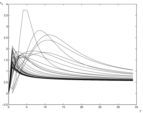
Figure 1: 38 different curves of the specific heat as a function of the temperature for $N=6$ and the following integral values of $c=2,3\ldots 39$. The dense central part of the graph are the curves obtained for the larger values of $c$ and they all resemble, except for the sharp peaks at the left, the Debye’s graph for solid crystals. The curves have very large values for the derivative at the sharp peaks and so may be suggestive of phase transition at these points. The other curves are for small $c$ and they represent the “soft” substances that have a comparable low Einstein frequencies and therefore a high values of the specific heats.

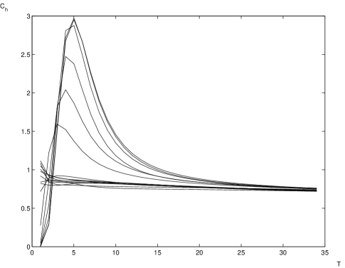
Figure 2: 15 different curves of the specific heat as a function of the temperature for $N=6$ and the following values of $c=0.3,0.4,\ldots 1.7$. The dense central part of the graph is composed of 9 similar curves obtained for the larger values of $c$ but since these values are small compared to those of Figure 1 these curves are not similar to the Debye graph. The other 6 curves are for the smaller values of $c$ and they deviate significantly from each other and from those at the center. Note that a small difference of only 0.1 in $c$ between neighbouring curves is capable of producing this large difference in appearance. Comparing this figure with the former one which has been drawn for the same $N$ but for larger values of $c$ one sees that only 3 curves out of 38 in Figure 1 deviate markedly from the dense central part.

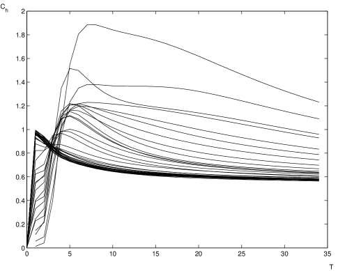
Figure 3: 39 different curves of the specific heat as a function of the temperature for $N=15$ and for the following integral values of $c=2,3\ldots 40$. As in figure 1 the dense central part of the figure are the curves that represent the Debye curve, except for the sharp peaks at the left at which the specific heats have very large values for their derivatives and so are suggestive of phase transition. Note that the curves that are not part of the central dense batch have double peaks where the first one may be seen at low $T$.

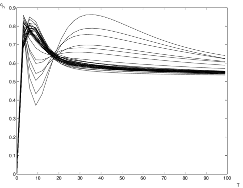
Figure 4: 39 different curves of the specific heat as a function of the temperature for $N=35$ and for the following integral values of $c=2,3\ldots 40$. As in the former figures the dense central part of the figure are the curves that represent the Debye curve, except for the sharp peaks at the left at which the specific heats have very large values for the derivatives. Note that the double peak character of the curves that are separate from the central part is more pronounced than at the former figure.

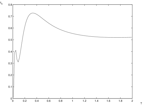
Figure 5: Double peak of the specific heat as a function of the temperature for infinite $N$ and for $c=200$. Note the difference between the heights of the two maxima and that the double peak is retained even at this large value of $c$ compared to the finite $N$ case.

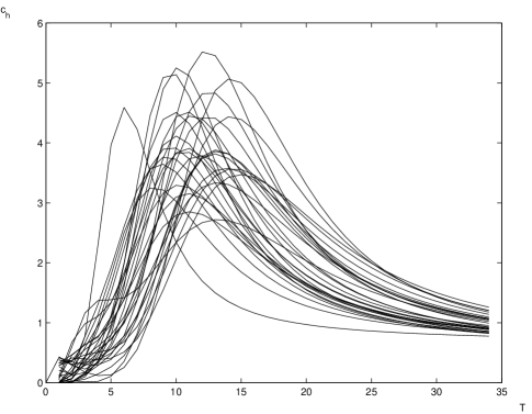
Figure 6: 30 different curves of the specific heat as a function of the temperature for infinite $N$ ans for the following values of $c=0.3,0.4,\ldots 3.2$. All the curves tend to the value of 0.55 for large $T$. The first peaks are not clearly shown for all the curves due to the large range of $T$ over which they are drawn. For smaller ranges of $T$, as in Figure 5, all the first peaks are clearly shown (not here). Note that the second peak of each curve is much larger than the first and that all these second peaks are obtained for $T>5$. The peaks of each curve have very much large values for their derivative and so they are suggestive of phase transitions.

Figure 7: 40 different curves of the specific heat as a function of the temperature for infinite $N$ ans for the following integral values of $c=2,3,\ldots 41$. Note the central dense batch of the similar figures known from finite $N$. It appears due to the large values of $c$ compared to these for which Figure 6 (and also Figure 2 for the finite $N$) was drawn which is the reason that the Debye-like form is absent in All the curves of Figure 6 (and Figure 2). Producing the curves of Figures 6 and 7 in the immediate neighbourhood of the crtical temperature $T_{c}$ demonstrate clearly the existence of their first peaks (not shown here).

References

- [1] D. Bar and L. P. Horwitz, Eur. Phys. J. B, 25, 505-518, (2002); Phys. Lett A, 296, 265-271, (2002).
- [2] "Quantum mechanics" edition by E.Merzbacher, John Wiley and sons, (1961); "Quantum mechanics" by C. C. Tannoudji, B. Diu, And Franck Laloe, John Wiley and Sons (1977)
- [3] "The transition to chaos in conservative classical systems: Quantum manifestations", L. E. Reichel, Springer, Berlin, 1992 ;E. Haller, H. Koppel and L. S. Cederbaum, Chem. Phys. Lett, 101, 215-220, (1983); T. A. Brody, J. Flores, J. B. French, P. A. Mello, A. Pandey and S. S. M. Wong, Rev. Mod. Phys, 53, 385, (1981)
- [4] "Statistical Physics" by F. Reif, McGraw-Hill book company, 1965; "Statistical Physics" by L. D. Landau and E. M. Lifshits, Oxford, Pergamon Press, (1980).
- [5] P. Fendley and O. Tchernyshyov, ArXiv cond-mat/0202129
- [6] K. -T. Lueng and Z. Neda, Phys. Lett. A, 246, 505, (1998).
- [7] Y. Tanaka, H. Tanaka, T. Ono, A. Oosawa, K. Morishita, K. Iio, T. Kato, H. A. Katori, M. I. Bartashevich and T. Goto, J. Phys. Soc. JPN, 70, 3068, (2001); P. G. Pagliuso, R. Movshovich, A. D. Bianchi, M. Nicklas, N. O. Moreno, J. D. Thompson, M. F. Hundley, J. L. Sarrao, and Z. Fisk, arXiv: Cond-Mat/0107266, v2, 2001;
- [8] B. J. Kim, P. Minnihagen, H. J. Kim, M. Y. Choi and G. S. Jeon, Europhys. Lett, 56, 222, (2001).
- [9] C. M. Ko and M. Asakawa, Nucl. Phys A, 566, 447c-458c, (1994).
- [10] "A modern course in Statistical physics" by L. E. Reichl, University of Texas Press, Austin, (1980).
- [11] K. W. Yu, Computers in Physics, 4, 176-178, (1990)
- [12] "Properties of Matter" by B. H. Flowers and E. Mendoza, John Wiley & Sons Ltd. London, (1970).
- [13] “Quantum Mechanics using Maple”, by H. Marko, Springer, Berlin, (1995).
- [14] B. Misra and E. C. Sudarshan, J. Math. Phys,18, 756, (1977); "Decoherence and the appearance of a classical world in quantum theory", D. Giulini, E. Joos, C. Kiefer, J. Kusch, I. O. Stamatescu and H. D. Zeh, Springer-Verlag, (1996); Marcus Simonius, Phys. Rev. Lett, 40, 15, 980-983, (1978); R. A. Harris and L. Stodolsky, J. Chem. Phys, 74, 4, 2145, (1981); Mordechai Bixon, Chem. Phys, 70, 199-206 (1982); Saverio Pascazio and Mikio Namiki, Phys. Rev A 50, 6, 4582, (1994); W. M. Itano, D. J. Heinzen, J. J. Bollinger, and D. J. Wineland, Phys. Rev A 41, 2295-2300, (1990); R. J. Cook, Physica Scripta T 21, 49-51 (1988); A. Peres, Phys. Rev D 39, 10, 2943, (1989); A. Peres and Amiram Ron, Phys. Rev A 42, 9, 5720, (1990); Y. Aharonov and M. Vardi, Phys. Rev D, 21, 2235, (1980); P. Facchi, A. G. Klein, S. Pascazio and L. Schulman, Phys. Lett A 257, 232-240, (1999).
- [15] A. Peres, Am. J. Phys, 48, 931-932, (1980).
- [16] D. Bar and L. P. Horwitz, Int. J. Theor. Phys, 40, 1697-1713, (2001)
- [17] D. Bar, Phys. Rev. E, 64, No: 2, 026108/1-10, (2001)
-
[18]
R. V. Smoluchowski, Z. Phys. Chem., Stoechiom.
Verwandtschaftsl, 29, 129, (1917);
"Diffusion and reactions in fractals and disordered media" by D. Ben-Avraham And S. Havlin, Cambridge, Camgridge University Press, 2000;