Simulations of the adiabatic quantum optimization for the Set Partition Problem.

Abstract

We analyze the complexity of the quantum optimization algorithm based on adiabatic evolution for the NP-complete set partition problem. We introduce a cost function defined on a logarithmic scale of the partition residues so that the total number of values of the cost function is of the order of the problem size. We simulate the behavior of the algorithm by numerical solution of the time-dependent Schrödinger equation as well as the stationary equation for the adiabatic eigenvalues. The numerical results for the time-dependent quantum evolution indicate that the complexity of the algorithm scales exponentially with the problem size. This result appears to contradict the recent numerical results for complexity of quantum adiabatic algorithm applied to a different NP-complete problem (Farhi et al, Science 292, p.472 (2001)).

1 Introduction

Most common computationally intensive tasks encountered in practice may be formulated as combinatorial optimization problems (COPs), many of which are found to belong to the algorithmic class nondeterministic-polynomial complete (NP-complete) [1]. The NP-complete problems are computationally hard - they are characterized (in the worst cases) by exponential scaling of the running time or memory requirements with the problem size. A special property of the class is that any NP-complete problem can be converted into any other NP-complete problem in polynomial time on a classical computer; therefore, it is sufficient to find a deterministic algorithm that can be guaranteed to solve all instances of just one of the NP-complete problems within a polynomial time bound.

An instance of a COP of size $n$ may be encoded using bit strings $\textsf{z}=z_{0}\,z_{1}\,\cdots\,z_{n-1}$, $\,\,z_{j}=0,1$, with a corresponding value of the cost function (or “energy”) $E=E_{\textsf{z}}$ for each string. The objective is to find the bit string(s) with the minimum cost (and the corresponding cost value). In quantum computation, bits $z_{j}$ are replaced by spin-$\frac{1}{2}$ qubits; the qubit states $|0\rangle$ and $|1\rangle$ are eigenstates of the $\pm z$ component of the $j$-th spin, respectively. The Hilbert space of a quantum register with $n$ qubits is spanned by $N=2^{n}$ basis vectors $|\textsf{z}\rangle=|z_{0}\rangle\otimes\cdots\otimes|z_{n-1}\rangle$.

2 Optimization by Adiabatic Quantum Evolution

Following [2, 3, 4], we consider a quantum evolution of duration $T$ based on the time-dependent Hamiltonian

$$H(t)=\alpha(s)\,V+\beta(s)\,H_{P},\quad s\equiv s(t).$$ (1)

Here, $H_{P}=\sum_{\textsf{z}}E_{\textsf{z}}|\textsf{z}\rangle\langle\textsf{z}|$ is the “problem” Hamiltonian that embodies the problem structure in its energy spectrum and eigenstates, the summation being performed over all $N$ $n$-bit strings, and $V$ is a “driver” Hamiltonian that is constructed in such a way as to cause transitions between those states - essentially an Ising-type spin Hamiltonian corresponding to 1- and 2-gate operations:

$$V=-\sum_{i=0}^{n-1}B_{i}\sigma_{x}^{i}-\frac{1}{2}\sum_{i,\,j=0}^{n-1}J_{ij}\sigma_{x}^{i}\sigma_{x}^{j}.$$ (2)

Coefficients $\alpha\left(s\left(t\right)\right)$ and $\beta(s(t))$ vary in time in such a way that at the initial instant of time $H(0)=V$ and at the final instant $H(T)=H_{P}$. A particular choice of the coefficients is [2]

$$\alpha(s)=1-s,\quad\beta(s)=s,\quad s(t)=t/T$$ (3)

The total Hamiltonian (1) produces a nontrivial quantum evolution from some initial (superposition) state $\psi(0)$ to a final (solution) state $\psi(T)$. If no knowledge about the solution is available a priori, then the initial state may be chosen as the symmetric state (cf. [5, 2])

$$\psi(0)=2^{-n/2}\sum_{\textsf{z}=0}^{2^{n}-1}|\textsf{z}\rangle.$$ (4)

This choice is appropriate provided (4) is a ground state of $V$ (e.g., $B_{i},J_{ij}\geq 0$). Now, if $T$ is sufficiently large, then functions $\alpha(t/T)$ and $\beta(t/T)$ vary in time slowly and the system will remain in the instantaneous (adiabatic) ground state of $H(t)$ during its entire evolution $0<t<T$ (cf. [2]). Accordingly, $\psi(T)$ will be a superposition of states $|z\rangle$ corresponding to the ground state of $H_{P}$. It is clear that in this case a measurement performed on the quantum register at $t=T$ will find with certainty one of the solutions of COP. In this case the complexity of the quantum algorithm is determined by its duration $T$. If we expand the wavefunction of the system $\psi(t)$ in the basis of the adiabatic eigenfunctions $\Psi_{k}(t)$ of the Hamiltonian $H(t)$

$$H(t)\Psi_{k}(t)=g_{k}(t)\Psi_{k}(t),\quad k=0,1,\ldots,2^{n}-1.$$ (5)

$$\psi(t)=\sum_{k=0}^{2^{n}-1}\,C_{k}(t)\Psi_{k}(t)\exp\left(-i/\hbar\int^{t}_{0}dt^{\prime}g_{k}(t^{\prime})\right),$$ (6)

then adiabatic approximation corresponds to $\psi(t)\propto\Psi_{0}(t)$ (up to the oscillating phase factor). Coefficients $C_{k}(t)$ with $k>0$ correspond to nonadiabatic corrections. Using perturbation theory in the basis of eigenfunctions $\Psi_{k}(t)$ the total probability $p_{n-ad}(t)$ of not finding the system at the instant $t$ in its adiabatic ground state equals

$$p_{n-ad}(t)=\left(\frac{\dot{s}(t)}{s(t)}\right)^{2}\,\sum_{k=1}^{2^{n}-1}\,\frac{|V_{0k}|^{2}}{[g_{k}(t)-g_{0}(t)]^{4}}$$ (8)

$$V_{0k}=\langle\Psi_{0}|V|\Psi_{k}\rangle.$$

Here we used the explicit form of coefficients $\alpha,\,\beta$ given in (3). It is seen that during the quantum evolution coefficients $C_{k}(t)\sim\dot{s}/s\sim 1/T$ and the largest admixture of the exited states into the total superposition occurs at the instant of time when one of the exited levels $g_{k}(t)$ closely approaches the ground state (avoided-crossing). From here the overall criterion for the adiabatic evolution can be expressed in the well-known form

$$\eta={\tilde{V}\over T\Delta g_{min}^{2}}\ll 1,$$ (9)

where $\Delta g_{min}$ is the closest approach of the ground state to one of the excited states during the evolution - a minimum gap- and $\tilde{V}$ is the characteristic energy scale for the matrix elements of $V$. We note that although instantaneous nonadiabatic corrections (8) are quadratic in the parameter $\eta$ (near the avoided crossing) the probability of nonadiabatic transitions $W_{n-ad}$ away from the ground state is exponentially small in $\eta$ [6]. This probability is defined on an infinite time axis and its logarithm is proportional to the imaginary part of the integral along the contour in the complex plane of $t$ that begins and ends on the real time axis and loops around the complex branching point $t^{*}$

$$W_{n-ad}~{}\exp\left(-|{\rm Im}\oint\,g_{0}(t)dt|\right).$$ (10)

Here $t^{*}$ correspond to one of the roots of the equation

$$g_{k}(t^{*})=g_{0}(t^{*})$$ (11)

that provides the smallest value for the exponential in (10) (out of all possible complex solutions of (10) for different excited states $\Psi_{k}$). In a standard (Landau-Zener) theory of nonadiabatic transitions the value of the exponent is approximately of the order of the parameter $\eta$ in (9), and therefore it is the size of the minimum gap $\Delta g_{min}$ that determines the condition for T and hence the complexity of the quantum adiabatic search algorithm according to [2]. We note finally that, as pointed out in [4], the improved complexity of the adiabatic algorithm is determined by the instantaneous rate $\dot{s}(t)/s(t)$ of the variation of the control parameter $s(t)$ near the avoided crossing. We will not discuss in this paper such modifications and focus primarily on intrinsic properties of the quantum system in question.

3 Set Partition Problem

In this paper, we will analyze the complexity of the adiabatic quantum optimization for the set partition problem (SPP), which is one of the basic NP-complete problems of theoretical computer science [1]. The optimization version of SPP is to partition a set of $n$ positive integers $\{\alpha_{0},a_{1},\ldots,\alpha_{n-1}\}$ into two disjoint subsets ${\mathcal{A}}_{1}$ and ${\mathcal{A}}_{2}$ such that the “residue” $|\sum_{\alpha_{j}\in{\mathcal{A}}_{1}}\alpha_{j}-\sum_{\alpha_{j}\in{\mathcal{A}}_{2}}\alpha_{j}|$ is minimized. The complexity of the problem substantially depends on the size of the integers $\alpha_{j}$ (see below). It is often customary for the analysis of the random instances of the problem to introduce finite-precision rational numbers $a_{j}$ that are independently and identically distributed (i.i.d.) in the unit interval $(0,1]$.

$$\alpha_{j}\leq 2^{b}\,\,\,\,\forall j,\quad a_{j}=2^{-b}\alpha_{j}\in(0,1]$$ (12)

Here $b$ is the total number of bits used to represent the numbers $a_{j}$. The values of the partition can be encoded in binaries by attaching “sign” bits $s_{j}$ to the numbers $a_{j}$. The partition residue can be defined as $|\Omega_{\textsf{z}}|$ where

$$\Omega_{\textsf{z}}=\sum_{j=0}^{n-1}s_{j}a_{j},\quad s_{j}=1-2z_{j}=\pm 1\quad(z_{j}=0,1)$$ (13)

Here $\Omega_{\textsf{z}}$ is a signed partition residue. We note that by definition the problem is symmetric: two bit strings that can be obtained from each other by flipping all the bits ($s_{j}\rightarrow-s_{j}$) correspond to two values of $\Omega_{\textsf{z}}$ that differ only in sign. We note that the minimum-residue partition(s) may be thought of as the ground state(s) of the following spin Hamiltonian [7]

$$\Omega_{\textsf{z}}^{2}=\sum_{i,\,j=0}^{n-1}a_{i}a_{j}s_{i}s_{j}.$$ (14)

This is an infinite range Ising spin glass with Mattis type antiferromagnetic coupling, $J_{ij}=-a_{i}\,a_{j}$. Infinite range coupling clearly represents a major problem with direct (‘analog’) physical implementation of this Hamiltonian on a quantum computer. Therefore one can consider using an oracle-type cost function $E(\textsf{z})=|\Omega_{\textsf{z}}|$ to implement the problem Hamiltonian in (1) for SPP. The corresponding unitary transformation will multiply the basis states $|z\rangle$ by phase factors $\exp\left(-i\Delta t\,E(\textsf{z})\right)$ during the elementary discrete steps of the ‘continuous-time’ adabatic quantum optimization (1). Although this approach is natural for the satisfiability problem [2] it has a serious limitation for SPP (as well as some other NP-complete problems like integer programming, where the precision of integers is of central importance). To demonstrate this point we need to consider the density of states of the partition residues.

3.0.1 Density of states

We define the density of states for a given instance of SPP as follows

$$\rho(\Omega)=\sum_{\textsf{z}}\delta(\Omega-\Omega_{\textsf{z}}).$$ (15)

The exact form of $\rho(\Omega)$ depends on a given instance of SPP (i.e., a particular set of numbers $a_{j}$). However we introduce a coarse-grained density of states

$${\bar{\rho}}(\Omega)=\frac{1}{\Delta\Omega}\int_{\Omega}^{\Omega+\Delta\Omega}\rho(\zeta)\mathrm{d}\zeta$$ (16)

where averaging is over an interval of $\Delta\Omega$ whose size will be determined below. Using (13) and (15) we can rewrite this expression in the form

$${\bar{\rho}}(\Omega)=\frac{2^{n}}{2\pi}\int_{-\infty}^{\infty}{e^{iw(\Omega+\Delta\Omega)}-e^{iw\Omega}\over iw}\,I(w)\,\mathrm{d}w,\quad\quad I(w)=\prod_{j=0}^{n-1}\cos(a_{j}w).$$ (17)

Note that $I(\pi k2^{b})=(-1)^{k},\,k=0,\pm 1,\ldots$ and $I(w)$ has very sharp maxima (minima) at those points. In their vicinities the integral in (17) can be evaluated by steepest descent method for any given problem instance. The sum over the contributions from different saddle points was obtained by Mertens [7] in his derivation of the partition function for the corresponding spin glass model. We emphasize however that $I(w)$ can have multiple sharp resonances at the intermediate points $|w|<2^{-b}$. The positions of these resonances are at the multiples of $\pi/q$ where $q$ is an approximate greatest common divisor (g.c.d.) of the set of $n$ numbers $a_{j}$ such that $a_{j}=f_{j}q+r_{j}$ where $f_{j}$ are integers and $r_{j}$ are residues of the division. Provided that most of the residues are sufficiently small

$${\pi^{2}\over 2}\sum_{j=1}^{p}r_{j}^{2}\leq 1,\quad p\sim n,$$

the function $I(w)$ will have steep peaks at those points. It can be shown that in the general case the value of the approximate g.c.d. for a set of $n$ $b-bit$ numbers inside the unit interval scales as $2^{-n}$ for $n<b$. Obviously it equals $2^{-b}$ for $n>b$. In what follows we will be interested in the high-precision case $n<b$. We choose the size of the averaging window $\Delta\Omega\gg 2^{-n}$ and this introduces a cut-off in the integral (14) at

$$|w|\ll\pi/\Delta\Omega\ll 2^{n}$$

It follows from above that in this case the values of the g.c.d. will lie outside the cutoff and corresponding resonances will not contribute to the integral. The value of the integral can be estimated near the single remaining maximum at $w=0$. The width of the maximum near that point is   $\delta w~{}n^{-1/2}\ll 1$ and therefore the window function in (13) works as a step function in that region. Finally we obtain

$${\bar{\rho}}(\Omega)={2^{n}\over\sqrt{2\pi n\sigma^{2}}}\exp\left(-{\Omega^{2}\over 2n\sigma^{2}}\right),\qquad\sigma^{2}=\frac{1}{n}\sum_{j=0}^{n-1}a_{j}^{2}.$$ (18)

Here the variance $\sigma$ is a “self-averaging” quantity, and the coarse-graining is performed over an interval much larger than the characteristic separation between neighboring partition residue values

$$\Delta E\,\sim\,\sqrt{n}\,\,2^{-n}$$ (19)

yet much smaller than the scale of variation of ${\rho}(\Omega)$: $\Delta E\ll\Delta\Omega\ll\sqrt{n}$. We note that in the high-precision regime ($n<b$), partition residues $\Omega_{\textsf{z}}$ are irregularly spaced and well separated from each other (on the scale of $2^{-b}$). However this structure is being averaged out in (18) and the result indicates that, in general, no more structure exists on a scale $\gg 2^{-n}$ other than that given by the Gaussian distribution in (18). We note that this distribution is usually obtained for the SPP using averaging over different instances of the problem (cf. [8, 9], [7](b)); here we recovered it as a coarse-grained distribution for a given instance which is more consistent with our goal of studying the complexity of the adiabatic quantum optimization algorithm [10].

3.1 Cost function

Computational complexity of SPP depends critically on the number of bits $b$: numerical simulations with independent identically distributed (i.i.d.) random $b$-bit numbers $a_{j}$ show [11, 12] that the solution time grows exponentially with $n$ for $2^{n-b}\ll 1$ (high-precision, computationally ‘hard phase’), and polynomially for $2^{n-b}\gg 1$ (low-precision, computationally ‘easy phase’), exhibiting a behavior similar to a phase transition [7](a).

In the low-precision phase, values of $\Omega_{\textsf{z}}$ are equally spaced (in $2^{-b}$) and strongly degenerate each corresponding to (roughly) $2^{b-n}\gg 1$ number of bit-strings. This degeneracy grows exponentially with n if $b$ remains fixed. The total number of solutions with zero residues accumulate correspondingly and this is why the complexity eventually becomes polynomial in $n$. The quantum algorithm suggested in [13] directly computes the density of states (15) of the SPP and is efficient in finding the number of solutions in the low-precision case. In this case it is also feasible to use a cost function $E(\textsf{z})=|\Omega_{\textsf{z}}|$ (provided the number of possible values does not grow exponentially with $n$).

The situation is qualitatively different in the high-precision case. Implementation of the approach based on the above cost function will require a quantum computer using exponentially high precision physical parameters (external fields, etc) to control small differences in the phases of unitary transformations on the scale at least $~{}2^{-n}$. This is a technical difference from the constraint satisfaction problem in which the cost function generally takes only the set of values that scales polynomially with $n$; the size of the set equals the total number of constraints $m$ (the computationally most difficult case corresponds to $m\sim n$ and the case of $m\sim 2^{n}$ is not of general interest there). To avoid the above restriction in the implementation of the adabatic quantum optimization algorithm for SPP, we introduce a cost function $E(\Omega)$ based on a logarithmic scale of the partition residue values:

$$E(\Omega)=0,\quad{\rm for}\quad 0\leq|\Omega|/\Delta<1,$$ (20)

$$E(\Omega)=k,\quad{\rm for}\quad 2^{k-1}\leq|\Omega|/\Delta<2^{k},\quad k=0,1,\ldots L,$$

$$2^{L-1}\leq A/\Delta<2^{L},\quad A=\sum_{j=0}^{n-1}a_{j}.$$

Since the density of states is linear at $\Omega\ll\sqrt{n}$ number of states $d_{k}$ per energy level $E(\Omega_{\textsf{z}})=k$ will grow exponentially with $k$ in that range ($\sim 2^{k}$). The total number of levels $L$ depends on the value of $\Delta$. Using the density of states (18) for $\Omega_{\textsf{z}}\ll\sqrt{n}$ one can set

$$\Delta=\sqrt{n}\,2^{-n}\,K.$$ (21)

where $K$ is some fixed number (a few dozen) independent of $n$. The number of ground states of the problem Hamiltonian

$$H_{P}=\sum_{k=0}^{L-1}E(\Omega_{z})|z\rangle\langle z|$$ (22)

approximately equals $K$, and the total number of energy levels $L$ is close to $n$. It can be estimated from (20) that $n-L\sim log_{2}{K}$. The distribution of the low-lying states $d_{k}$ with cost function (20) is somewhat similar to that in the slightly underconstrained cases of the satisfiability problem.

4 Results

To study the complexity of the adiabatic quantum optimization algorithm for SPP, we numerically integrate the time dependent Schrödinger equation with the Hamiltonian $H(t)$ (1), (2) in which we set $B_{i}=1$ and $J_{ij}=0$. We start from the symmetric initial state (4) and integrate the Schrödinger equation in the interval $0\leq t\leq T$. Unlike the approach adopted in [3] we do not set a-priori a value of success probability. Instead we introduce a complexity metric for the algorithm

$${\cal C}(T)={T+1\over p_{0}(T)}d_{0}.$$ (23)

Here $p_{0}(T)$ is the total probability of finding the system in its ground level (with $E(\Omega_{\textsf{z}})=0$) at the end of the algorithm, $t=T$, and $d_{0}$ is the number of states at the ground level. The algorithm has to be repeated on average $d_{0}/p_{0}(T)$ number of times to reach success probability $\approx$ 1. A typical plot of ${\cal C}(T)$ for an instance of SPP with $n$=15 numbers is shown in Fig. 1. At very small $T$ the wavefunction is close to the symmetric initial state and the complexity is $\sim 2^{n}$. The extremely sharp decrease in ${\cal C}(T)$ with $T$ is due to the buildup of the population $p_{0}(T)$ in the ground level as quantum evolution approaches adiabatic limit. At certain $t=T^{*}$ the function ${\cal C}(T)$ goes through the minimum: for $T>T^{*}$ the decrease in the number of trials $d_{0}/p_{0}(T)$ does not compensate anymore for the overall increase in the runtime $T$ for each trial. The minimal complexity $C^{*}=C(T^{*})$ is defined via one dimensional minimization over $T$ for a given problem instance [14].

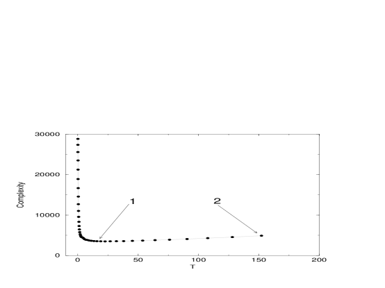
Figure 1: $C(T)$ vs $T$ for n=15, precision b=25 bits. Point 1 on the figure corresponds to the minimal value of complexity; the corresponding values are $T^{*}=22.67$, $p_{0}(T^{*})=0.15$ and $d_{0}=22$. At Point 2 the total population of the ground level has already reached $p_{0}(T)=70\%$.

In Fig.2 we plotted the data for optimal complexities $C^{*}$ at different values of $n$ on a logarithmic scale. Vertical sets of points on the plot indicate the results for all simulation data we currently have for each $n$. The results indicate that the median value of complexity $C^{*}$ scales exponentially with $n$; linear fit to the graph gives $\log C^{*}\approx 0.56\,n$. This corresponds to the scaling law $C^{*}\sim 2^{0.8\,n}$. The exponential behavior of the algorithm clearly manifests itself for the larger values of $n\geq$ 11. The scatter in the values of $\log C^{*}$ appears to decreases with $n$ however this result is probably due to the smaller number of data points available for larger $n$ values.

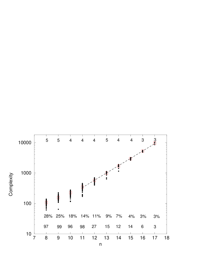
Figure 2: $C^{*}$ vs $n$, precision b=25 bits. Percentage figures correspond to the total population at the ground level at minimal complexity for a given n (e.g. 25$\%$ for n=9). Numbers below the vertical sets of points for each $n$ show the number of trials (e.g., 97 for n=8, 6 for n=16, etc). Numbers on the top indicate the average values of $d_{0}$ for all trials at a given $n$. Median values for the complexity for each $n$ are shown with red squares. The line is the least squares fit of an exponential function to the median values between n=11 and n=17.

In Fig. 3 we show the distribution of the probabilities $|\langle z|\psi(T)|^{2}$ for different values of $T$ for an instance of SPP with $n$=15 (plots for different $T$ shown with different colors)and precision b=25 bits. Values of $z$ are ordered with respect to the corresponding values of the partition residues $|\Omega_{\textsf{z}}|$. It is clearly seen on logarithmic scale that probability distribution forms ’steps’ corresponding to different values of the cost function $E(\Omega_{\textsf{z}})$ defined in (20). Within each step, the distribution of probabilities does not reveal any structure. The same property holds also for intermediate times ($t<T$). Detailed analytical results [15] indicate that it is this absence of structure in $\psi_{z}(t)$ that is responsible for the exponential complexity of the algorithm.

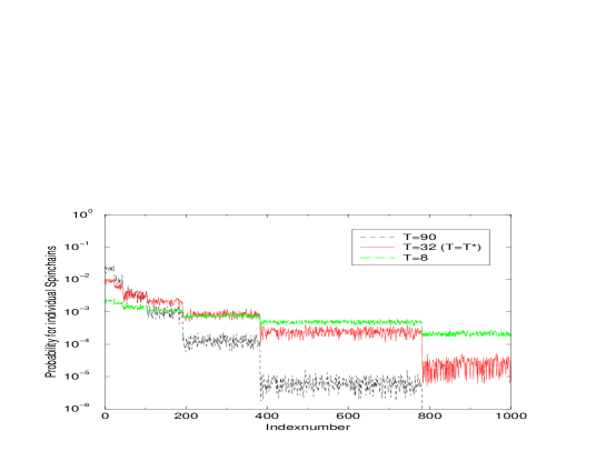
Figure 3: $|\langle z|\psi(T)|^{2}$ vs $z$ for one instance of SPP with n=15. Note that the values of the index number on the horizontal axis correspond to the positions of different bit-strings z sorted with respect to the partition residue values $|\Omega_{\textsf{z}}|$ (in increasing order). Index number 0 corresponds to the smallest partition residue. The number of states at the ground level is $d_{0}$=22. Curve shown in red corresponds to the value of $T=T^{*}=32$ (minimal complexity). Curve shown in green corresponds to the value of $T$=8 and black color curve corresponds to $T$=90.

Figure 4: Adiabatic eigenvalues $g_{k}$ vs $s=t/T$ (k=0,1,2,$\ldots$).

Figure 5: Magnified version of the Fig. 4 in the avoided -crossing region.

The Stationary Schrödinger equation

In addition to solving the time-dependent Schrödinger equation we also analyzed the adiabatic solutions of the stationary Schrödinger equation with the same form of the Hamiltonian $H(t)$ (1) as above. Our preliminary results were obtained using Mathematica for modest values of $n\leq$ 10. The results for n=10 are shown in Figs. 4 and 5. Figure 5 represents the magnified part of Fig. 4 near the avoided crossing region. Adiabatic eigenvalues were computed for different values of the scaled time parameter $s=t/T\in(0,1)$. The solid line represents the evolution of the ground state eigenvalue between $s=0$ and $s=1$. The vertical sets of points correspond to excited adiabatic levels for a given $s$. At the beginning ($s=0$) eigenvalues correspond to those of the Hamiltonian $V$: equally spaced levels -n,-n+2, $\ldots$, n, corresponding to different number of spin excitations along the $x$ quantization axis. The first excited state is $n-$fold degenerate, the second is $n(n-1)$, the k-th exited state is $\binom{n}{k}$-fold degenerate, etc. For $s>0$ the degeneracy is removed. For $s\rightarrow 1$ the eigenvalue spectrum is the one for the problem Hamiltonian $H_{P}$ (in 22). We have shifted the energy reference in the Hamiltonian $H_{P}$ by $-n$ (cf. also (1)) to match the energy scale for the symmetric case which emphasizes the avoided crossing region. In our case the ground state was 13-fold degenerate and the corresponding eigenvalues merge at $s\rightarrow 1$. The close approach of these eigenvalues is not relevant for the minimum-gap analysis since they all end up in the same final level. However the minimum separation of the instantaneous adiabatic ground state eigenvalue from the excited state eigenvalues that do not end up on the same ground level at $s=1$ is clearly seen in the figures. Note that the size of this separation is much greater than the separations between the excited states. This behavior clearly departs from the standard 2-level avoided crossing picture and is due to the contributions from the exponential number of terms in (8) as will be analyzed elsewhere [15]. We also note that the value n=10 does not correspond to the exponential scaling regime for the algorithmic complexity that appears to start for greater $n$ values as follows from the discussion above.

In conclusion, we have performed numerical simulations of the adiabatic quantum optimization for SPP using a step-like density of states defined on a logarithmic scale of partition residues. The results indicate an exponential scaling of the algorithmic complexity as a function of the problem size. The apparent reason is the loss of structure in SPP during the effective coarse-graining over the intervals of partition residues corresponding to the same cost function values.

References

- [1] M.R. Garey and D.S. Johnson, Computers and Intractability. A Guide to the Theory of NP-Completeness (W.H. Freeman, New York, 1997)
- [2] (a) E. Farhi, J. Goldstone, S. Gutmann, and M. Sipser, “Quantum computation by adiabatic evolution,” arXiv:quant-ph/0001106; (b) E. Farhi, J. Goldstone, S. Gutmann, J. Lapan, A. Lundgren, and D. Preda, “A quantum adiabatic evolution algorithm applied to random instances of an NP-complete problem”, Science 292, 472 (2001).
- [3] E. Farhi, J. Goldstone, and S. Gutmann, “A numerical study of the performance of a quantum adiabatic evolution algorithm for satisfiability,” arXiv:quant-ph/0007071; A. M. Childs, E. Farhi, J. Goldstone, and S. Gutmann, “Finding cliques by quantum adiabatic evolution”, arXiv:quant-ph/0012104.
- [4] J. Roland and N. Cerf, ”Quantum Search by local adiabatic evolution”, arXiv:quant-ph/0107015
- [5] L. K. Grover, “Quantum mechanics helps in searching for a needle in a haystack,” Physical Review Letters 79, 325–328 (1997).
- [6] L.D. Landau and E.M. Lifschitz , ”Quantum Mechanics”, Pergamon, London (1959).
- [7] S. Mertens, (a) “Phase transition in the number partitioning problem,” Physical Review Letters 81, 4281–4284 (1998); (b) “Random costs in combinatorial optimization,” Physical Review Letters 84, 1347–1350 (2000).
- [8] Y. Fu, in Lectures in the Sciences of Complexity, ed. by D.L. Stein (Addison-Wesley Publishing Company, Reading, Massachusetts, 1989).
- [9] F. Ferreira and J. Fontanari, Journal of Physics A 31, 3417 (1998).
- [10] We also note that occasionally for certain ”singular” instances of the partition problem values of approximate g.c.d. can be rather large (e.g. ), i.e. most of the numbers are nearly commensurate with each other. In this case intermediate resonances will be of interest and the density of states will have an additional structure at low ’frequencies’ . We do not consider those instances in a present paper.
- [11] I.P.Gent and T. Walsh, Comp. Intell. 14, 430 (Blackwell, Cambridge MA, 1998).
- [12] R.E. Korf, Artif. Intell. 106, 181 (1998).
- [13] H. De Raedt et al,Phys. Lett. A 290,5-6, p. 227-233 (2001).
- [14] We note that an additional optimization can be done if one defines a complexity similar to (23) but uses an intermediate time instance instead of there. In this case quantum algorithm is terminated at the instance for each when minimal complexity is reached and then additional minimization over is performed. Our results indicate that this method does provide further improvement for the overall complexity but takes a prohibitely long time to perform numerical optimization of .
- [15] V.N. Smelyanskiy, U.V. Toussaint, D.A. Timucin, to be submitted.