A perspectival version of the modal interpretation of quantum mechanics and the origin of macroscopic behavior

Abstract

We study the process of observation (measurement), within the framework of a ‘perspectival’ (‘relational’, ‘relative state’) version of the modal interpretation of quantum mechanics. We show that if we assume certain features of discreteness and determinism in the operation of the measuring device (which could be a part of the observer’s nerve system), this gives rise to classical characteristics of the observed properties, in the first place to spatial localization. We investigate to what extent semi-classical behavior of the object system itself (as opposed to the observational system) is needed for the emergence of classicality. Decoherence is an essential element in the mechanism of observation that we assume, but it turns out that in our approach no environment-induced decoherence on the level of the object system is required for the emergence of classical properties.

Modal interpretations (see, e.g., bene ; dieks&vermaas ; bacciagaluppi2 ; bub ; vermaas&dieks ) aim at assigning properties (or states that represent these properties in a one-to-one way) to physical systems on the basis of the standard quantum mechanical formalism, though stripped from the postulates that attribute a special role to measurements. The motivation for introducing states that correspond to physical properties is the wish to give descriptions of systems, and thus to transcend the traditional interpretational framework in which systems are only discussed in terms of possible measurement results. The removal of the measurement postulates has the same background. We want to treat measurements as ordinary physical interactions, and measurement outcomes as properties of measuring devices or displays, and thus to remove any mysterious aspects of the concept of quantum measurement. As a first step towards this goal we assume all time evolution in Hilbert space to be unitary, so that there is no collapse of the wave function.

The modal approach based on these starting-points has proved to be appealing and successful when applied to situations in which the Hilbert spaces are finite and the number of dimensions is not too large bacciagaluppi and hemmo . However, in the case of continuous model systems, like freely moving particles or harmonic oscillators (assumed to be interacting with the environment), the existing prescriptions are not guaranteed to lead to the expected classical properties. In particular, one such model study bacciagaluppi has failed to demonstrate more or less sharp localization of a particle in circumstances in which one would expect a classical description to be applicable. (As for other kind of difficulties - not to be considered here - see Vermaas_no_go .) The essence of the failure to produce localization is not the continuity of the model, since the difficulty persists in models in which the Hilbert space has a finite but large dimensionality. This can be clearly seen in computer simulations, in which one always works with finite Hilbert spaces.

At present it is not clear whether in more realistic models the situation will improve and classical properties will result. Nevertheless, it seems to be worth considering - still within the modal scheme - another possibility, namely, that the observed classical properties are inevitable and generic consequences of the observation itself, but need not be present in the absence of observations. As already emphasized, we consider observations and measurements as ordinary physical interactions between object system and measuring device, and treat them quantum mechanically.

It is indeed a-priori not implausible that applying the modal scheme to the perceptual system itself will lead to results that are in accordance with experience. The reason is that our nerve system has an inherent discreteness, both in its spatial structure (cells) and in its functionality (a nerve cell either fires or does not fire). It is this kind of discreteness which seems to be needed to recover the expected classical alternatives within a quantum mechanical treatment bacciagaluppi and hemmo . Here, we will make a detailed investigation of the implications of such a discreteness in a simple model (which can be conceived either as a model of a digital measuring device or as a very crude model of a part of the nerve system). The result is that according to this model an observer looking at an object will see the object localized: from the point of view of the observer the object is localized. However, it turns out that the object is delocalized from a different perspective.

The wider question addressed in this paper is whether these (and similar) results can be fitted into a consistent and satisfactory picture. An object cannot be both localized and delocalized, so that it seems that inconsistency threatens. However, we will propose, and to some extent develop, an interpretational scheme (a generalisation of the Dieks-Vermaas modal interpretation) according to which it is not contradictory to assign such seemingly conflicting properties to an object. In this ‘perspectival’ version of the modal interpretation properties of physical systems have a relational character and are defined with respect to another physical system that serves as a reference system bene . It is important to emphasize already now that the core idea of this new conceptual scheme is that the different descriptions, given from different perspectives, are equally objective and all correspond to physical reality. Because of the relational character of the descriptions this involves no contradiction. A contradiction would only arise if different descriptions would be given from one perspective, or from compatible perspectives that can be combined into one. This will not happen in the interpretation that we will propose. Furthermore, we will show that different observers observing the same object will agree about the results, just as in classical physics (provided, of course, that the observations do not change the object).

We shall also consider the time evolution of a macroscopic object and study when and why the classical description becomes applicable. Finally, we discuss the role of environment induced decoherence.

I A perspectival version of the modal interpretation

The approach we are going to explain is closely related to the Dieks-Vermaas version of the modal interpretation: the same type of rules are used to assign properties to physical systems. But instead of the usual treatment in which properties are supposed to correspond to monadic predicates, we will propose an analysis according to which properties have a relational character.

Physical systems of a given kind are described within a characteristic Hilbert space; we will allow arbitrary Hilbert spaces. In our perspectival approach the state of a physical system $S$ (corresponding to physical characteristics of $S$) needs the specification of a ‘reference system’ $R$ with respect to which the state is defined. This reference system is a larger system, of which $S$ is a part. As already mentioned, we will allow that one and the same system, at one and the same instant of time, can have different states with respect to different reference systems. However, the system will have one single state with respect to any given reference system. This state of $S$ with respect to $R$ will be denoted by $\hat{\rho}^{S}_{R}$. It is a density matrix, i.e., a Hermitian operator acting on the Hilbert space of $S$ that is positive semidefinite and has unit trace. In the special case in which $R$ coincides with $S$ the state is in general (i.e., if there is no degeneracy, see below) a one-dimensional projector

$$\hat{\rho}^{S}_{S}=|\psi_{S}><\psi_{S}|$$ (1)

This state $\hat{\rho}^{S}_{S}$ (or equivalently $|\psi_{S}>$), the ‘state of $S$ with respect to itself’, is the same as ‘the physical state’ assigned to $S$ in the Dieks-Vermaas version of the modal interpretation; i.e. it is one of the projectors occurring in the spectral decomposition of the reduced density operator of $S$, and $|\psi_{S}>$ is one of the eigenvectors, if there is no degeneracy—see dieksy for these ideas.

The rules for determining all states, for arbitrary $S$ and $R$, are as follows. If $U$ is the whole universe, then $\hat{\rho}^{U}_{U}$ is taken as the quantum state assigned to $U$ by standard quantum theory. If system $S$ is contained in system $A$, the state $\hat{\rho}^{S}_{A}$ is defined as the density operator that can be derived from $\hat{\rho}^{A}_{A}$ by taking the partial trace over the degrees of freedom in $A$ that do not pertain to $S$:

$$\hat{\rho}^{S}_{A}={\rm Tr}_{A\setminus S}\;\hat{\rho}^{A}_{A}$$ (2)

Any relational state of a system with respect to a bigger system containing it can be derived by means of Eq.(2).

We already saw that for an arbitrary system $S$, contained in the universe $U$, $\hat{\rho}^{S}_{S}$ is postulated to be one of the projectors contained in the spectral resolution of $\hat{\rho}^{S}_{U}$. If there is no degeneracy among the eigenvalues of $\hat{\rho}^{S}_{U}$ these projectors are one-dimensional and the state can be represented by a vector $|\psi_{S}>$, see Eq.(1); in the case of degeneracy the state of the system with respect to itself is a multi-dimensional projector. For simplicity we will in the following focus on the non-degenerate case and assume that the state of $S$ with respect to itself is given by one of the eigenvectors $|\varphi^{S}_{j}>$ of $\hat{\rho}^{S}_{U}$.

The state $\hat{\rho}^{U}_{U}$ evolves unitarily in time. Because there is no collapse of the wave function in our approach, this unitary evolution of the total quantum state is the main dynamical principle of the theory. Furthermore, we assume that the state assigned to a closed system $S$ undergoes a unitary time evolution

$$i\hbar\frac{\partial}{\partial t}\hat{\rho}^{S}_{S}=\left[\hat{H}_{S},\;\hat{\rho}^{S}_{S}\right]$$ (3)

As always in the modal interpretation, the theory specifies only the probabilities of the various possibilities (the interpretation is indeterministic): the probability that $|\psi_{S}>$ is the eigenvector $|\varphi^{S}_{j}>$ is given by the corresponding eigenvalue of $\hat{\rho}^{S}_{U}$. If the systems $S_{1}$, $S_{2}$, … $S_{n}$ are pair-wise disjoint and $U$ is the whole Universe, then the joint probability that $|\psi_{S_{1}}>$ coincides with $|\varphi^{S_{1}}_{j_{1}}>$, $|\psi_{S_{2}}>$ coincides with $|\varphi^{S_{2}}_{j_{2}}>$,…, $|\psi_{S_{n}}>$ coincides with $|\varphi^{S_{n}}_{j_{n}}>$, is given by

$$P(j_{1},j_{2},...j_{n})={\rm Tr}\left(\hat{\rho}^{U}_{U}\Pi_{i=1}^{n}|\varphi^{S_{i}}_{j_{i}}><\varphi^{S_{i}}_{j_{i}}|\right)$$ (4)

We do not define joint probabilities if the systems are not pair-wise disjoint. This is in accordance with the no-go theorem by Vermaas Vermaas_no_go . More generally, joint probabilities cannot always be defined within the present approach because states that are defined with respect to different quantum reference systems need not be commensurable. In fact, this plays a significant role in demonstrating that in our approach the violation of Bell inequalities can be attributed solely to the failure of the traditional concept of reality, and does not involve nonlocality (see below, and Bene2 ).

If a system and its complement are concerned, a simple calculation based on the Schmidt representation of the state $|\psi_{U}>$ and Eq.(4) shows that the states of $|\psi_{A}>$ and $|\psi_{U\setminus A}>$ are uniquely correlated. (This result played an important role in earlier versions of the modal interpretation.) Therefore, knowledge of $|\psi_{U\setminus A}>$ is equivalent to knowledge of $|\psi_{A}>$. This suggests that one may consider the state of $S$ with respect to the reference system $A$, $\hat{\rho}^{S}_{A}$, alternatively as being defined from the perspective $U\setminus A$ (here $A$ is an arbitrary quantum reference system, while $U$ is again the whole universe). Sometimes this concept of a ‘perspective’ is intuitively more appealing than the concept of a quantum reference system (cf. Rovelli ). Nevertheless, there are some limitations inherent in this alternative. First, if $A$ itself is the whole universe, the concept of an external perspective cannot be applied. Moreover, the state of the system $U\setminus A$ in itself does not contain sufficient information to determine the state of system $A$; one also needs the additional information provided by $|\psi_{U}>$ in order to compute $|\psi_{A}>$. But $|\psi_{A}>$ does contain all the information needed to calculate $\hat{\rho}^{S}_{A}$ (cf. Eq.(2)). We will therefore relativize the states of $S$ to reference systems that contain $S$, although we shall sometimes—in cases in which this is equivalent— also speak about the state of $S$ from the perspective of the complement of the reference system.

Of course, we must address the question of the physical meaning of the states $\hat{\rho}^{S}_{A}$. In our approach it is a fundamental assumption that basic descriptions of the physical world have a relational character, and therefore we cannot explain the relational states by appealing to a definition in terms of more basic, and more familiar, non-relational states. But we should at the very least explain how these relational states connect to actual experience. Minimally, the theory has to give an account of what observers observe. We postulate that experience in this sense is represented by the state of a part of the observer’s perceptual apparatus (the part characterized by a relevant indicator variable, like the display in our simple model) with respect to itself. More generally, the states of systems with respect to themselves correspond to the (monadic)properties assigned by the earlier, non-perspectival, version of the modal interpretation.

As we shall illustrate, the empirical meaning of many other states can be understood and explained - by using the rules of the interpretation - through their relation to these states of observers, measuring devices, and other systems, with respect to themselves.

II A model of the measurement

The simple model we are going to use is sketched in Fig.1.

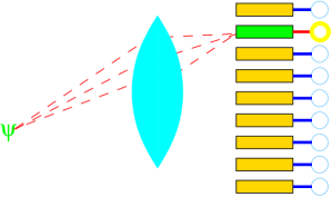
Figure 1: Sketch of the model system

The right hand side part of the drawing represents a digital measuring device. It consists of several individual blocks that do not interact with each other (as a representation of the situation in the nerve system this is a strong simplification, though part of the perceptual system can be modelled this way, especially in situations in which the incoming stimulus has a low intensity). The blocks are assumed to be very close to each other and their diameters are larger than but comparable to the wavelength of light. (The diameters of the rods and cones in the human retina are 1-2 $\mu$m). Each block consists of a receptor (drawn as a small rectangle) and a display (drawn as a circle). The operation of a receptor may be described roughly by means of two states, one corresponding to the receptor being excited, the other the ‘ready-to-measure’ state. We shall denote these by $|1>^{R}$ and $|0>^{R}$, respectively. Any superposition of these states is also allowed. A basis in the Hilbert space of the total measuring device consisting of $N$ receptors is given by the states ${\Pi_{j=1}^{N}}|i_{j}>^{R}$, in which ${}^{\prime}i_{j}^{\prime}$, referring to the $j$-th receptor, can be 0 or 1. The displays have corresponding states that we denote by $|1>^{D}$ and $|0>^{D}$ for an individual display, and by ${\Pi_{j=1}^{N}}|i_{j}>^{D}$ for the whole set of displays.

To make the ideas clear we shall assume that the interaction between the receptors and displays is such that if the $j$-th receptor is excited, and its state accordingly becomes $|1>^{R}$, then the $j$-th display will with certainty end up in the corresponding indicator state $|1>^{D}$. In other words, the receptor-display system accomplishes an ideal von Neumann measurement. This is known to be approximately realizable. In the last section of this paper we will investigate a more refined form of the model, in which the degeneracy of the just-mentioned receptor and display states is taken into account.

The just-mentioned assumption immediately implies that an arbitrary measurement leads to the entangled state

$$\sum_{\{i_{j}\}}c_{i_{1},i_{2},...,i_{N}}|\Psi_{i_{1},i_{2},...,i_{N}}>\otimes{\Pi_{j=1}^{N}}|i_{j}>^{R}\otimes|i_{j}>^{D}$$ (5)

of the whole model system, where the states $|\Psi_{i_{1},i_{2},...,i_{N}}>$ of the measured object+environment system are normed but not necessarily mutually orthogonal. Due to the one-to-one relationship between the orthonormal states ${\Pi_{j=1}^{N}}|i_{j}>^{R}$ and ${\Pi_{j=1}^{N}}|i_{j}>^{D}$, the reduced density matrix of the display system is

$$\sum_{\{i_{j}\}}|c_{i_{1},i_{2},...,i_{N}}|^{2}{\Pi_{j=1}^{N}}|i_{j}>^{D}\mbox{ }^{D}\mbox{}<i_{j}|\;,$$ (6)

i.e., it is diagonal in the ‘definite display result’ basis. Its eigenstates (except in case of degeneracy, i.e. exact equality of the squared coefficients in (6)) are the elements ${\Pi_{j=1}^{N}}|i_{j}>^{D}$ of the display result basis.

A basic principle of our interpretation is that the eigenstates of the reduced density matrix are the ‘states of the system with respect to itself’ and correspond to possible physical properties of the system (in the same way as the states assigned in the earlier versions of the modal interpretation did). One of these possibilities will be actually realized, and the probability for any particular eigenstate of representing the actual state of affairs is given by the value of the corresponding eigenvalue of the reduced density matrix. It can thus be concluded from Eq.(6) that the observation has a definite result corresponding to one of the display states. As stressed before, in the perspectival approach this definite property is represented by the state of the display with respect to itself—this leaves it open that the state and the corresponding properties may be different if relativized to another reference system. Below we will indeed encounter an example of such a difference in state ascriptions corresponding to different perspectives.

At this point we can already make a brief remark about the role of decoherence. In the model the environment of the display system is the receptor system, while coupling to the rest of the world is neglected. Therefore, environment-induced decoherence in the usual sense does not play a role here, although entanglement between receptors and displays is essential. In other words, the display states are ‘decohered’ by their correlation with the mutually orthogonal receptor states.

That a measurement, performed with a given device, invariably leads to one of a number of alternatives that are determined by the nature of the device and are independent of the measured object (the latter determines only the probability that a particular outcome occurs) has always been a standard assumption in quantum measurement theory. In the present treatment we derive this assumption from the modal approach applied to our specific model of the measuring device. It should be noted that we did not presuppose classical features of the device; the whole model is treated quantum mechanically.

Suppose that a single photon is scattered from the object. If the object possesses a large mass, we may neglect the back reaction (recoil), so the total wave function of object and photon after the scattering is of the form

$$\int dx\int dx_{e}\int dx_{ph}\Psi(x,x_{e})\varphi(x_{ph},x)$$

$$\times|x>\otimes|x_{e}>\otimes|x_{ph}>$$ (7)

In this equation $x$ stands for the position of the object, whereas $x_{e}$ and $x_{ph}$ denote the degrees of freedom of the environment and the photon, respectively. After the photon has been absorbed in one of the receptors, the state of the complete system (including the receptors and the displays) is

$$\int dx\int dx_{e}\Psi(x,x_{e})|x>\otimes|x_{e}>$$

$$\otimes\sum_{j=1}^{N}c_{j}(x)\Pi_{i=1}^{N}|\delta_{i,j}>^{R}\otimes|\delta_{i,j}>^{D}$$ (8)

In this equation $c_{j}(x)$ is the amplitude that the photon which has been scattered from $x$, in the situation depicted in Fig. 1, is absorbed at a later time in the $j$-th receptor. The amplitude is negligible unless the position of the $j$-th receptor is near the geometrical optical image of the point $x$. It follows that the reduced density matrix of the display system is given by

$$\sum_{j=1}^{N}\int dx\rho(x,x)|c_{j}(x)|^{2}\Pi_{i=1}^{N}|\delta_{i,j}>^{D}<\delta_{i,j}|^{D}$$ (9)

Here

$$\rho(x,x^{\prime})=\int dx_{e}\Psi(x,x_{e})\Psi^{*}(x^{\prime},x_{e})$$ (10)

stands for the reduced density matrix of the object in coordinate representation, still before the object is exposed to the light. Due to the recoil-free nature of the interaction, the diagonal elements $\rho(x,x)$ are not influenced by the light scattering (compare Eq.(13) below). Therefore, according to the modal scheme the actual physical condition of the display system (its state with respect to itself) is

$${\Pi_{i=1}^{N}}|\delta_{i,j}>^{D}$$ (11)

with probability

$$\int dx\rho(x,x)|c_{j}(x)|^{2}$$ (12)

Note that Eq. (9) is a special case of Eq. (6), thus Eq. (11) actually follows from the previous general considerations.

In a more general treatment, we should also take into account that the particle experiences a back-reaction because of its interaction with the photon. Instead of Eq.(8), we then have

$$\int dx\int dx_{e}\Psi(x,x_{e})|\xi_{x}>\otimes|x_{e}>$$

$$\otimes\sum_{j=1}^{N}c_{j}(x)\Pi_{i=1}^{N}|\delta_{i,j}>^{R}\otimes|\delta_{i,j}>^{D}$$ (13)

Here the states into which the position states $|x>$ are transformed by the recoil are denoted by $|\xi_{x}>$; these states are not necessarily mutually orthogonal. The probability of the j-th display being excited now becomes

$$\left|\left|\int dx\int dx_{e}\Psi(x,x_{e})\;c_{j}(x)|\xi_{x}>\otimes|x_{e}>\right|\right|^{2}$$

$$=\int dx\int dx^{\prime}\rho(x,x^{\prime})\;c_{j}(x)c^{*}_{j}(x^{\prime})<\xi_{x^{\prime}}|\xi_{x}>$$ (14)

Since the states $|\xi_{x}>$ are in general not mutually orthogonal, non-diagonal elements of the reduced density matrix of the object enter the expression. If the recoil is negligible, one has $|\xi_{x}>=|x>$ and Eq.(12) is recovered.

It is instructive to calculate the reduced density matrix $\tilde{\rho}(x,x^{\prime})$ of the object (state of the object with respect to the whole system) after it has been exposed to light, but still before the absorption of the photon in the receptors. Using Eq. (7) one obtains

$$\tilde{\rho}(x,x^{\prime})=\rho(x,x^{\prime})\int dx_{ph}\varphi(x_{ph},x)\varphi^{*}(x_{ph},x^{\prime})$$ (15)

After the absorption of the photon in the receptors one gets the same result because the time evolution during the absorption is unitary and the object degrees of freedom are not involved in the interaction. A calculation based on Eq. (8) gives the alternative expression

$$\tilde{\rho}(x,x^{\prime})=\rho(x,x^{\prime})\sum_{j=1}^{N}c_{j}(x)c_{j}^{*}(x^{\prime})$$ (16)

The equality of expressions (15) and (16) gives a condition the ‘transfer functions’ $c_{j}(x)$ must satisfy.

According to the modal interpretations one of the eigenstates of $\tilde{\rho}(x,x^{\prime})$ represents the state of the object with respect to itself (this is the physical state of the object according to the terminology of the Dieks-Vermaas modal interpretation). In general, these eigenstates are not localized bacciagaluppi , so they do not correlate with the result of the observation, which indicates a definite position.

The question naturally arises what state the observation then corresponds to. According to the modal scheme the answer follows from the biorthogonal decomposition of the state of the whole system (note that Eq.(8) is already of this form). Thus, the observation is perfectly correlated to the state of the object+environment+receptor system with respect to itself. In other words, from the perspective of $D$ all information about the object state is contained in the relational state of the object with respect to object+environment+receptor. Direct calculation based on Eq.(8) yields for this object state from the perspective of $D$:

$$\rho^{O}_{U\setminus D}(x,x^{\prime})=\frac{c_{j}(x)\rho(x,x^{\prime})c_{j}^{*}(x^{\prime})}{\int dx|c_{j}(x)|^{2}\rho(x,x)}$$ (17)

In this equation the superscript $O$ refers to the object, and the subscript $U\setminus D=O+E+R$ to the reference system, which is the complement of the system $D$ defining the perspective.

Owing to the properties of the amplitudes $c_{j}(x)$, for a given $j$ the expression (17) will be appreciable only if $x$ and $x^{\prime}$ are located in a small interval (from which light will be scattered to the $j$-th receptor). This means that the object is indeed localized from the point of view of $D$ (or, equivalently, with respect to—considered as part of—$O+E+R$). It should be noted that the form of the state of $O+E+R$ is determined by the interaction constituting the observation that took place. Without the observation we could not speak of localization as a relational property of the object.

The example illustrates how different properties may be ascribable to an object from different perspectives. In this case, the state of the object with respect to itself is not localized. However, if the complement of the display system is chosen as the reference system, a description in terms of a localized state does apply. Both descriptions are objective, but relational; they involve the specification of different reference systems. An analogy may be helpful to see that the relational character of descriptions does not entail a lack of objectivity. According to the special theory of relativity one and the same object can be described as moving or as resting, without the implication that one of these descriptions is more fundamental than the other. Both descriptions are entitled to be called objective, but make use of different ‘perspectives’. The ascription of properties in our interpretation of quantum mechanics has a similar relational character.

We will now consider a situation in which two or more measurements are performed on the same object, by means of two different measuring devices. We know from everyday experience that the results of such measurements will (more or less) agree. Our traditional notions concerning physical reality (in particular, the idea that the properties of objects are independent of any perspective and can be represented by non-relational, monadic, predicates) are to a large extent based on this and similar facts of experience. It is therefore important to show that our perspectival approach is in accordance with this agreement among observers (or measuring devices).

For simplicity we assume that the two devices are at the same position and do not disturb each other. In this way we ensure that both measurements take place under identical circumstances. Analogously to Eq.(8), the state of the compound system consisting of object, first device, and second device will after the measurement be given by

$$\int dx\int dx_{e}\Psi(x,x_{e})|x>\otimes|x_{e}>$$

$$\otimes\sum_{j=1}^{N}c_{j}(x)\Pi_{i=1}^{N}|\delta_{i,j}>^{R_{1}}\otimes|\delta_{i,j}>^{D_{1}}$$

$$\otimes\sum_{k=1}^{N}c_{k}(x)\Pi_{l=1}^{N}|\delta_{l,k}>^{R_{2}}\otimes|\delta_{l,k}>^{D_{2}}$$ (18)

If we determine from this the state of the first display system with respect to itself, we find

$${\Pi_{i=1}^{N}}|\delta_{i,j}>^{D_{1}}$$ (19)

with probability

$$\int dx\rho(x,x)|c_{j}(x)|^{2}$$ (20)

Similarly, the state of the second display system with respect to itself is

$${\Pi_{l=1}^{N}}|\delta_{l,k}>^{D_{2}}$$ (21)

with probability

$$\int dx\rho(x,x)|c_{k}(x)|^{2}$$ (22)

According to the standard rules of the modal interpretation (bene ; dieksx , see Eq.(4) ) the joint probability that the state of the first display system with respect to itself is given by Eq.(19) and the state of the second display system with respect to itself is given by Eq.(21) is

$$\int dx\rho(x,x)|c_{j}(x)|^{2}|c_{k}(x)|^{2}$$ (23)

This expression has the same form as the joint probability distribution predicted by classical theory for a situation in which independent measurements are made on each member of an ensemble of systems distributed in space with probability density $\rho(x,x)$. The properties of the coefficients $c_{j}(x)$ imply that the expression (23) vanishes unless $j\approx k$. Indeed, $c_{j}(x)$ is practically zero unless the $j$-th receptor block is situated near (i.e., in a distance of few wavelengths) of the geometrical optical image of $x$. Therefore, our interpretational scheme predicts that two observers looking at the same macroscopic object, at the same time and under identical circumstances, will see it (practically) in the same place. We assumed in the calculation that the interaction between the photon and the object was recoil-free; this is justified in the case of a macroscopic object. We have already seen that if recoil should be taken into account, off-diagonal elements $\rho(x,x^{\prime})$ from the narrow band in the matrix where $c_{j}(x)$ and $c_{j}(x^{\prime})$ are both appreciably different from zero will enter the expression for the probability of the j-th receptor being excited. Moreover, if there is substantial recoil the second measurement will show a different result than the first, because of the disturbance caused by the first measurement. This is not different from what would happen according to classical physics.

In expression (23) it does not matter whether the system was in a pure or mixed state prior to the measurement. Therefore, in our analysis of the observational mechanism macroscopic objects will be observed as localized quite independently of whether decoherence of the object state by interaction with its environment has taken place. Our analysis indicates that this point generalizes to arbitrary observation mechanisms that possess the characteristic finiteness and determinism assumed in our model. This result brings to light an important difference between our approach, in which features of the measurement process take a central role, and approaches according to which the localization of macroscopic objects is due to environment-induced decoherence of the object state. As emphasized before, according to the modal interpretation environment-induced decoherence will in general not guarantee that a macroscopic object will be localized (in the sense that its state with respect to itself is localized), because of the lack of localization of the eigenstates of the object’s reduced density matrix.

A similar analysis applies to the case in which the measurement is repeated, possibly many times and in rapid succession, by means of the same device. An adequate mathematical treatment of that case includes the description of a memory which stores the result of the first measurement (this memory would be analogous to the first display system in the above situation) and a mechanism which resets the measuring device and prepares it for the next measurement. Without discussing the details, we just mention that the results (especially the counterpart of Eq.(23)) are completely analogous.

III The notion of physical reality in the perspectival approach

Although the agreement between different observers, which fits in naturally with the classical notion of physical reality and may even seem to imply it, was just found to be present in our interpretation of the quantum formalism as well, the overall picture of physical reality that emerges is very different from the usual one. A good starting-point for an explanation of the differences is a discussion of the applicability of the Einstein-Podolsky-Rosen reality criterion. This criterion says that

If, without in any way disturbing a system, we can predict with certainty (i.e., with probability equal to unity) the value of a physical quantity, then there exists an element of physical reality corresponding to this physical quantity.EPR .

Let us see how this applies to the just-discussed measurement situation, in which the object interacts with the impinging photons, which is followed by an interaction between the scattered photons and the receptors, after which there finally is an interaction between the displays and the receptors. The whole process is repeated in the second measurement. The result shown by the first display system allows an (almost) certain prediction of the result of the second measurement. The question is what we can say about the state of the object, after the light has been scattered for the first time, on the basis of the EPR-criterion.

The interactions between the photons and the receptors and between the receptors and the displays obviously do not disturb the object, which may find itself at a large distance. As soon as the display shows a result (or if the result is read off, but we prefer to avoid the introduction of a conscious observer), there is a one-to-one relation with the result of the second measurement. In other words, the result of the second measurement is predicted, with certainty, by the result of the first measurement. As we have seen, the prediction is that the system will be found at a definite position. At first sight, the EPR-criterion therefore seems to imply that the object system already possessed a definite position from the moment it interacted with the photons.

However, in the approach that we are explaining things are not so straightforward. In our scheme, the physical quantity that is predicted corresponds to a relational state of the object, namely its state with respect to the object+environment+receptor system (cf. Eq.(17)). Now, the important point is that the first measurement has given rise to the perspective from which it is possible to make this prediction. Therefore, although it is true that there was no physical interaction between the display and the object, the display nevertheless plays a part in determining the object state with respect to object+environment+receptor (which is the complement of the display system itself). The physical interaction with the display affected the reference system, and therefore influenced the relational state.

The fact that the relevant states have this relational (perspectival) character is responsible for the failure of ordinary counterfactual reasoning: from the fact that no physical disturbance has affected the object, it cannot always be concluded that the object state has remained the same. One should also look at the reference system, with respect to which the state is defined, and see whether anything has changed there that is relevant.

Einstein, Podolsky and Rosen thought it very unlikely that the quantities of an object system would depend on whether or not a remote measurement is performed. Within the conceptual framework of classical physics, in which properties attach to an object as monadic (non-relational) predicates, this skepticism is completely justified. However, in our present framework the possibility of the dependence in question naturally appears, not as an effect of physical disturbances acting on the object but as a consequence of a change in the conditions that define the perspective. This change comes about by local physical influences on the quantum reference system.

This line of reasoning is in accordance with Bohr’s qualitative arguments that any reasonable definition of physical reality in the realm of quantum phenomena should also include the experimental setup Bohr . In the present relational approach states of a system are defined with respect to any larger physical system, so the concept of reality is not exclusively connected to the presence of instruments. Nevertheless, in our scheme too, observed reality contains elements relating to us as observers in an essential way: we define the perspective. However, this does not imply any subjectivism. The various relational states follow unambiguously from the quantum formalism, and the way the world should be described depends accordingly on objective physical features (whether or not the observing system is discrete, the nature of the interaction, whether the object has a large mass, and so on).

These considerations show how the very concept of reality is modified in our interpretation of quantum mechanics. The essential new point is that quantum properties and quantum states possess a relational character. In general, one may expect that this quantum feature will not be noticeable on the level of observations, because of the agreement between different observers. Yet, the modification persists even in the macroscopic domain. As we saw, the observed localization of macroscopic objects is absent from a different perspective. And on the observational level, Bell-type experiments reveal the untenability of the traditional notions of reality (monadic properties combined with locality).

Let us return to the EPR reality criterion and draw conclusions about its status within our conceptual framework. As it stands, the criterion is ambiguous (as observed by Bohr in his reply to Einstein, Podolsky and Rosen), since nothing is said about the perspective from which the physical quantity whose value can be predicted is defined. If the reference system is specified, the criterion is valid if neither the described system nor the quantum reference system is disturbed. That is, if it is possible to predict a relational state without any changes either in the reference system or the object, the state is there (as a part of physical reality) independently of whether or not the prediction is made.

Specifically, one could understand the EPR-criterion as referring to the state of the system with respect to itself. In this case, the well-known ‘no-signaling’ theorem becomes relevant: a system’s density matrix (found by partial tracing from $\hat{\rho}^{U}_{U}$), and therefore its eigenstates, will not change as a result of things happening elsewhere (remember that we do not have collapses of the wave function in our scheme). So, if it is possible to predict the state of a far-away particle (w.r.t. itself) on the basis of measurements performed elsewhere, we surely should conclude that that state existed independently of those measurements, and the EPR criterion therefore holds.

Let us now apply the EPR reality criterion to the case for which it was devised, the case of distant correlated particles. We find that the state of the second particle that becomes precisely known after a measurement on the first particle, is the state of this second particle with respect to the two-particle system (i.e., the state from the perspective of the measuring device). However, it cannot be concluded that this state was already present before the measurement, because the state of the reference system w.r.t. itself (from which the state of particle 2 w.r.t. this reference system is derived) was changed by the measurement. If one writes down the states explicitly, applying the given rules to the situations before and after the measurement, one easily establishes that the state of particle 2 w.r.t. the two-particle system indeed changes as a result of the measurement, in spite of the fact that there was no mechanical disturbance of particle 2.

By contrast, the state of particle 2 with respect to itself does not change and there is no influence on the reference system. So, if the state of particle 2 with respect to itself can be predicted from the result of the first measurement, application of the EPR criterion is possible and yields a result which is in harmony with quantum mechanics (in our interpretation): the state of particle 2 w.r.t. itself was indeed an element of physical reality already before, and independently of, the measurement on particle 1. More generally, although the EPR criterion can be upheld within our conceptual framework (by specification of the missing reference system), its application does not lead to the conclusion that there are more elements of reality than the relational states admitted in our interpretation from the outset.

As it appears, the modification of the reality concept proposed here makes the introduction of ‘quantum nonlocality’ superfluous. Indeed, the change in the relational state of particle 2 (with respect to the 2-particle system) can be understood as a consequence of the local change in the reference system, brought about by the measurement interaction. The local measurement interaction is responsible for the creation of a new perspective (the state of the measuring device), and from this new perspective there is a new state of particle 2. This agrees with a conclusion not infrequently drawn from the violation of Bell’s inequalities, namely that we should either abandon the usual realism concept (something we do here) or give up the principle of locality; but not necessarily both.

IV Time evolution and correlations between measurements

Let us now consider the case in which the two measurements take place at different instants of time. As before, we shall assume that the measurements are performed by two different measuring devices, both situated at the same place. In this section we suppose that the interaction between the object and its environment is negligible and that the object initially has its own wave function. Finally, we restrict our considerations to the case in which the object moves in one spatial dimension. After the first measurement the whole system evolves freely during a time interval $t$. At the end of this interval the total state (i.e., the state of the compound system, object+first receptor+first display, with respect to itself) can be written as

$$\int dx\int dx^{\prime}G_{t}(x,x^{\prime})\Psi(x^{\prime})\times|x>$$

$$\otimes\sum_{j=1}^{N}c_{j}(x^{\prime})\Pi_{i=1}^{N}|\delta_{i,j}>^{R_{1}}\otimes|\delta_{i,j}>^{D_{1}}$$ (24)

In this equation $G_{t}(x,x^{\prime})$ is the propagator representing the free evolution between the measurements.

After the second measurement has finished, the state of the total system reads

$$\int dx\int dx^{\prime}G_{t}(x,x^{\prime})\Psi(x^{\prime})\times|x>$$

$$\otimes\sum_{j=1}^{N}c_{j}(x^{\prime})\Pi_{i=1}^{N}|\delta_{i,j}>^{R_{1}}\otimes|\delta_{i,j}>^{D_{1}}$$

$$\otimes\sum_{k=1}^{N}c_{k}(x)\Pi_{l=1}^{N}|\delta_{l,k}>^{R_{2}}\otimes|\delta_{l,k}>^{D_{2}}$$ (25)

According to the modal interpretation rules, the state of the object with respect to the object plus receptor system (i.e., the object state from the perspective of $D_{1}$ and $D_{2}$) is one of the states

$$|\Psi_{j,k}>=\frac{\int dx\int dx^{\prime}c_{k}(x)G_{t}(x,x^{\prime})\Psi(x^{\prime})c_{j}(x^{\prime})|x>}{\sqrt{\int dx\;|c_{k}(x)|^{2}\left|\int dx^{\prime}G_{t}(x,x^{\prime})\Psi(x^{\prime})c_{j}(x^{\prime})\right|^{2}}}$$ (26)

with the probability

$$P_{j,k}=\int dx\;|c_{k}(x)|^{2}\left|\int dx^{\prime}G_{t}(x,x^{\prime})\Psi(x^{\prime})c_{j}(x^{\prime})\right|^{2}$$ (27)

If the object system is macroscopic, by which we mean that the action is large compared to $\hbar$, the state $|\Psi_{j,k}>$ is well localized in both coordinate and momentum space. The former follows directly from the narrowness of the function $c_{k}(x)$. Note, however, that the width in coordinate space is comparable to the wavelength of the light, so it is still very wide on the scale of the de Broglie wavelength of the object. As for the momentum, we can make use of the fact that for a macroscopic object the propagator has the approximate form

$$G_{t}(x,x^{\prime})=A_{t}(x,x^{\prime})\exp\left(i\frac{S_{t}(x,x^{\prime})}{\hbar}\right)$$ (28)

where $S_{t}(x,x^{\prime})$ is the classical action as a function of the time and the initial and final coordinate of the orbit, and the function $A_{t}(x,x^{\prime})$ is smooth at the scale of the de Broglie wavelength. Inserting this into Eq.(26) and calculating the probability distribution of the momentum, one gets via saddle point integration

$$\left|<p|\Psi_{j,k}>\right|^{2}\mbox{\hskip 142.26378pt}$$

$$\propto\left|\int dx^{\prime}c_{k}(x)\exp\left(i\frac{S_{t}(x,x^{\prime})}{\hbar}\right)\Psi(x^{\prime})c_{j}(x^{\prime})\right|^{2}\;.$$ (29)

Here $x=x(p,x^{\prime})$ stands for the solution of the equation

$$p=\frac{\partial S_{t}(x,x^{\prime})}{\partial x}\;.$$ (30)

Eqs.(29) and (30) imply that, again due to the narrowness of $c_{j}(x^{\prime})$ and $c_{k}(x)$, the momentum is distributed in a narrow range around the classical value $\partial S_{t}/\partial x$. In other words, the two measurements define a classical orbit.

The question may be asked whether further measurements will confirm that the object will be near this orbit. In order to investigate this, let us consider a third measurement that takes place after the second one, after an elapsed time interval $t^{\prime}$. The wave function of the whole system, including the object and the three measuring devices, is now

$$\int dx\int dx^{\prime\prime}\int dx^{\prime}G_{t^{\prime}}(x,x^{\prime\prime})G_{t}(x^{\prime\prime},x^{\prime})\Psi(x^{\prime})$$

$$\times|x>\otimes\sum_{j=1}^{N}c_{j}(x^{\prime})\Pi_{i=1}^{N}|\delta_{i,j}>^{R_{1}}\otimes|\delta_{i,j}>^{D_{1}}$$

$$\otimes\sum_{k=1}^{N}c_{k}(x^{\prime\prime})\Pi_{l=1}^{N}|\delta_{l,k}>^{R_{2}}\otimes|\delta_{l,k}>^{D_{2}}$$

$$\otimes\sum_{n=1}^{N}c_{n}(x)\Pi_{m=1}^{N}|\delta_{m,n}>^{R_{3}}\otimes|\delta_{m,n}>^{D_{3}}.$$ (31)

If we now calculate the conditional probability of getting the $n$-th result at the third measurement (the $n$-th display showing a result), given that the $j$-th and the $k$-th result had been obtained at the first and the second measurement, respectively, we get

$$\int dx|c_{n}(x)|^{2}\left|\int dx^{\prime\prime}G_{t^{\prime}}(x,x^{\prime\prime})<x^{\prime\prime}|\Psi_{j,k}>\right|^{2}$$ (32)

As discussed above, $|\Psi_{j,k}>$ is a wave packet with fairly well defined coordinate and momentum. Therefore, it evolves in time in such a way that the expectation value of the coordinate and the momentum obeys the classical equations of motion, as stated by Ehrenfest’s theorem. Hence, the conditional probability (32) will be different from zero only if $c_{n}(x)$ is nonzero near the classical trajectory at time $t^{\prime}$. If $n$ does not correspond (in the sense of optical imaging) to the end point of this trajectory, the conditional probability (32) vanishes. This result demonstrates how the classical laws of motion emerge from a purely quantum mechanical description. Note that the interaction of the object with its environment certainly influences the resulting classical equations (for example, through the appearance of dissipative terms), but the emergence of classical motion itself is independent of whether or not there is environment-induced decoherence.

In summary, what this section shows is that object systems that have a semi-classical propagator (action large compared to $\hbar$) follow classical paths. The mechanism of observation, and the fact that we consider object states defined from the perspective of the displays, is essential here. Without these ingredients we would have no guarantee that the object wave packet is small, and no localization and definite path would therefore result. Our considerations indeed demonstrate in the literal sense Heisenberg’s famous statement Die “Bahn” ensteht erst dadurch, daß wir sie beobachten.Heisenberg

V A ‘delocalized’ measuring device

A central idea of our approach is not to assume the localization of physical objects, but to derive it as a result of the measurement interaction. We should therefore take into account the possibility that even the measuring device itself may be delocalized, in the sense that its wavefunction is not narrow in the position representation. In this section we consider what happens in this case. For simplicity we assume again that both the object and the measuring device move in one dimension, along parallel lines. We consider two simultaneous measurements taking place at the same spot. Under these circumstances the total wave function is

$$\int dx\;dy\;dx_{e}\;\Psi(x,y,x_{e})|x>\otimes|y>\otimes|x_{e}>$$

$$\otimes\sum_{j=1}^{N}c_{j}(x-y)\Pi_{i=1}^{N}|\delta_{i,j}>^{R_{1}}\otimes|\delta_{i,j}>^{D_{1}}$$

$$\otimes\sum_{k=1}^{N}c_{k}(x-y)\Pi_{l=1}^{N}|\delta_{l,k}>^{R_{2}}\otimes|\delta_{l,k}>^{D_{2}}\;,$$ (33)

In this formula $y$ represents the center of mass coordinate of the measuring device. We have assumed in (33) that the interaction between the photons and the apparatus depends only on their mutual distance (and not on absolute position); in other words, that the interaction Hamiltonian is translationally invariant. As before, we can conclude from the strict coupling between receptors and displays that the states of the display systems with respect to themselves are such that only one display block is excited. The joint probability that the $j$-th block of the first device and the $k$-th block of the second device are excited is given by

$$\int dx\;dy\;dx_{e}\;|\Psi(x,y,x_{e})|^{2}|c_{j}(x-y)|^{2}|c_{k}(x-y)|^{2}\;.$$ (34)

As the functions $c_{j}(x)$ are well localized in their arguments around a coordinate value that depends on their indices, Eq.(34) implies that $j\approx k$. Indeed, if $j$ and $k$ differ appreciably, for any value of $x-y$ at least one of the functions $|c_{j}(x-y)|^{2}$ and $|c_{k}(x-y)|^{2}$ is zero, so that the integral in Eq.(34) vanishes. Therefore, both measurements find the object at the same place.

The next question is what the state of the outside world is that corresponds to this well-defined position. In order to answer this question we should calculate the state of the system consisting of the object and the center of mass of the measuring device, with respect to the bigger system that also contains the receptors, because this state gives a description from the perspective of the displays. Using the rules of our approach, we get

$$\int dx\;dy\;dx^{\prime}\;dy^{\prime}\;dx_{e}\;\Psi(x,y,x_{e})\Psi^{*}(x^{\prime},y^{\prime},x_{e})$$

$$\times c_{j}(x-y)c_{k}(x-y)c_{j}^{*}(x^{\prime}-y^{\prime})c_{k}^{*}(x^{\prime}-y^{\prime})$$

$$\times|x><x^{\prime}|\otimes|y><y^{\prime}|\;.$$ (35)

Clearly, this state is narrow only in the coordinate difference $x-y$. If we are interested in the state of the object alone, a narrow state emerges if the object’s position is defined relative to the measuring device. In order to see this, one may use the canonical transformation $(x,y)\rightarrow(x-y,(x+y)/2)$, and calculate the trace of the state (35) over the coordinate $X=(x+y)/2$. One finds

$$\int d\tilde{x}\;d\tilde{x}^{\prime}\;dX\;dx_{e}\;\Psi(X+\tilde{x}/2,X-\tilde{x}/2,x_{e})$$

$$\times\Psi^{*}(X+\tilde{x}^{\prime}/2,X-\tilde{x}^{\prime}/2,x_{e})$$

$$\times c_{j}(\tilde{x})c_{k}(\tilde{x})c_{j}^{*}(\tilde{x}^{\prime})c_{k}^{*}(\tilde{x}^{\prime})|\tilde{x}><\tilde{x}^{\prime}|\;,$$ (36)

where $\tilde{x}=x-y$. So a localized object state is still obtained, even if the measuring device by itself may be delocalized. This state is relative in two different senses: (i) as before, it describes the object in a relational way, namely from the perspective of the display system, and (ii) it characterizes the object by means of its position relative to the measuring device (observer).

VI Environment-induced decoherence and the definiteness and stability of experience

As we have seen in the introduction, a great number of degrees of freedom, together with a decohering environment, stand in the way of localization. In such a situation the eigenstates of the density matrix tend to be delocalized in coordinate and momentum space bacciagaluppi . This gave rise to the problem, within the modal approach, of how the fact can be explained that macroscopic objects seem to possess well-defined positions. Our proposed answer depended on an analysis of the observation process. This shift of attention from the object to the measuring device made it irrelevant whether the eigenstates of the object’s density matrix are localized or not. Indeed, we found that in an observation only the diagonal elements (in coordinate representation) of the density matrix influence the result; the other elements, though essential for a determination of the eigenstates, play no role here.

Although the original localization problem is thus solved within our approach, one may wonder whether a similar problem does not re-emerge for the measuring device itself. As we have seen, no requirement about localization in coordinate and momentum space need to be made for the receptor and display in our model. However, it needs to be investigated how the states of the device behave if there are very many microscopic degrees of freedom and if there is interaction between the environment and the receptor-display system. We would like to be justified in expecting that no superpositions of states corresponding to different measurement results will arise. Independently of whether there is a one-to-one correspondence between the receptors and the displays (as in our simple model of a measurement interaction), we would like to have as a general result that the displays show definite and stable results, because in the final analysis such display readings correspond to our experience.

We should therefore investigate the properties of a display system in interaction with its environment. We shall illustrate below how environment-induced decoherence (Kiefer_Joos , Zurek1 ) tends to lead to definiteness and stability of the display readings, even if there are very many internal microscopic degrees of freedom. It is important, though, that the dimensionality of the environment’s Hilbert space is also very high.

Let us consider first a single display. Let us divide the Hilbert space of this system into two orthogonal subspaces, corresponding to the ready and the excited states, respectively. Let $|1,j>$ and $|2,j>$ be orthonormed bases within these subspaces. We assume that the interaction Hamiltonian does not involve transitions between these two subspaces, so that it can be written as

$$\hat{H}_{int}=\sum_{j,k}|1,j><1,k|\hat{B}_{j,k}^{(1)}$$

$$+\sum_{j,k}|2,j><2,k|\hat{B}_{j,k}^{(2)}$$ (37)

The two terms of $\hat{H}_{int}$ commute and the two subspaces are invariant under the action of $\hat{H}_{int}$ and the associated evolution operator $\hat{U}_{t}$. The physical justification for assuming this form of the interaction Hamiltonian is that this way an initial ‘ready-to-measure’ state of the display never evolves into an excited state (or vica versa) due to an interaction with the environment only (i.e., when no measurement is performed). An initial state that is a product of a state of the display system and an environment state, $|\phi>\otimes|\xi>$, evolves as

$$|\Psi_{t}>=\sum_{l}c_{l}^{(1)}\exp\left(-i\frac{t}{\hbar}\sum_{j,k}|1,j><1,k|\hat{B}_{j,k}^{(1)}\right)|1,l>\otimes|\xi>$$

$$+c_{l}^{(2)}\exp\left(-i\frac{t}{\hbar}\sum_{j,k}|2,j><2,k|\hat{B}_{j,k}^{(2)}\right)|2,l>\otimes|\xi>$$ (38)

where $c_{l}^{(1)}=<1,l|\phi>$ and $c_{l}^{(2)}=<2,l|\phi>$. The reduced density matrix of the display system becomes

$$\hat{\rho}=\sum_{j}\sum_{k}|1,j>\rho_{j,k}^{11}<1,k|+|2,j>\rho_{j,k}^{22}<2,k|$$

$$+|1,j>\rho_{j,k}^{12}<2,k|+|2,j>\rho_{j,k}^{21}<1,k|$$ (39)

We want to show that in case of a large environment this density matrix soon becomes block diagonal, so that its eigenstates belong to either the first or the second subspace. This means that the state of the system with respect to itself (which is one of the eigenstates of the density matrix) is either a ready state, or an excited state, but never a superposition of both.

The elements of the off-diagonal blocks can be expressed as

$$\rho_{j,k}^{12}=\rho_{k,j}^{21\dagger}=\sum_{l,l^{\prime}}c_{l}^{(1)}c_{l^{\prime}}^{(2)*}<\xi|\hat{G}_{k,l^{\prime}}^{(2)\dagger}\hat{G}_{j,l}^{(1)}|\xi>$$ (40)

where

$$\hat{G}_{j,l}^{(n)}=\left[\exp\left(-i\frac{t}{\hbar}\hat{\mathbb{B}}^{(n)}\right)\right]_{j,l}\quad(n=1,2)\;.$$ (41)

In Eq.(41) $\hat{\mathbb{B}}^{(n)}$ stands for a matrix whose $(j,k)$-th element is the operator $\hat{B}_{j,k}^{(n)}$.

Expression (40) is the scalar product of the states

$$\sum_{l}c_{l}^{(1)}\hat{G}_{j,l}^{(1)}|\xi>$$ (42)

and

$$\sum_{l}c_{l}^{(2)}\hat{G}_{k,l}^{(2)}|\xi>$$ (43)

As the operators $\hat{B}_{j,k}^{(1)}$ and $\hat{B}_{j,k}^{(2)}$ are in general quite different, states (42) and (43) soon behave like two randomly chosen vectors in the $N$-dimensional Hilbert space of the environment. The expectation value of the modulus square of the scalar product of two such random vectors is $2^{-(N-1)}$, thus

$$|\rho_{j,k}^{12}|\approx 2^{-\frac{N-1}{2}}.$$ (44)

Therefore, if $N$ is large, $\hat{\rho}$ becomes approximately block diagonal in the basis $|n,j>$. Suppose that there is a very large, but finite, number $K$ of such basis vectors. The constraints that the eigenvalues must be positive and that they add up to unity lead to a small level spacing if $K$ is large. Assuming equidistant eigenvalues, the level spacing of $\hat{\rho}$ is $2/K^{2}$ . The ensuing closeness of the eigenvalues implies that the eigenstates tend to be superpositions of the basis states $|n,j>$. The elements of the off-diagonal block must be much smaller than the level spacing in order to avoid a mixing between the two subspaces (compare bacciagaluppi and hemmo ). The requirement $2^{-\frac{N-1}{2}}\ll 2/K^{2}$ is easily satisfied if the dimensionality of the environment’s Hilbert space is large. If it is satisfied, the eigenstates of $\hat{\rho}$ have the stable property of belonging to one or the other subspace (ready or excited states, respectively). It is this property that corresponds to a definite outcome of a measurement.

A generalization to the case of several ($n_{R}$) displays is straightforward. In that case the system of interest contains all the displays, and one has to assume $2^{n_{R}}$ subspaces within the system’s Hilbert space that are invariant under time evolution. The above formalism applies with these amendments . The conclusion is again that interaction with an environment whose Hilbert space has a sufficiently high number of dimensions leads to a block diagonal density matrix. This density matrix will have eigenstates which for each display belong stably to one or the other subspace. This corresponds to a well-defined excitation pattern of the display system.

- (1) G. Bene, Quantum Reference systems: A new framework for quantum mechanics, Physica A 242 (1997) 529-565.
- (2) D. Dieks and P.E. Vermaas, The Modal Interpretation of Quantum Mechanics, Kluwer Academic Publishers, Dordrecht, 1998.
- (3) P.E. Vermaas and D. Dieks, The modal interpretation of quantum mechanics and its generalization to density operators, Foundations of Physics 25 (1995) 145-158.
- (4) G. Bacciagaluppi, Modal Interpretations of Quantum Mechanics, Cambridge University Press, Cambridge, 2000.
- (5) J. Bub, Interpreting the Quantum World, Cambridge University Press, Cambridge, 1997.
- (6) D. Dieks, Resolution of the measurement problem through decoherence of the quantum state, Physics Letters A 142 (1989) 439-446.
- (7) D. Dieks, The modal interpretation of quantum mechanics, measurement and macroscopic behaviour, Physical Review D 49 (1994) 2290-2300.
- (8) P.E.Vermaas, A no-go theorem for joint property ascriptions in the modal interpretation of quantum theory, Physical Review Letters 78 (1997) 2033-2037.
- (9) G. Bacciagaluppi and M. Hemmo, Modal interpretations, decoherence, and measurements, Studies in History and Philosophy of Modern Physics 27 (1996) 239-277.
- (10) G. Bacciagaluppi, Delocalized Properties in the Modal Interpretation of a Continuous Model of Decoherence, Foundations of Physics 30 (2000) 1431-1444.
- (11) G. Bene, Quantum reference systems: reconciling locality with quantum mechanics, quant-ph/0008128, to appear in Decoherence and its Implications in Quantum Computation and Information Transfer (ed. A.Gonis).
- (12) C.Rovelli, Relational Quantum Mechanics, International Journal of Theoretical Physics 35 (1996) 1637-1678.
- (13) H.Araki, and M.M.Yanase, Measurement of Quantum Mechanical Operators, Physical Review 120 (1960) 622-626.
- (14) M.M.Yanase, Optimal Measuring Apparatus, Physical Review 123 (1961) 666-668.
- (15) A.Einstein, N.Rosen and B.Podolsky, Can quantum-mechanical description of physical reality be considered complete?, Physical Review 47 (1935) 777-780.
- (16) N.Bohr, Can quantum mechanical description of nature be considered complete?, Physical Review 48 (1935) 696-702.
- (17) W.Heisenberg, Über den anschaulichen Inhalt der quantentheoretischen Kinematik und Mechanik, Zeitschrift für Physik 43 (1927) 172-198.
- (18) C. Kiefer, and E. Joos, Decoherence: Concepts and Examples, quant-ph/9803052, appeared in Quantum Future, ed. by P.Blanchard and A. Jadczyk (Springer, Berlin, 1998).
- (19) J. P. Paz, W. H. Zurek, Environment-Induced Decoherence and the Transition From Quantum to Classical, quant-ph/0010011.