Numerical Experiment on Interference for Macroscopic Particles  

Abstract

We consider a classical analogue of the well known quantum two-slit experiment. Charged particles are scattered on flat screen with two slits and hit the second screen. We show that the probability distribution on the second screen when both slits are open is not given by the sum of distributions for each slit separately, but has an extra interference term that is given with the quantum rule of the addition of probabilistic alternatives. We show that the proposed classical model has a context dependence and could be adequately described with contextual formalism.

1 Introduction

It is well known that the classical rule for the addition of probabilistic alternatives

$${\cal P}={\cal P}_{1}+{\cal P}_{2}$$ (1)

does not work in experiments with elementary particles. Instead of this rule, we have to use quantum rule

$${\cal P}={\cal P}_{1}+{\cal P}_{2}+2\sqrt{{\cal P}_{1}{\cal P}_{2}}\cos\theta.$$ (2)

The classical rule for the addition of probabilistic alternatives is perturbed by so called interference term. The difference between ‘classical’ and ‘quantum’ rules was (and is) the source of permanent discussions as well as various misunderstandings, see e.g. on general references [1]-[19]. We just note that the appearance of the interference term was the source of the wave-viewpoint to the theory of elementary particles; at least the notion of superposition of quantum states was proposed as an attempt to explain the appearance of a new probabilistic calculus in the two slit experiment, see, for example, Dirac’s book [1] on historical analysis of the origin of quantum formalism. We also mention that Feynman interpreted (2) as the evidence of the violation of the additivity postulate for ‘quantum probabilities’, [5].

In particular, this induced the viewpoint that there are some special ‘quantum’ probabilities that differ essentially from ordinary ‘classical’ probabilities. We also remark that the orthodox Copenhagen interpretation of quantum formalism is just an attempt to explain (2) without to apply to mysterious ‘quantum probabilities’. To escape the use of a new probabilistic calculus, we could suppose that, e.g. electron participating in the two slit experiment is in the superposition of passing through both slits. We mention that, in particular, this implies that quantum particles do not have trajectories.

However, there is another approach to quantum experiments that is not so strongly based on special ”non-classical” features of elementary particles. This is so called contextualist approach. In experiments with elementary particles we have to take into account whole experimental arrangement, see N. Bohr [3] and W. Heisenberg [4]. Thus quantum probabilities are context-depending probabilities. Here the term context is used for a complex of experimental physical conditions. The contextualist approach to quantum mechanics was developed in many directions, see e.g. [9] -[19]. Recently the classical probabilistic derivation of quantum rule (2) was presented in the series of papers of one of the author’s [20] -[23]. This derivation demonstrated that it seems that special quantum features are not important to get interference modification (2) of classical rule (1). Interference can be induced for macroscopic systems by variations of context. It is not important what kind of physical systems, micro or macro, are prepared by a complex of physical conditions. Theoretical investigations [20]-[23] demonstrate that we could, in principle, get interference for macroscopic systems.

These theoretical considerations stimulated the numerical investigation presented in this paper. We consider a classical analogue of a well known quantum two-slit experiment. Charged particles are scattered on flat screen with two slits and hit the second screen. We show that the probability distribution on the second screen when both slits are open is not given by the sum of distributions for each slit separately, but has an extra interference term that is given with the quantum rule of the addition of probabilistic alternatives. In principle, we can introduce complex amplitudes of (classical!) probabilities and work with macroscopic quantities in the Hilbert space framework, cf. [22].

2 The Model

We consider a classical analog of the two slit experiment (Fig.1). The uniformly charged round particles are emitted at point $e$ with fixed velocity with the angles evenly distributed in the range $[0,2\pi)$. Each particle interacts with the uniformly charged flat screen $S_{1}$. The charge distribution on the particle and the screen stays unchanged even if the particle comes close to the screen. Physically this is a good approximation when the particle and the screen are both made of dielectric. There are two rectangular slits in the screen (on the Fig.1 the slits are perpendicular to the plane of the picture). Particles pass through the slits in screen $S_{1}$ and gather on screen $S_{2}$.

Figure 1: Two-slit experiment.

We consider three experiments. In the first one the bottom slit is closed with the shutter, in the second - the upper slit, and in the third both slits are left open. The charge distribution on the shutter is the same as on the screen, i.e. in the first two experiments one can think as if the uniformly charged screen has only one slit. In this and several paragraphs below by the screen we mean screen $S_{1}$.

Now let us write the equations of motion in each of three experiments ($i=1,2,3$)

$$m\ddot{{\boldsymbol{r}}}={\boldsymbol{F}_{i}}$$ (3)

where ${\boldsymbol{r}}$ determines place of the particle. Here ${\boldsymbol{F}_{i}}$ is force affecting the particle in each experiment. It is given by the Coulomb’s law

$${\boldsymbol{F}_{i}}=\int\limits_{\mathcal{D}_{i}}\frac{q\sigma}{|{\boldsymbol{r}^{\prime}}|^{2}}\cdot\frac{{\boldsymbol{r}^{\prime}}}{|{\boldsymbol{r}^{\prime}}|}~{}ds$$ (4)

where ${\boldsymbol{r}^{\prime}}$ is a vector from an element on the screen to the particle, $q$ is charge of the particle, $\sigma$ is charge density on the screen, i.e. charge of a unit square. We integrate over the surface of the screen, the integration region $\mathcal{D}_{i}$ is plane of the screen except the splits, as it was mentioned above it is different in each experiment depending on which slits are opened.

Projecting equations (3)-(4) to $xy$-plane, where $x$ and $y$ denotes horizontal and vertical coordinates of the particle respectively we get

$$\begin{split}m\ddot{x}&=q\sigma\int\limits_{\Gamma_{i}}dy^{\prime}\int\limits_{\mathbb{R}}dz^{\prime}\frac{x}{(x^{2}+(y-y^{\prime})^{2}+{z^{\prime}}^{2})^{3/2}}\\ m\ddot{y}&=q\sigma\int\limits_{\Gamma_{i}}dy^{\prime}\int\limits_{\mathbb{R}}dz^{\prime}\frac{y-y^{\prime}}{(x^{2}+(y-y^{\prime})^{2}+{z^{\prime}}^{2})^{3/2}}\end{split}$$ (5)

where $\Gamma_{i}$ indicates the integration region for the $i$-th experiment. In our previous notations $\mathcal{D}_{i}=\Gamma_{i}\times\mathbb{R}$. We have

$$\begin{split}\Gamma_{1}&=(-\infty,l)\cup(l+2R,+\infty)\\ \Gamma_{2}&=(-\infty,-l-2R)\cup(-l,+\infty)\\ \Gamma_{3}&=(-\infty,-l-2R)\cup(-l,l)\cup(l+2R,+\infty)\end{split}$$ (6)

Here $2l$ is the distance between slits and $2R$ is the height of the slit.

Integrating the rhs of (5) we get

$$\begin{split}m\ddot{x}&=q\sigma\sum_{(a,b)\subset\Gamma_{i}}2\left(\arctan{\frac{b-y}{x}}-\arctan{\frac{a-y}{x}}\right)\\ m\ddot{y}&=q\sigma\sum_{(a,b)\subset\Gamma_{i}}\ln\left(x^{2}+(b-y)^{2}\right)-\ln\left(x^{2}+(a-y)^{2}\right)\end{split}$$ (7)

where the notation $(a,b)\subset\Gamma_{i}$ means that the sum extends over all subranges of $\Gamma_{i}$ given in (6). For example for $i=1$ we have two summands with $(a=-\infty,b=l)$ and $(a=l+2R,b=+\infty)$, and (7) will take the following form

$$\begin{split}m\ddot{x}&=2q\sigma\left(\pi+\arctan{\frac{l-y}{x}}-\arctan{\frac{l+2R-y}{x}}\right)\\ m\ddot{y}&=q\sigma\ln\frac{x^{2}+(l-y)^{2}}{x^{2}+(l+2R-y)^{2}}\end{split}$$ (8)

here we took into account that $\arctan(\pm\infty)=\pm\pi/2$ and the sum of the logarithms for $a=-\infty$ and $b=+\infty$ vanishes.

We take the following initial values

$$\begin{aligned} x(0)&=-D\\ y(0)&=0\end{aligned}\qquad\begin{aligned} \dot{x}(0)=v_{0}\cos\alpha\\ \dot{y}(0)=v_{0}\sin\alpha\end{aligned}$$ (9)

where angle $\alpha$ is a random variable uniformly distributed in $[0,2\pi)$. The constant parameters $v_{0}$ and $D$ are initial velocity and distance between emitter and the screen.

Particles are emitted at point $e$ (see Fig.1), move obeying (7),(9) passing through slit(s) in the screen $S_{1}$ and gather on the screen $S_{2}$. Having points where particles hit the screen $S_{2}$ we compute frequencies with which particles appear on screen $S_{2}$ as a function of coordinates on the screen. We interpret this frequencies as probability distributions. We are interested in computing the probability distribution over a vertical line on screen $S_{2}$ with $z=0$. That is why we consider a motion only in the $xy$-plane and initial values (9) do not contain $z$-coordinate.

We solve the equations of motion (7) with initial conditions (9) numerically. We use Rungie-Kutta 4th order switching to Adams 4th order method. We used GNU C++ (g++) compiler to realize the simulation on Ultra-SPARC computer running Solaris. We had to explore about $10^{5}$ trajectories and we used 4-processor parallel computer located an Växjö University. The computation process was easy to make parallel as moving particles are not interacting, i.e. one could think as if they were emitted with long intervals. The algorithm automatically adjusted the computation precision making shorter steps when the particle comes near to the first screen or the coordinates ($x$ and $y$) changed more than minimum precision allowed. The first stage of computation was calibration when the algorithm determined the angle ranges for which the particles passed through the slits and hit the second screen. This reduced the angle range from $[0,2\pi)$ to a set of ranges, which are different in each experiment. In fact we used symmetry of the first two ones (when only upper or lower slit is opened) making computations only for the first one. The second screen was separated with cells of equal size, the diameter of a particle. The number of particles which hit into each cell was calculated and interpreted as a probability distribution.

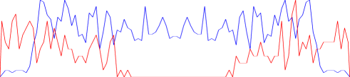
Figure 2: Probability distributions. Blue line is $\left(\frac{\displaystyle P_{1}}{\displaystyle 2}+\frac{\displaystyle P_{2}}{\displaystyle 2}\right)$, red line is $P_{12}$.

Let us denote the probability distribution in the first experiment (only upper slit is opened) as $P_{1}=P_{1}(y)$, in the the second experiment (only lower slit is opened) as $P_{2}=P_{2}(y)$, and in the third experiment (both slits are opened) as $P_{12}=P_{12}(y)$. Although since the force is different in each experiment, see (3), it is quite clear that (Fig.2)

$$P_{12}\neq\frac{P_{1}}{2}+\frac{P_{2}}{2}$$ (10)

To become an equality the above equation should have an extra term

$$P_{12}=\frac{P_{1}}{2}+\frac{P_{2}}{2}+\sqrt{P_{1}P_{2}}\cos\theta$$ (11)

where $\sqrt{P_{1}P_{2}}\cos\theta$ is a so-called interference term (Fig.3), and $\theta=\theta(y)$ is spread along $y$-axis.

Figure 3: Interference term, $\cos\theta=(2P_{12}-(P_{1}+P_{2}))/\sqrt{P_{1}P_{2}}$.

The function

$$\cos\theta=\frac{2P_{12}-(P_{1}+P_{2})}{\sqrt{P_{1}P_{2}}}$$ (12)

is shown on the (Fig.2). Please note that as there are ranges where $P_{1}$ or $P_{2}$ are equal to zero, i.e. $P_{1}P_{2}=0$ the function $\cos\theta$ is not determined and from (11) we see that $P_{12}$ does not depend on it.

Conclusion. We have shown that the proposed classical model has a context dependence and could be adequately described with contextual formalism. Quantum like behavior for macro systems is demonstrated. We simulate quantum-like interference for macroscopic objects. Such a simulation essentially reduced the gap between micro and macro worlds.

One of the authors (A.K.) would like to thank S. Albeverio, L. Accardy, L. Ballentine, V. Belavkin, E. Beltrametti, G. Cassinelli, A. Chebotarev, W. De Baere, W. De Myunck, R. Gill, D. Greenberger, S. Goldstein, C. Fuchs, L. Hardy, A. Holevo, T. Hida, P. Lahti, E. Loubents, D. Mermin, T. Maudlin, A. Peres, I. Pitowsky, A. Plotnitsky, A. Shiryaev, O. Smoljanov, J. Summhammer, L. Vaidman and I. Volovich, A. Zeilinger for fruitful discussions on probabilistic foundations of quantum mechanics.

This work was done during the visit of Ya.V. to Växjö University, he is grateful for the kind hospitality.

References

[1] P. A. M. Dirac, The Principles of Quantum Mechanics (Oxford Univ. Press, 1930).

[2] W. Heisenberg, Physical principles of quantum theory. (Chicago Univ. Press, 1930).

[3] N. Bohr, Phys. Rev., 48, 696-702 (1935).

[4] J. von Neumann, Mathematical foundations of quantum mechanics (Princeton Univ. Press, Princeton, N.J., 1955).

[5] R. Feynman and A. Hibbs, Quantum Mechanics and Path Integrals (McGraw-Hill, New-York, 1965).

[6] J. M. Jauch, Foundations of Quantum Mechanics (Addison-Wesley, Reading, Mass., 1968).

[7] P. Busch, M. Grabowski, P. Lahti, Operational Quantum Physics (Springer Verlag, 1995).

[8] B. d’Espagnat, Veiled Reality. An anlysis of present-day quantum mechanical concepts (Addison-Wesley, 1995).

[9] A. Peres, Quantum Theory: Concepts and Methods (Kluwer Academic Publishers, 1994).

[10] E. Beltrametti and G. Cassinelli, The logic of Quantum mechanics. (Addison-Wesley, Reading, Mass., 1981).

[11] L. E. Ballentine, Quantum mechanics (Englewood Cliffs, New Jersey, 1989).

[12] A.Yu. Khrennikov, Interpretations of probability (VSP Int. Publ., Utrecht, 1999).

[13] S. P. Gudder, J. Math Phys., 25, 2397 (1984); S. P. Gudder, N. Zanghi, Nuovo Cimento B 79, 291(1984).

[14] L. Accardi, Phys. Rep., 77, 169(1981); L. Accardi, in Stochastic processes in quantum theory and statistical physics, edited by S. Albeverio et al., Springer LNP 173 1 (1982). L. Accardi, Urne e Camaleoni: Dialogo sulla realta, le leggi del caso e la teoria quantistica. Il Saggiatore, Rome (1997). L.Accardi, P. Regoli: Quantum probability versus non-locality: crucial experiment. Preprint, Centro V. Volterra, N. 409, 2000.

[15] I. Pitowsky, Phys. Rev. Lett, 48, N.10, 1299(1982).

[16] A. Fine, Phys. Rev. Letters, 48, 291 (1982); P. Rastal, Found. Phys., 13, 555 (1983).

[17] W. De Baere, Lett. Nuovo Cimento, 39, 234 (1984); 25, 2397(1984); W. De Muynck, W. De Baere, H. Martens, Found. of Physics, 24, 1589 (1994);

[18] L. Ballentine, Probability theory in quantum mechanics. American J. of Physics, 54, 883-888 (1986).

[19] J. Summhammer, Int. J. Theor. Physics, 33, 171 (1994); Found. Phys. Lett. 1, 113 (1988); Phys.Lett., A136, 183 (1989).

[20] A. Yu. Khrennikov, Ensemble fluctuations and the origin of quantum probabilistic rule. Rep. MSI, Växjö Univ., 90, October (2000).

[21] A. Yu. Khrennikov, Classification of transformations of probabilities for preparation procedures: trigonometric and hyperbolic behaviours. Preprint quant-ph/0012141, 24 Dec 2000.

[22] A. Yu. Khrennikov, Linear representations of probabilistic transformations induced by context transitions. Preprint quant-ph/0105059, 13 May 2001.

[23] A. Yu. Khrennikov, ‘Quantum probabilities’ as context depending probabilities. Preprint quant-ph/0106073, 13 June 2001.

[24] A. Zeilinger, Recent results in fullerene Inteferometry and in quantum teleportation. Abstracts of Int. Conf. Exploring Quantum Physics, Venice-2001.

[25] A. Ben-Kish, J. Britton, D. Kielpinski, D. Leibfried, V. Meyer, M. Rowe, C. Sakket, W. Itano, C. Monroe, D. Wineland, Ion entanglement experiments at NIST-Boulder. Abstracts of Int. Conf. Exploring Quantum Physics, Venice-2001.