Field quantization for chaotic resonators with overlapping modes

Abstract

Feshbach’s projector technique is employed to quantize the electromagnetic field in optical resonators with an arbitrary number of escape channels. We find spectrally overlapping resonator modes coupled due to the damping and noise inflicted by the external radiation field. For wave chaotic resonators the mode dynamics is determined by a non–Hermitean random matrix. Upon including an amplifying medium, our dynamics of open-resonator modes may serve as a starting point for a quantum theory of random lasing.

Several recent experiments [2] have demonstrated laser action in amplifying random media. The experiments use highly disordered dielectrics in which light undergoes multiple chaotic scattering. The scattering can make light stay long enough inside the material for light amplification to become efficient. A random laser is created when the amplification rate exceeds the loss rate due to escape from the medium.

Theoretically, much is known [3] about the sub–threshold radiation from random lasers but only a few results exist in the non–linear lasing regime. Progress in this regime has been hampered by the unusual properties of the random laser modes. First, the mode amplitudes and mode frequencies in random lasers depend on the statistical properties of the underlying random medium. Random laser modes therefore must be analyzed in a statistical fashion, quite in contrast to traditional laser resonators. Moreover, the character of the modes depends on the amount of disorder. For strong disorder, localization of light may set in and give rise to well separated modes centered in different regions of space. By contrast, weak disorder leads to a poor confinement of light and to strongly overlapping modes.

Standard laser theory [4, 5] only applies to quasi–discrete modes and cannot account for lasing in the presence of overlapping modes. Various quantization schemes have been proposed [6, 7, 8] to replace the quasi–discrete modes of standard theory by quasimodes or Fox–Li modes of “bad” resonators. Unfortunately, these schemes are not well suited for a quantum statistical description required for random lasers. Statistics naturally enters the random-scattering theory pioneered by Beenakker [3], but that approach is restricted to linear media and cannot describe lasers above the lasing threshold. So far, to our knowledge, there is no satisfactory scheme for the field quantization in random media.

In the present paper we develop such a quantization scheme for optical resonators with overlapping modes. The resonator may have an irregular shape or may contain weak random scatterers to ensure chaotic scattering of light inside the cavity. We employ a technique previously applied to condensed matter physics, the Feshbach projector formalism. Using that method we show that the electromagnetic field Hamiltonian of open resonators reduces to the well–known system–and–bath Hamiltonian of quantum optics. Chaotic scattering enters that Hamiltonian in two ways. First, the frequency spectrum of the resonator modes shows the correlations and “level repulsion” typical for wave chaos. Second, the resonator mode amplitudes are not damped separately but coupled by dissipation. Both effects are related to the spectral properties of non–Hermitean random matrices and must eventually be included in a quantum theory of random lasing.

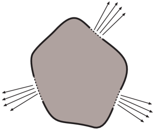
FIG. 1.: Sketch of a chaotic resonator that is connected to the external radiation field via a number of openings.

We start with the general solution of the quantization problem, and then discuss the application to chaotic scattering. For the sake of simplicity we consider a two dimensional optical resonator and TM fields; the polarization vector of the electric field defines the $z$–axis while ${\bf r}=(x,y)$ labels the position in the plane. The extension to three dimensional resonators and fields with arbitrary polarization will be given elsewhere [9]. Several openings make for a coupling to the external radiation field. The total width ${\cal W}$ of the openings determines the number $M$ of open escape channels at frequency $\omega$, $M\approx 2{\cal W}/\lambda$ with $\lambda=2\pi c/\omega$. The resonator modes near frequency $\omega$ are broadened over a frequency range $M\Delta\omega/2\pi$, much greater than their spacing $\Delta\omega$ if $M\gg 1$. The resonator boundary may have an arbitrary irregular shape. For simplicity we assume all walls perfectly conducting. The source free Maxwell equations reduce to the scalar wave equation

$$\left[\nabla^{2}-{1\over c^{2}}{\partial^{2}\over\partial t^{2}}\right]{A}({\bf r},t)=0$$ (1)

for the $z$–component $A({\bf r},t)$ of the vector potential. An exact quantum description of the total system comprising the resonator and the external radiation field is obtained by the so–called modes–of–the–universe approach [10, 11]. One expands both the vector potential ${A}$ and the canonical momentum field ${\Pi}\equiv\dot{A}/c^{2}$ in terms of the exact eigenmodes $\psi_{m}(\omega,{\bf r})$ of the Helmholtz equation

$$\left[\nabla^{2}+{\omega^{2}\over c^{2}}\right]\psi_{m}(\omega,{\bf r})=0.$$ (2)

They are labeled by the continuous frequency $\omega$ and the integer $m$; the latter specifies the asymptotic conditions far away from the resonator. For example, these conditions could correspond to a scattering problem with incoming and outgoing waves. Then $\psi_{m}(\omega,{\bf r})$ represents a solution with an incoming wave in channel $m$ and only outgoing waves in all other scattering channels. The channel index $m$ may correspond to an angular momentum quantum number (for a resonator coupled to free space) or to a transverse mode index (for resonators connected to external waveguides). It is convenient to combine the solutions associated with the different channels to an $M$–component vector $\psi(\omega,{\bf r})$. Then the field expansions take the form

$${A}({\bf r},t) = c\int\!d\omega\ q(\omega,t)\psi(\omega,{\bf r}),$$ (3)

$${\Pi}({\bf r},t) = {1\over c}\int\!d\omega\ \psi^{\dagger}(\omega,{\bf r})p(\omega,t),$$ (4)

where the operators $q(\omega)$ and $p(\omega)$ form $M$–component row and column vectors, respectively. Canonical commutation relation for $A({\bf r})$ and $\Pi({\bf r})$ follow by imposing the canonical commutation relations $[q_{m}(\omega),p_{n}(\omega^{\prime})]=i\hbar\delta_{mn}\delta(\omega-\omega^{\prime})$. The Hamiltonian of the problem is given by

$$H={1\over 2}\int d{\bf r}\left[c^{2}{\bf\Pi}({\bf r},t)^{2}+[\nabla\times{\bf A}({\bf r},t)]^{2}\right],$$ (5)

with ${\bf A}=A{\bf e}_{z}$ and ${\bf\Pi}=\Pi{\bf e}_{z}$. The Heisenberg equations of motion for ${\bf\Pi}$ and $\nabla\times{\bf A}$ are easily seen to reduce to the Maxwell equations.

The modes–of–the–universe approach yields a consistent quantization scheme, but does not provide any information about the resonator itself. In particular, no definition is obtained for the resonator modes, and a statistical description of these modes cannot be implemented at this point. However, further progress is possible since the Helmholtz equation with frequency $\omega$ is equivalent to a single–particle Schrödinger equation with energy $E=\omega^{2}/c^{2}$. That link between optics and single-particle quantum mechanics allows us to compute the mode functions $\psi(\omega,{\bf r})$ and to define resonator modes.

The calculation is performed using Feshbach’s projector formalism [12, 13]. The single–particle Hilbert space is decomposed into two orthogonal subspaces associated with the resonator and the channel region, respectively. The quantum Hamiltonian reads

$${\cal H} = \sum_{\lambda}E_{\lambda}|\phi_{\lambda}\rangle\langle\phi_{\lambda}|+\sum_{m}\int dEE|\chi_{m}(E)\rangle\langle\chi_{m}(E)|$$ (7)

$$+\sum_{\lambda m}\int\!\!dE\ \big{[}W_{\lambda m}(E)|\phi_{\lambda}\rangle\langle\chi_{m}(E)|+{\rm h.c.}\big{]}\,,$$

with the first two terms describing the decoupled resonator and waveguide, while the last term accounts for their coupling. We have chosen a basis in which both the resonator and the channel Hamiltonian are diagonal. We note that the Hamiltonian (7) is an exact representation of the eigenvalue problem (2), even in the regime of overlapping resonances.

The Hamiltonian (7) has been extensively used in the theory of chaotic scattering [13]. We employ the formulation appropriate for scattering through cavities. The resonator wave functions $\phi_{\lambda}({\bf r})$ are nonzero only within the resonator, while the channel wave functions $\chi(E,{\bf r})$ “live” only outside. We require that these functions obey Dirichlet conditions along the boundary of the total system (solid line in Fig. 1). The boundary condition along the surface separating the resonator from the waveguide (dashed line in Fig. 1) is arbitrary save that the total Hamiltonian be self-adjoint. The coupling amplitudes $W_{\lambda m}(E)$ are given by surface integrals involving appropriate resonator and channel wave functions.

Diagonalization of the Hamiltonian (7) yields the scattering states $\psi_{m}(E,{\bf r})$ with incoming wave in channel $m$ only. The modes functions are found from the mapping to the Helmholtz equation, $\psi(\omega,{\bf r})\equiv[\sqrt{2\omega}/c]\psi(E,{\bf r})$. They can be expressed as linear combinations of resonator and channel modes

$$\psi(\omega,{\bf r})=\sum_{\lambda}\alpha_{\lambda}(\omega)\phi_{\lambda}({\bf r})+\int d\omega^{\prime}\,\beta(\omega,\omega^{\prime})\chi(\omega^{\prime},{\bf r}),$$ (8)

with an $M$–component coefficient $\alpha_{\lambda}(\omega)$ and an $M\times M$ coefficient matrix $\beta(\omega,\omega^{\prime})$. Explicit expressions [13] for these coefficients are not needed below. Substituting Eq. (8) into Eqs. (4), one obtains the field expansions

$${A}({\bf r},t) = c\sum_{\lambda}Q_{\lambda}\phi_{\lambda}({\bf r})+c\int\!d\omega^{\prime}\,Q(\omega^{\prime})\chi(\omega^{\prime},{\bf r}),$$ (9)

$${\Pi}({\bf r},t) = {1\over c}\sum_{\lambda}\phi^{*}_{\lambda}({\bf r})P_{\lambda}+{1\over c}\int\!d\omega^{\prime}\,\chi^{\dagger}(\omega^{\prime},{\bf r})P(\omega^{\prime}),$$ (10)

where we have defined the position operators

$$Q_{\lambda}=\!\int\!d\omega\,q(\omega)\alpha_{\lambda}(\omega),\quad Q(\omega^{\prime})=\!\int\!d\omega\,q(\omega)\beta(\omega,\omega^{\prime}),$$ (11)

and the momentum operators

$$P_{\lambda}=\!\int\!d\omega\,\alpha^{\dagger}_{\lambda}(\omega)p(\omega),\quad P(\omega^{\prime})=\!\int\!d\omega\,\beta^{\dagger}(\omega,\omega^{\prime})p(\omega).$$ (12)

The final step of the quantization procedure is to express these operators in terms of photon creation and annihilation operators. For the resonator modes this is achieved by the representation

$$Q_{\lambda} = \left[{\hbar\over 2\omega_{\lambda}}\right]^{1/2}\,\big{[}a_{\lambda}+\sum_{\lambda^{\prime}}U^{\dagger}_{\lambda\lambda^{\prime}}a^{\dagger}_{\lambda^{\prime}}\big{]},$$ (13)

$$P_{\lambda} = i\left[\frac{\hbar\omega_{\lambda}}{2}\right]^{1/2}\,\big{[}a^{\dagger}_{\lambda}-\sum_{\lambda^{\prime}}U_{\lambda\lambda^{\prime}}a_{\lambda^{\prime}}\big{]},$$ (14)

where the matrix $U$ with the matrix elements

$$U_{\lambda\lambda^{\prime}}=\int d{\bf r}\phi_{\lambda}({\bf r})\phi_{\lambda^{\prime}}({\bf r})$$ (15)

specifies the spatial overlap of different resonator modes. We note that $U$ is unitary and symmetric, and that it only couples degenerate modes, $U_{\lambda\lambda^{\prime}}\sim\delta(\omega_{\lambda}-\omega_{\lambda^{\prime}})$, as modes with different frequencies have zero overlap (the modes are solutions of an Hermitean eigenvalue problem). The representation (13) realizes the commutation relations and, at the same time, secures Hermiticity for the intra–cavity fields, $A=A^{\dagger}$, $\Pi=\Pi^{\dagger}$. A similar representation is obtained for the channel modes with the replacements $a_{\lambda}\to b(\omega)$ and $U_{\lambda\lambda^{\prime}}\to U(\omega\omega^{\prime})$.

Substituting the representation (14) into the field expansions (10) and using the unitarity of $U$, we find the representation of the intra–cavity fields

$$A({\bf r},t) = c\sum_{\lambda}\left[{\hbar\over 2\omega_{\lambda}}\right]^{1/2}\,[a_{\lambda}\phi_{\lambda}({\bf r})+a_{\lambda}^{\dagger}\phi^{*}_{\lambda}({\bf r})],$$ (16)

$$E({\bf r},t) = i\sum_{\lambda}\left[{\hbar\omega_{\lambda}\over 2}\right]^{1/2}\,[a_{\lambda}\phi_{\lambda}({\bf r})-a_{\lambda}^{\dagger}\phi^{*}_{\lambda}({\bf r})].$$ (17)

Substitution of the field expansions into Eq. (5) finally yields the field Hamiltonian

$$H =\sum_{\lambda}\hbar\omega_{\lambda}a^{\dagger}_{\lambda}a_{\lambda}+\hbar\sum_{m}\int\!d\omega\,\omega b^{\dagger}_{m}(\omega)b_{m}(\omega)$$ (19)

$$+\hbar\sum_{\lambda m}\int\!\!d\omega\,W_{\lambda m}(\omega)\left[a^{\dagger}_{\lambda}b_{m}(\omega)+a^{\dagger}_{\lambda}b_{m}^{\dagger}(\omega)+h.c.\right],$$

where we defined $W_{\lambda m}(\omega)=[c/\hbar\sqrt{2\omega_{\lambda}}]W_{\lambda m}(E)$ and omitted an irrelevant constant on the right hand side. The equations (16) and (19) are the key results of the quantization procedure. The field expansions of the open resonator reduce precisely to the standard expressions known from closed resonators. However, the field dynamics is fundamentally different as shown below. We note that the resonator modes are coupled to the external radiation field via both resonant ($a^{\dagger}b$, $ab^{\dagger}$) and non–resonant ($ab$, $a^{\dagger}b^{\dagger}$) terms. The non-resonant terms can be discarded here since we are not interested in overdamping (where mode widths would be larger than or at least comparable to the optical frequencies). Our case of interest, the case of overlapping resonances, is fully compatible with the rotating–wave approximation, where only the resonant terms are kept. Then, the Hamiltonian (19) reduces to the well–known system–and–bath Hamiltonian [14] of quantum optics. It has been argued, that this Hamiltonian is valid only for good cavities with spectrally well–separated modes. Our derivation shows that such pessimism is inappropriate: the system–and–bath Hamiltonian does describe the dynamics of overlapping modes, provided the broadening of these modes is much smaller than their frequency (so that non–resonant terms can be neglected).

We now discuss the field dynamics and address the consequences of chaotic scattering. As a first example, we establish equations for the mode amplitudes. From the Hamiltonian (19) we obtain

$$\dot{a}_{\lambda}(t)=-i\omega_{\lambda}a_{\lambda}(t)-\!\pi\!\sum_{\lambda^{\prime}}(WW^{\dagger})_{\lambda\lambda^{\prime}}a_{\lambda^{\prime}}(t)+F_{\lambda}(t),$$ (20)

where $F_{\lambda}(t)$ is the noise operator

$$F_{\lambda}(t)=\int_{-\infty}^{\infty}d\omega e^{-i\omega(t-t_{0})}\sum_{m}W_{\lambda m}b_{m}(\omega,t_{0}),$$ (21)

and $W$ the coupling matrix with the elements $W_{\lambda m}$. The equations (20) differ drastically from the independent–oscillator equations of standard laser theory, in two respects: First, the mode operators $a_{\lambda}$ are coupled by the damping matrix $WW^{\dagger}$; second, the noise operators $F_{\lambda}$ are correlated, $\langle F^{\dagger}_{\lambda}F_{\lambda^{\prime}}\rangle\neq\delta_{\lambda\lambda^{\prime}}$, as different modes couple to the same external channels (the expectation value is defined with respect to the channel oscillators at time $t_{0}$).

A limiting case of Eq. (20) is the weak damping regime where all matrix elements of $WW^{\dagger}$ are much smaller than the resonator mode spacing $\Delta\omega$. This regime can be realized either by an opening smaller than a wavelength or by the insertion in the openings of partially reflecting mirrors. To leading order in $WW^{\dagger}/\Delta\omega$ only diagonal elements contribute to the damping matrix, and Eq. (20) reduces to the standard equation of motion for non–overlapping modes [4].

For the interesting case of wave chaos the internal Hamiltonian can be represented by a random matrix from the Gaussian orthogonal ensemble of random-matrix theory. The eigenvalues $\omega_{\lambda}$ display level repulsion and universal statistical properties. From Eq. (20), the mode dynamics of open chaotic resonators is governed by a non–Hermitean random matrix; we thus encounter an interesting connection between the spectral properties of open chaotic optical resonators and non–Hermitean random matrices [16].

As a second application of our field dynamics we now study an open resonator above the laser threshold. We focus on a single laser–line and compute the laser linewidth. The active medium is represented by ${\cal N}$ two–level atoms. To simplify the calculation, we assume (i) ${\cal N}\gg 1$ and spatially uniform gain , (ii) atomic decay rates that much exceed the field decay rates, (iii) exact resonance between the laser frequency $\bar{\omega}$ and the atomic transition frequency, and (iv) laser operation sufficiently far above threshold so that the field fluctuations can be obtained by linearization. The Heisenberg equations for the field mode amplitudes and the atomic polarization and inversion take the standard form [4] except for the mode coupling inflicted by damping and noise. We decompose the field into its classical steady–state value and the quantum fluctuations, $a_{\lambda}=(\bar{a}_{\lambda}+\delta a_{\lambda})\exp(-i\bar{\omega}t)$. The steady–state conditions take the form $0={\cal H}\cdot\bar{a}$ where $\bar{a}$ is an $N$–component vector comprising the steady–state amplitudes $\bar{a}_{\lambda}$ (the limit $N\to\infty$ is taken at the end of the calculation). The non–Hermitean matrix

$${\cal H}_{\lambda\lambda^{\prime}}=(\omega_{\lambda}-\bar{\omega})\delta_{\lambda\lambda^{\prime}}-\pi(WW^{\dagger})_{\lambda\lambda^{\prime}}+G\delta_{\lambda\lambda^{\prime}},$$ (22)

depends on the laser field intensity $I=\sum_{\lambda}|\bar{a}_{\lambda}|^{2}$ via the gain $G=(2S{\cal N}g^{2}/\gamma_{\perp})(1+4g^{2}I/\gamma_{\parallel}\gamma_{\perp})^{-1}$. Here, $S$ denotes the pumping strength, $g$ is the atom–field coupling, and $\gamma_{\perp}$ and $\gamma_{\parallel}$ are the decay rates for the atomic polarization and population inversion. The equations of motion for the quantum fluctuations follow upon linearization around the steady–state solution

$$\left(\begin{array}[]{c}\delta\dot{a}\\ \delta\dot{a}^{\dagger}\end{array}\right)={\cal L}\left(\begin{array}[]{c}\delta a\\ \delta a^{\dagger}\end{array}\right)+\left(\begin{array}[]{c}{\cal F}\\ {\cal F}^{\dagger}\end{array}\right).$$ (23)

The noise operators ${\cal F}$, ${\cal F}^{\dagger}$ incorporate both field noise and noise from the atomic reservoirs. The dynamics of $\delta a$ and $\delta a^{\dagger}$ is coupled by the $2N\times 2N$ matrix

$${\cal L}=\left(\begin{array}[]{cc}-i{\cal H}&0\\ 0&i{\cal H}^{*}\end{array}\right)+\frac{\partial G}{\partial I}\left(\begin{array}[]{cc}\bar{a}\cdot\bar{a}^{\dagger}&\bar{a}\cdot\bar{a}^{T}\\ \bar{a}^{*}\cdot\bar{a}^{\dagger}&\bar{a}^{*}\cdot\bar{a}^{T}\end{array}\right)$$ (24)

which depends explicitly on the steady–state solution $\bar{a}$. Equations (23), (24) reduce the computation of the field fluctuations to the spectral decomposition of the non–Hermitean matrix ${\cal L}$. One easily shows that ${\cal L}$ has a zero eigenvalue connected with the well-known process of phase diffusion. The corresponding right eigenvector has the form $(r,-r^{*})$, where $r\propto\bar{a}$ is a right eigenvector to eigenvalue $0$ of the $N\times N$ matrix ${\cal H}$; the existence of $r$ and the corresponding left eigenvector $l$ is guaranteed by the steady–state equations, $0={\cal H}\cdot\bar{a}$. The phase–diffusion coefficient and the laser linewidth $\delta\omega$ can now be computed along standard lines [4, 5]: We solve the equations of motion (23) and calculate the Fourier transform of the stationary correlator $\langle\delta a^{\dagger}(t)\delta a(0)\rangle$. Keeping only the zero–eigenvalue contribution in the spectral decomposition of ${\cal L}$, we obtain the linewidth

$$\delta\omega=K\delta\omega_{\rm ST},$$ (25)

which is larger than the fundamental (Schawlow–Townes) linewidth $\delta\omega_{\rm ST}$ by the Petermann factor [17, 18]

$$K=\langle l|l\rangle\langle r|r\rangle.$$ (26)

The non–zero eigenvalues of ${\cal L}$ will generally modify the Lorentzian spectrum and the laser lineshape [19]. A detailed investigation of these modifications, their statistics in a random medium, the pertinent photon statistics [20], as well as the generalization to multi–mode lasing will be published separately.

Support by the Sonderforschungsbereich “Unordnung und große Fluktuationen” der Deutschen Forschungsgemeinschaft is gratefully acknowledged.

REFERENCES

- [1]
- [2] H. Cao et al., Phys. Rev. Lett. 82, 2278 (1999); H. Cao et al., Phys. Rev. Lett. 84, 5584 (2000); H. Cao et al., Phys. Rev. Lett. 86, 4524 (2001).
- [3] C. W. J. Beenakker, Phys. Rev. Lett. 81, 1829 (1998).
- [4] H. Haken, Laser theory, 2nd edition (Springer, Berlin, 1984); Light (North–Holland, Amsterdam, 1985).
- [5] M. Sargent III, M. O. Scully, and W. E. Lamb, Laser Physics (Addison Wesley, Reading, MA, 1974).
- [6] B. J. Dalton, S. M. Barnett, and P. L. Knight, J. Mod. Opt. 46, 1315 (1999).
- [7] C. Lamprecht and H. Ritsch, Phys. Rev. Lett. 82, 3787 (1999).
- [8] S. M. Dutra and G. Nienhuis, Phys. Rev. A 62, 063805 (2000).
- [9] C. Viviescas and G. Hackenbroich, quant-ph/0203122.
- [10] R. Lang, M. O. Scully, and W. E. Lamb, Phys. Rev. A 7, 1788 (1973).
- [11] R. J. Glauber and M. Lewenstein, Phys. Rev. A 43, 467 (1991).
- [12] H. Feshbach, Ann. Phys. (N.Y.) 19, 287 (1962).
- [13] F. M. Dittes, Phys. Rep. 339, 216 (2000).
- [14] C. W. Gardiner and P. Zoller, Quantum Noise, 2nd edition (Springer, Berlin, 2000).
- [15] F. Haake, Quantum Signatures of Chaos, 2nd edition (Springer, Berlin, 2000).
- [16] Y. V. Fyodorov and H.–J. Sommers, J. Math. Phys. 38, 1918 (1997); J. T. Chalker and B. Mehlig, Phys. Rev. Lett. 81, 3367 (1998).
- [17] K. Petermann, IEEE J. Quantum Electron. 15, 566 (1979).
- [18] A. E. Siegman, Phys. Rev. A 39, 1253 (1989); Phys. Rev. A 39, 1264 (1989).
- [19] S. M. Dutra et al., Phys. Rev. A 59, 4699 (1999).
- [20] G. Hackenbroich, C. Viviescas, B. Elattari, and F. Haake, Phys. Rev. Lett. 86, 5262 (2001).