Phase-transition-like Behavior of Quantum Games

Abstract

The discontinuous dependence of the properties of a quantum game on its entanglement has been shown up to be very much like phase transitions viewed in the entanglement-payoff diagram [J. Du et al., Phys. Rev. Lett, 88, 137902 (2002)]. In this paper we investigate such phase-transition-like behavior of quantum games, by suggesting a method which would help to illuminate the origin of such kind of behavior. For the particular case of the generalized Prisoners’ Dilemma, we find that, for different settings of the numerical values in the payoff table, even though the classical game behaves the same, the quantum game exhibits different and interesting phase-transition-like behavior.

1 Introduction

The theory of quantum games is a new born field which combines the classical game theory and the quantum information theory, opening a new range of potential applications. Recent research have shown that quantum games can outperform their classical counterparts [1, 2, 3, 4, 5, 6, 7, 8, 9, 10, 11]. J. Eisert et al. investigated the quantization of the famous game of Prisoners’ Dilemma [4]. Their result exhibits the surprising superiority of quantum strategies over classical ones and the players can escape the dilemma when they both resort to quantum strategies. L. Marinatto and T. Weber studied the quantum version of the Battle of the Sexes game and found that the game can have a unique solution with entangled strategy [5]. Besides two player quantum games, works on multiplayer games have also been presented [6, 7]. In a recent paper of S.C. Benjamin and P.M. Hayden, they showed that multiplayer quantum games can exhibit certain forms of pure quantum equilibrium that have no analogue in classical games, or even in two player quantum games [6]. Although most of the works are focused on maximally entangled quantum games, game of varying entanglement is also investigated [9, 10]. For the particular case of the two-player quantum Prisoners’ Dilemma, two thresholds for the game’s entanglement is found, and the phenomena which are very much like phase transitions are also revealed. Even though quantum game are played mostly on paper, the first experimental realization of quantum games has also been implemented on a NMR quantum computer [11].

In this paper, we investigate the phase-transition-like behavior of quantum games, using a proposed method which would help to illuminate the origin of such kind of behavior. For the generalized version of Prisoners’ Dilemma, we find that, with different settings of the numerical values for the payoff table, even though the classical game behaves the same, the quantum game behaves greatly differently and exhibits interesting phase-transition-like behavior in the entanglement-payoff diagram. We find thresholds for the amount of entanglement that separate different regions for the game. The properties of the game changes discontinuously when its entanglement goes across these thresholds, creating the phase-transition-like behavior. We present investigation for both the case where the strategic space is restricted as in Ref. [4] and the case where the players are allowed to adopt any unitary operations as their strategies. In the case where the strategic space is restricted, the phase-transition-like behavior exhibits interesting variation with respect to the change of the numerical values in the payoff table, so does the property of the game. In the case where the players are allowed to adopt any unitary operations, the game has an boundary, being a function of the numerical values in the payoff table, for its entanglement. The quantum game has an infinite number of Nash equilibria if its entanglement is below the boundary, otherwise no pure strategic Nash equilibrium could be found when its entanglement exceeds the boundary.

The proposed method would help to illuminate the origin of such kind of phase-transition-like behavior. In this method, strategies of players are corresponding to unit vectors in some real space, and the searching for Nash equilibria includes a procedure of finding the eigenvector of some matrix that corresponds to the maximal eigenvalue. In the particular case presented in this paper, the eigenvalues are functions of the amount of entanglement, and thus there can be an eigenvalue-crossing. Crossing an eigenvalue-crossing point makes the eigenvector that corresponds to the maximal eigenvalue changes discontinuously, indicating the discontinuous change of the properties of the quantum game, as well as the phase-transition-like behavior.

2 Quantization of The Generalized Prisoners’ Dilemma

Table 1: The general form of the Prisoners’ Dilemma. The first entry in the parenthesis denotes the payoff of Alice and the second number the payoff of Bob. The entries in this table should satisfy conditions: $t>r>p>s$ (see in Reference [12]). The meanings of the symbols in the table is as follows. $C$: Cooperate; $D$: Defect; $r$: reward; $p$: punishment; $t$: temptation; $s$: sucker’s payoff.

• 	Bob: $C$	Bob: $D$
  Alice: $C$	$\left(r,r\right)$	$\left(s,t\right)$
  Alice: $D$	$\left(t,s\right)$	$\left(p,p\right)$

The classical Prisoners’ Dilemma is the most widely studied and used paradigm as a non-zero-sum game that could have an equilibrium outcome which is unique, but fails to be Pareto optimal. The importance of this game lies in the fact that many social phenomena with which we are familiar seem to have Prisoner’s Dilemma at their core. The general form of the Prisoners’ Dilemma [12] is shown as in Table 1, with suggestive names for the strategies and payoffs. The condition $t>r>p>s$ guarantees that strategy $D$ dominates strategy $C$ for both players, and that the unique equilibrium at $\left(D,D\right)$ is Pareto inferior to $\left(C,C\right)$.

• 

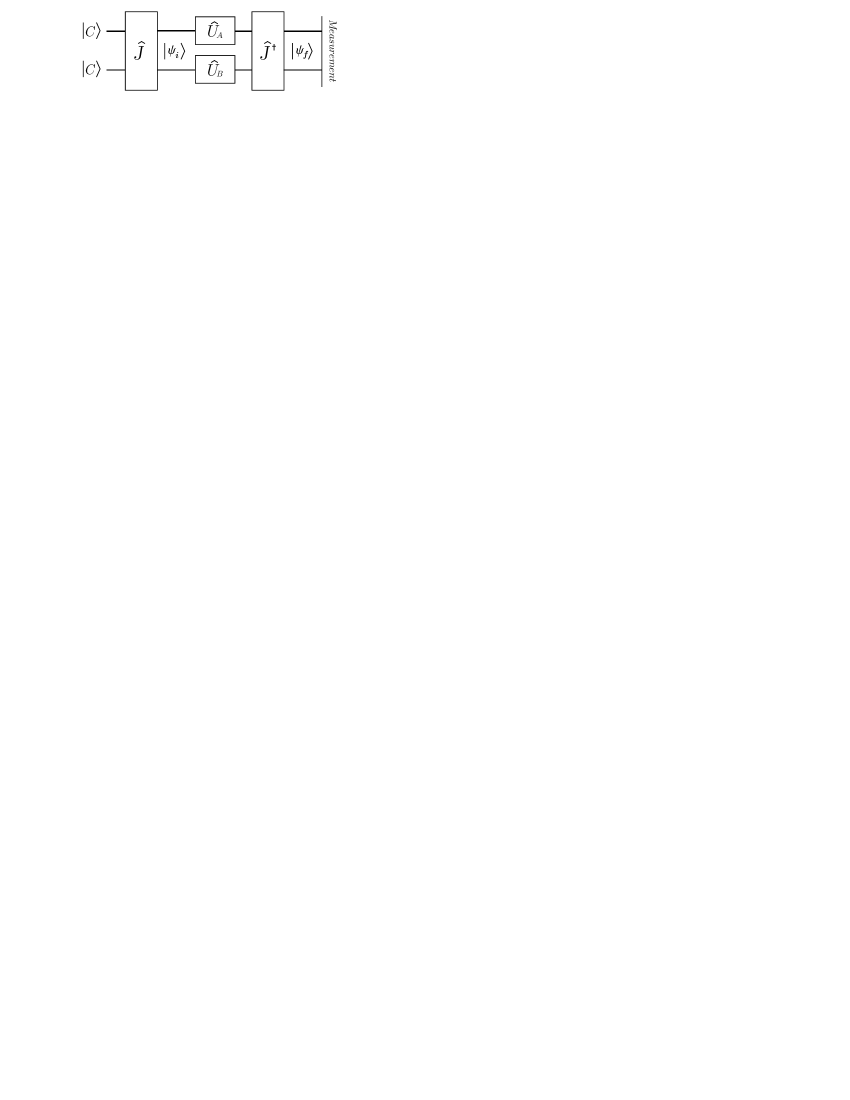
Figure 1: The physical model for two player quantum Prisoners’ Dilemma.

The physical model of the quantum Prisoners’ Dilemma is originally proposed by J. Eisert et al. as shown in Fig. 1. Together with the payoff table for the general Prisoners’ Dilemma, the scheme can represent the generalized quantum Prisoners’ Dilemma. In this scheme the game has two qubits, one for each player. The possible outcomes of the classical strategies $D$ and $C$ are assigned to two basis $\left|D\right\rangle$ and $\left|C\right\rangle$ in the Hilbert space of a qubit. Hence the state of the game at each instance is described by a vector in the tensor product space which is spanned by the classical game basis $\left|CC\right\rangle$, $\left|CD\right\rangle$, $\left|DC\right\rangle$ and $\left|DD\right\rangle$, where the first and second entries refer to Alice’s and Bob’s qubits respectively. The initial state of the game is given by

$$\left|\psi_{i}\right\rangle=\hat{J}\left|CC\right\rangle,$$ (1)

where $\hat{J}$ is a unitary operator which is known to both players. Strategic moves of Alice and Bob are associated with unitary operators $\hat{U}_{A}$ and $\hat{U}_{B}$ respectively, which are chosen from a strategic space $S$. At the final stage, the state of the game is

$$\left|\psi_{f}\right\rangle=\hat{J}^{{\dagger}}\left(\hat{U}_{A}\otimes\hat{U}_{B}\right)\hat{J}\left|CC\right\rangle.$$ (2)

The subsequent measurement yields a particular result and the expect payoffs of the players are given by

$$\left\{\begin{array}[c]{c}\$_{A}=rP_{CC}+pP_{DD}+tP_{DC}+sP_{CD}\\ \$_{B}=rP_{CC}+pP_{DD}+sP_{DC}+tP_{CD}\end{array}\right.,$$ (3)

where $P_{\sigma\tau}=\left|\left\langle\sigma\tau\right|\left.\psi_{f}\right\rangle\right|^{2}$ $\left(\sigma,\tau\in\left\{C,D\right\}\right)$ is the probability that $\left|\psi_{f}\right\rangle$ collapses into basis $\left|\sigma\tau\right\rangle$.

In the general case, strategies for players could be any unitary operations. However, since the overall phase factor of $\left|\psi_{f}\right\rangle$ will not affect the final results of the game, we can safely set the strategic space $S=SU\left(2\right)$ as in Refs. [4] and [6], without loss of generality.

As we known, an operator $\hat{U}\in SU\left(2\right)$ can be written as

$$\hat{U}=w\cdot\hat{I}_{2}+x\cdot i\hat{\sigma}_{x}+y\cdot i\hat{\sigma}_{y}+z\cdot i\hat{\sigma}_{z},$$ (4)

with $w,x,y,z\in\left[-1,1\right]$ and $w^{2}+x^{2}+y^{2}+z^{2}=1$. This enables us to represent $\hat{U}$ directly by a four-dimensional real vector

$$u=\left(w,x,y,z\right)\in\mathbb{R}^{4},$$ (5)

with $u\cdot u^{T}=w^{2}+x^{2}+y^{2}+z^{2}=1$ (superscript $T$ denotes Transpose), and its components are denoted as $u^{1}=w,u^{2}=x,u^{3}=y,u^{4}=z$.

Denote Alice’s strategy by $u_{A}$ and Bob’s by $u_{B}$, the payoffs in Eq. (3) can be written as

$$\left\{\begin{array}[c]{c}\$_{A}=\$_{A}\left(u_{A},u_{B}\right)=\sum_{ij,kl}\$_{ij,kl}^{A}\cdot u_{A}^{i}u_{A}^{j}u_{B}^{k}u_{B}^{l}\\ \$_{B}=\$_{B}\left(u_{A},u_{B}\right)=\sum_{ij,kl}\$_{ij,kl}^{B}\cdot u_{B}^{i}u_{B}^{j}u_{A}^{k}u_{A}^{l}\end{array}\right.,$$ (6)

where $i,j,k,l$ run from $1$ to $4$, $\left(\$_{ij,kl}^{A}\right)$ and $\left(\$_{ij,kl}^{B}\right)$ are certain tensors. The formulation of $\left(\$_{ij,kl}^{A}\right)$ and $\left(\$_{ij,kl}^{B}\right)$ in Eq. (6) are not uniquely determined. However if restricted to be symmetric, i.e. $\$_{ij,kl}^{A}=\$_{ji,kl}^{A}=\$_{ij,lk}^{A}$ and $\$_{ij,kl}^{B}=\$_{ji,kl}^{B}=\$_{ij,lk}^{B}$ (this can always be done), they both can be uniquely determined. The calculations for $\left(\$_{ij,kl}^{A}\right)$ and $\left(\$_{ij,kl}^{B}\right)$ could be found in A. Eqs. (6) are actually very general formulations for any static quantum game expressed as in Table 1 and Fig. 1 (the gate $\hat{J}^{{\dagger}}$ prior to measurement can even be replaced by other unitary transformation, not necessarily the inverse of $\hat{J}$). All the structural information of the game, including the classical payoff table and the physical model, is represented by the tensors $\left(\$_{ij,kl}^{A}\right)$ and $\left(\$_{ij,kl}^{B}\right)$. In the Prisoners’ Dilemma, we have $\$_{ij,kl}^{A}\equiv\$_{ij,kl}^{B}$ due to the symmetric structure of the game. In an asymmetric game, $\left(\$_{ij,kl}^{A}\right)$ does not necessarily equals $\left(\$_{ij,kl}^{B}\right)$.

Defining $\$_{ij,kl}\equiv\$_{ij,kl}^{A}\equiv\$_{ij,kl}^{B}$, Eq. (6) can be re-expressed as

$$\left\{\begin{array}[c]{c}\$_{A}\left(u_{A},u_{B}\right)=\sum_{ij}\left(\sum_{kl}\$_{ij,kl}\cdot u_{B}^{k}u_{B}^{l}\right)u_{A}^{i}u_{A}^{j}=u_{A}\cdot P\left(u_{B}\right)\cdot u_{A}^{T}\\ \$_{B}\left(u_{A},u_{B}\right)=\sum_{ij}\left(\sum_{kl}\$_{ij,kl}\cdot u_{A}^{k}u_{A}^{l}\right)u_{B}^{i}u_{B}^{j}=u_{B}\cdot P\left(u_{A}\right)\cdot u_{B}^{T}\end{array}\right.,$$ (7)

where $P\left(u\right)$ is a symmetric matrix as a function of $u$, whose $i,j$-th element satisfies

$$\left(P\left(u\right)\right)_{ij}=\sum_{kl}\$_{ij,kl}\cdot u^{k}u^{l}.$$ (8)

Let $\left(u_{A}^{\ast},u_{B}^{\ast}\right)$ be a Nash equilibrium of the game, we can see that, from Eq. (7), $u_{A}\cdot P\left(u_{B}^{\ast}\right)\cdot u_{A}^{T}$ reaches its maximum at $u_{A}=u_{A}^{\ast}$ and simultaneously $u_{B}\cdot P\left(u_{A}^{\ast}\right)\cdot u_{B}^{T}$ reaches its maximum at $u_{B}=u_{B}^{\ast}$. In terms of game theory, we say that $u_{A}^{\ast}$ dominates $u_{B}^{\ast}$ and $u_{B}^{\ast}$ dominates $u_{A}^{\ast}$. Together with $u_{A}^{\ast}\cdot\left(u_{A}^{\ast}\right)^{T}=u_{B}^{\ast}\cdot\left(u_{B}^{\ast}\right)^{T}=1$, we can conclude that $u_{A}^{\ast}$ ($u_{B}^{\ast}$) must be the eigenvector of $P\left(u_{B}^{\ast}\right)$ [$P\left(u_{A}^{\ast}\right)$] which corresponds to the maximal eigenvalue, and the corresponding eigenvalue is exactly the payoff for Alice (Bob) at this Nash equilibrium. This analysis also tells that the dominant strategy against a given strategy $u$ must be the eigenvector of $P\left(u\right)$ that corresponds to the maximal eigenvalue.

In the following, we will first investigate the general Prisoners’ Dilemma in the case that the strategic space is restricted to be the 2-parameter subset of $SU\left(2\right)$ as given in Ref. [4]. Then we investigate this game when the players are allowed to adopt any unitary strategic operations. Here we shall note that some authors [15] have argued that the restriction on the strategic space given in Ref. [4] has no physical basis, and it does restrict generality. However, apart from these arguments, it is still an interesting case and a good instance to show how the phase-transition-like behavior originates. Yet the particular results achieved hold only for this very specific set of strategies.

3 Two-Parameter Set of Strategies

In the case of two-parameter set of strategies, the strategic space $S$ is restricted to the two-parameter subset of $SU\left(2\right)$ as follows [4],

$$\hat{U}\left(\theta,\varphi\right)=\left(\begin{array}[c]{cc}e^{i\varphi}\cos\theta/2&\sin\theta/2\\ -\sin\theta/2&e^{-i\varphi}\cos\theta/2\end{array}\right),$$ (9)

with $\theta\in\left[0,\pi\right]$ and $\varphi\in\left[0,\pi/2\right]$.

As illustrated in details by J. Eisert et al. [4], in order to guarantee that the classical Prisoners’ Dilemma is faithfully represented, the form of $\hat{J}$ should be

$$\hat{J}=e^{i\gamma\hat{D}\otimes\hat{D}/2}=\cos\frac{\gamma}{2}\hat{C}\otimes\hat{C}+i\sin\frac{\gamma}{2}\hat{D}\otimes\hat{D},$$ (10)

where $\hat{C}=$ $\hat{U}\left(0,0\right)$, $\hat{D}=\hat{U}\left(\pi,0\right)$, and $\gamma\in\left[0,\pi/2\right]$ is in fact a measure for the game’s entanglement.

Eq. (9) can be rewritten as

$$\hat{U}\left(\theta,\varphi\right) =\cos\frac{\theta}{2}\cos\varphi\cdot\hat{I}_{2}+\sin\frac{\theta}{2}\cdot i\hat{\sigma}_{y}+\cos\frac{\theta}{2}\sin\varphi\cdot i\hat{\sigma}_{z}$$ (11)

$$=w\cdot\hat{I}_{2}+y\cdot i\hat{\sigma}_{y}+z\cdot i\hat{\sigma}_{z},$$

where $w=\cos\frac{\theta}{2}\cos\varphi,y=\sin\frac{\theta}{2},z=\cos\frac{\theta}{2}\sin\varphi$. Obviously we have $w,y,z\in\left[0,1\right]$ and $\hat{U}\left(\theta,\varphi\right)\in SU\left(2\right)$ implies that $w^{2}+y^{2}+z^{2}=1$. Since $\hat{U}\left(\theta,\varphi\right)$ and $-\hat{U}\left(\theta,\varphi\right)$ represent the same strategy, it is enough to restrict ourselves with $w,y,z\in\left[-1,1\right]$. Therefore in the case of two-parameter set of strategies, $\hat{U}\left(\theta,\varphi\right)$ can be represented by a three-dimensional real vector

$$u=\left(w,y,z\right)\in\mathbb{R}^{3},$$ (12)

with $u\cdot u^{T}=w^{2}+y^{2}+z^{2}=1$. Eqs. (6, 7, 8) will remain their form, except that all the indices run only from $1$ to $3$, rather than from $1$ to $4$. Obviously we have $\hat{C}\sim\left(1,0,0\right),\hat{D}\sim\left(0,1,0\right),\hat{Q}\sim\left(0,0,1\right)$, in which “$\sim$” means “represent (by)”. In the remaining part of this paper, we do not distinguish a unitary operator and the corresponding vector (3-dimensional or 4-dimensional), as long as there is not ambiguity.

In Ref. [9], we investigated this game in the case that $\left(r,p,t,s\right)=\left(3,1,5,0\right)$ and observed the phenomenon that are very much like phase transitions. In the generalized quantum Prisoners’ Dilemma, such phase-transition-like behavior still exists. In fact, there exist two thresholds for the game’s entanglement, $\gamma_{th1}=\arcsin\sqrt{\left(p-s\right)/\left(t-s\right)}$ and $\gamma_{th2}=\arcsin\sqrt{\left(t-r\right)/\left(t-s\right)}$. We hereby prove that, for $0\leqslant\gamma<\gamma_{th1}$, the strategic profile $\hat{D}\otimes\hat{D}$ is the Nash equilibrium with payoffs $\$_{A}=\$_{B}=p$. For $\gamma_{th2}<\gamma\leqslant\pi/2$, the strategic profile $\hat{Q}\otimes\hat{Q}$ is the Nash equilibrium with payoffs $\$_{A}=\$_{B}=r$. If $\gamma_{th1}<\gamma_{th2}$ and $\gamma_{th1}\leqslant\gamma\leqslant\gamma_{th2}$, the game has two Nash equilibria $\hat{D}\otimes\hat{Q}$ and $\hat{Q}\otimes\hat{D}$. The payoff for the player who adopts $\hat{D}$ is $s+\left(t-s\right)\cos^{2}\gamma$ while for the player who adopts $\hat{Q}$ is $s+\left(t-s\right)\sin{}^{2}\gamma$. While if $\gamma_{th2}<\gamma_{th1}$ and $\gamma_{th2}\leqslant\gamma\leqslant\gamma_{th1}$, both $\hat{D}\otimes\hat{D}$ and $\hat{Q}\otimes\hat{Q}$ are Nash equilibria of the game. We obtain these conclusions through the following steps:

Assume one player adopts strategy $\hat{D}$, the payoff for the other as the function of his/her strategy $u$ is

$$u\cdot P\left(\hat{D}\right)\cdot u^{T},$$ (13)

where the explicit expression of $P\left(\hat{D}\right)$ is (the calculation could be found in B)

$$P\left(\hat{D}\right)=\left(\begin{array}[c]{ccc}s&0&0\\ 0&p&0\\ 0&0&s+\left(t-s\right)\sin{}^{2}\gamma\end{array}\right).$$ (14)

If $0\leqslant\gamma<\gamma_{th1}=\arcsin\sqrt{\left(p-s\right)/\left(t-s\right)}$, the maximal eigenvalue of $P\left(\hat{D}\right)$ is $p$, and the corresponding eigenvector is $\left(0,1,0\right)\sim\hat{D}$. If $\gamma_{th1}<\gamma\leqslant\pi/2$, the maximal eigenvalue of $P\left(\hat{D}\right)$ is $s+\left(t-s\right)\sin{}^{2}\gamma$, and the corresponding eigenvector is $\left(0,0,1\right)\sim\hat{Q}$. Therefore $\hat{D}$ dominates $\hat{D}$ for $0\leqslant\gamma<\gamma_{th1}$ while $\hat{Q}$ dominates $\hat{D}$ for $\gamma_{th1}<\gamma\leqslant\pi/2$. For the same time we have $\$_{A}\left(\hat{D},\hat{D}\right)=\$_{B}\left(\hat{D},\hat{D}\right)=p$ and $\$_{A}\left(\hat{Q},\hat{D}\right)=\$_{B}\left(\hat{D},\hat{Q}\right)=s+\left(t-s\right)\sin{}^{2}\gamma$.

While assume one player adopts strategy $\hat{Q}$, the payoff for the other as the function of his/her strategy $u$ is

$$u\cdot P\left(\hat{Q}\right)\cdot u^{T},$$ (15)

where the explicit expression of $P\left(\hat{Q}\right)$ is (the calculation could be found in B)

$$P\left(\hat{Q}\right)=\left(\begin{array}[c]{ccc}r-\left(r-p\right)\sin{}^{2}\gamma&0&0\\ 0&t-\left(t-s\right)\sin{}^{2}\gamma&0\\ 0&0&r\end{array}\right).$$ (16)

If $0\leqslant\gamma<\gamma_{th2}=\arcsin\sqrt{\left(t-r\right)/\left(t-s\right)}$, the maximal eigenvalue of $P\left(\hat{Q}\right)$ is $t-\left(t-s\right)\sin{}^{2}\gamma$, and the corresponding eigenvector is $\left(0,1,0\right)\sim\hat{D}$. If $\gamma_{th2}<\gamma\leqslant\pi/2$, the maximal eigenvalue of $P\left(\hat{Q}\right)$ is $r$, and the corresponding eigenvector is $\left(0,0,1\right)\sim\hat{Q}$. Therefore $\hat{D}$ dominates $\hat{Q}$ for $0\leqslant\gamma<\gamma_{th2}$ while $\hat{Q}$ dominates $\hat{Q}$ for $\gamma_{th2}<\gamma\leqslant\pi/2$. For the same time we have $\$_{A}\left(\hat{Q},\hat{Q}\right)=\$_{B}\left(\hat{Q},\hat{Q}\right)=r$ and $\$_{A}\left(\hat{D},\hat{Q}\right)=\$_{B}\left(\hat{Q},\hat{D}\right)=t-\left(t-s\right)\sin{}^{2}\gamma=s+\left(t-s\right)\cos^{2}\gamma$.

From the above analysis, we can see that when $0\leqslant\gamma<\gamma_{th1}$, $\hat{D}\otimes\hat{D}$ is a Nash equilibrium of the game, and when $\gamma_{th2}<\gamma\leqslant\pi/2$, $\hat{Q}\otimes\hat{Q}$ is a Nash equilibrium of the game. If $\gamma_{th1}<\gamma_{th2}$ and $\gamma_{th1}\leqslant\gamma\leqslant\gamma_{th2}$, $\hat{D}$ dominates $\hat{Q}$ and $\hat{Q}$ dominates $\hat{D}$, hence both $\hat{D}\otimes\hat{Q}$ and  $\hat{Q}\otimes\hat{D}$ are Nash equilibria of the game. While if $\gamma_{th2}<\gamma_{th1}$ and $\gamma_{th2}\leqslant\gamma\leqslant\gamma_{th1}$, both $\hat{D}\otimes\hat{D}$ and $\hat{Q}\otimes\hat{Q}$ are Nash equilibria of the game. The corresponding payoffs are also obtained.

• 

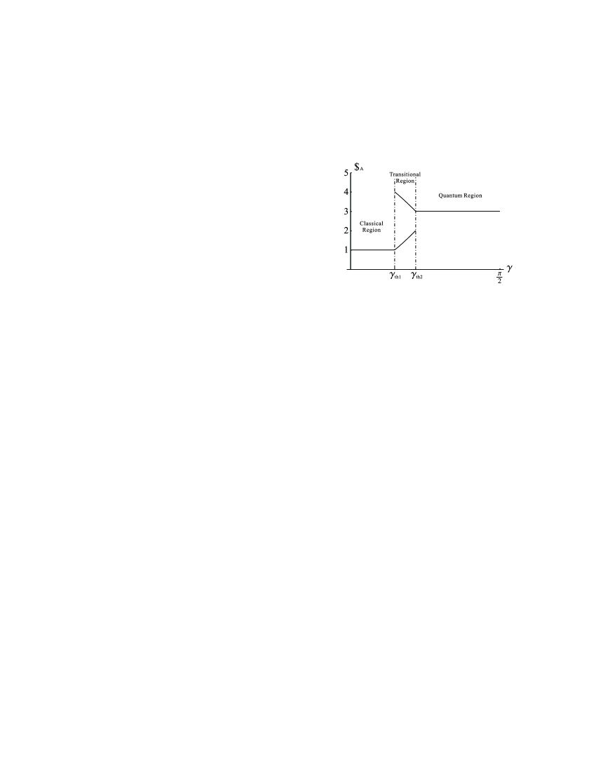
Figure 2: The payoff function of Alice with respect to the amount of the entanglement in the case of two-parameter strategies. The numerical values in the payoff matrix are set as $(r=3,p=1,t=5,s=0)$ such that $r+p<t+s$. The region between two thresholds are the transitional region from classical to quantum, in which the game has two asymmetric Nash equilibria although the game is symmetric with respect to the interchange of the players.

In the case that the entries in the payoff table are taken as $\left(r=3,p=1,t=5,s=0\right)$, which has been investigated in Ref[9], the game has two thresholds for the amount of the game’s entanglement. Due to the two thresholds, the game is divided into three regions, the classical region, the quantum region, and the transitional region from classical to quantum. In the general quantum Prisoners’ Dilemma, there still exist two thresholds and the phase-transition-like behavior shows up again. However the situation may be more complicated because the two thresholds have no deterministic relations in magnitude. In fact, the case that $\left(r=3,p=1,t=5,s=0\right)$ is just an instance of the more general case of $r+p<t+s$. For the game under this condition, it is obviously that $\gamma_{th1}<\gamma_{th2}$ and the game behaves similarly to the one with $\left(r=3,p=1,t=5,s=0\right)$. Fig. 2 depicts the payoff of Alice as the function of $\gamma$ when both players resort to Nash equilibrium in the case of $r+p<t+s$. In the transitional regions, the two Nash equilibria are fully equivalent. Since there is no communication between two players, one player will have no idea which equilibrium strategy the other player chooses. So the strategy mismatch situation will probably occur. A more severe problem is that, since strategy $\hat{D}$ will lead to a better payoff so both players will be tempted to choose $\hat{D}$ and the final payoff for both of them will become $p$, which happens to be the catch of the dilemma in the classical game.

An interesting situation is, as we can see, if $\gamma_{th1}=\gamma_{th2}$, the transitional region will disappear. The condition $\gamma_{th1}=\gamma_{th2}$ implies that

$$r+p=t+s.$$ (17)

Note that we should keep in mind that the basic condition $t>r>p>s$ must be satisfied to maintain the properties of the classical game. And under the condition in Eq. (17) the game has only one threshold for its entanglement $\gamma_{th}=\gamma_{th1}=\gamma_{th2}$. Hence the game exhibits only two regions, one is classical and the other is quantum. The transitional region in which the game has two asymmetric Nash equilibrium disappears. Under the conditions $r+p=t+s$ and $t>r>p>s$, we plot the payoff of Alice as the function of $\gamma$ in Fig. 3 when both players resort to Nash equilibrium.

• 

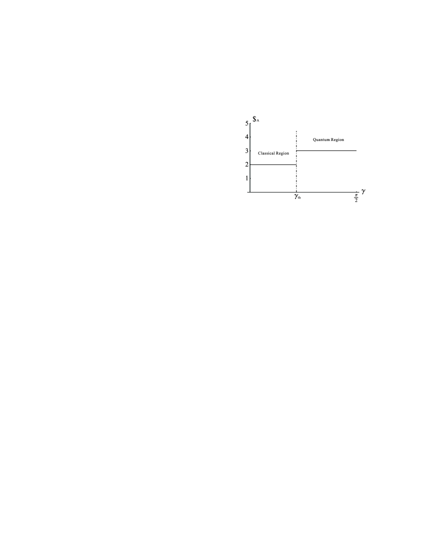
Figure 3: The payoff function of Alice with respect to the amount of the entanglement in the case of two-parameter strategies. The numerical values in the payoff matrix are set as $(r=3,p=2,t=5,s=0)$ such that $r+p=t+s$. The two thresholds converge to be a unique one $\gamma_{th}$ and the transitional region no longer exists.

Now we consider what would happen in the game of $r+p>t+s$. In this case, we have $\gamma_{th1}>\gamma_{th2}$. Therefore the game has no transitional region, hence none of $\hat{D}\otimes\hat{Q}$ and $\hat{Q}\otimes\hat{D}$ is a Nash equilibrium of the game. However both $\hat{D}\otimes\hat{D}$ and $\hat{Q}\otimes\hat{Q}$ are still Nash equilibria in the region $\gamma_{th2}\leqslant\gamma\leqslant\gamma_{th1}$. So for $\gamma_{th2}\leqslant\gamma\leqslant\gamma_{th1}$, a new region — coexistent region — arises with two Nash equilibria. These two Nash equilibria are both symmetric with respect to the interchange of the two players. In this case, we illustrate the payoff of Alice as the function of $\gamma$ in Fig. 4. We should also note that in this case the multiple Nash equilibria brings a situation different to that in the transitional regions with $r+p<t+s$. The two Nash equilibria are not equivalent and $\hat{Q}\otimes\hat{Q}$ gives higher payoffs to both players than does $\hat{D}\otimes\hat{D}$. Therefore it is a quite reasonable assumption that the players are most likely to resort to the equilibrium $\hat{Q}\otimes\hat{Q}$ rather than $\hat{D}\otimes\hat{D}$, since they are both trying to maximize their individual payoffs. However, one still can not claim that the players will definitely resort to the equilibrium that gives higher payoffs. But if they do, the final results of the game will then be the same as in the quantum region with $\gamma>\gamma_{th1}$, and the dilemma will be resolved.

An interesting question is that can the game behave full quantum-mechanically no matter how much it is entangled for some particular numerical value of $\left(r,p,t,s\right)$, i.e. have only the quantum region (without the presence of classical, transitional or coexistent regions). If it can, we immediately deduce that $\gamma_{th2}=0$. This means $t=r$, which contradicts the basic condition $t>r>p>s$. Hence the game cannot always have $\hat{Q}\otimes\hat{Q}$ as its equilibrium in the whole domain of $\gamma$ from $0$ to $\pi/2$, as long as the game remains a “Prisoners’ Dilemma”. In fact, as long as the condition $t>r>p>s$ holds, none of $\gamma_{th1}$ and $\gamma_{th2}$ could reach $0$ or $\pi/2$, hence none of the classical and quantum regions will disappear.

• 

Figure 4: The payoff function of Alice with respect to the amount of the entanglement in the case of two-parameter strategies. The numerical values in the payoff matrix are set as $(r=3,p=2,t=4,s=0)$ such that $r+p>t+s$. The coexistent region emerges, in which both $\hat{D}\otimes\hat{D}$ and $\hat{Q}\otimes\hat{Q}$ are Nash equilibria.

4 General Unitary Operations

In this section, we investigate the generalized quantum Prisoners’ Dilemma when both the players can access to any unitary operations as their strategies, rather than in a restricted subset in Eq. (9). The method for analyzing is clearly described in section 2. The result is that, there exist a boundary $\gamma_{B}=\arcsin\sqrt{\left(p-s\right)/\left(p+t-r-s\right)}$ for the game’s entanglement. If $\gamma<\gamma_{B}$, there are infinite Nash equilibrium. Any strategic profile $\left\{\left(0,\alpha,\beta,0\right),\left(0,\beta,\alpha,0\right)\right\}$ ($\alpha^{2}+\beta^{2}=1$) is a Nash equilibrium. Each of them results in the same payoffs $\$_{A}=\$_{B}=p+\left(r-p\right)\sin^{2}\gamma$. While as long as $\gamma>\gamma_{B}$, there will be no Nash equilibrium for the game. We prove these results as follows.

For the strategy $u_{1}=\left(0,\alpha,\beta,0\right)$ ($\alpha^{2}+\beta^{2}=1$), we have (the calculation could be found in A), with $\epsilon\equiv\sin^{2}\gamma$,

$$P\left(u_{1}\right)=\left(\begin{array}[c]{cccc}s+\left(t-s\right)\alpha^{2}\epsilon&0&0&\left(s-t\right)\alpha\beta\epsilon\\ 0&p+\left(r-p\right)\beta^{2}\epsilon&\left(r-p\right)\alpha\beta\epsilon&0\\ 0&\left(r-p\right)\alpha\beta\epsilon&p+\left(r-p\right)\alpha^{2}\epsilon&0\\ \left(s-t\right)\alpha\beta\epsilon&0&0&s+\left(t-s\right)\beta^{2}\epsilon\end{array}\right).$$ (18)

The eigenvalues and corresponding eigenvectors of $P\left(\left(0,\alpha,\beta,0\right)\right)$ in Eq. (18) are

$$\left\{\begin{array}[c]{ll}p&\quad\left(0,\alpha,-\beta,0\right)\\ s&\quad\left(\beta,0,0,\alpha\right)\\ p+\left(r-p\right)\sin^{2}\gamma&\quad\left(0,\beta,\alpha,0\right)\\ s+\left(t-s\right)\sin^{2}\gamma&\quad\left(\alpha,0,0,-\beta\right)\end{array}\right..$$ (19)

If $\gamma<\gamma_{B}$, the maximal eigenvalue is $p+\left(r-p\right)\sin^{2}\gamma$ and the corresponding eigenvector is $\left(0,\beta,\alpha,0\right)$. Therefore $\left(0,\beta,\alpha,0\right)$ dominates $\left(0,\alpha,\beta,0\right)$, and vice versa (by exchanging $\alpha$ and $\beta$ in Eqs. (18, 19)). Hence any strategic profile $\left\{\left(0,\alpha,\beta,0\right),\left(0,\beta,\alpha,0\right)\right\}$ ($\alpha^{2}+\beta^{2}=1$) is a Nash equilibrium.

While if $\gamma>\gamma_{B}$, the dominant strategy against $\left(0,\alpha,\beta,0\right)$ turns to be $\left(\alpha,0,0,-\beta\right)$. For the strategy $u_{2}=\left(\alpha,0,0,-\beta\right)$, we have (the calculation could be found in A), with $\epsilon\equiv\sin^{2}\gamma$,

$$P\left(u_{2}\right)=\left(\begin{array}[c]{cccc}r+\left(p-r\right)\beta^{2}\epsilon&0&0&\left(r-p\right)\alpha\beta\epsilon\\ 0&t+\left(s-t\right)\alpha^{2}\epsilon&\left(s-t\right)\alpha\beta\epsilon&0\\ 0&\left(s-t\right)\alpha\beta\epsilon&t+\left(s-t\right)\beta^{2}\epsilon&0\\ \left(r-p\right)\alpha\beta\epsilon&0&0&r+\left(p-r\right)\alpha^{2}\epsilon\end{array}\right).$$ (20)

And the eigenvalues and corresponding eigenvectors of $P\left(\left(\alpha,0,0,-\beta\right)\right)$ in Eq. (20) are

$$\left\{\begin{array}[c]{ll}r&\quad\left(\alpha,0,0,\beta\right)\\ t&\quad\left(0,\beta,-\alpha,0\right)\\ r+\left(p-r\right)\sin^{2}\gamma&\quad\left(\beta,0,0,-\alpha\right)\\ t+\left(s-t\right)\sin^{2}\gamma&\quad\left(0,\alpha,\beta,0\right)\end{array}\right..$$ (21)

In Eq. (21), $\left(0,\beta,-\alpha,0\right)$ always corresponds to the maximal eigenvalue $t$. Therefore no matter what the amount of entanglement is, $\left(0,\beta,-\alpha,0\right)$ always dominates $\left(\alpha,0,0,-\beta\right)$. With further analysis combining Eq. (19) and Eq. (21), we find that when $\gamma>\gamma_{B}$, $\left(\alpha,0,0,-\beta\right)$ dominates $\left(0,\alpha,\beta,0\right)$, $\left(0,\beta,-\alpha,0\right)$ dominates $\left(\alpha,0,0,-\beta\right)$, $\left(\beta,0,0,\alpha\right)$ dominates $\left(0,\beta,-\alpha,0\right)$, and finally $\left(0,\alpha,\beta,0\right)$ dominates $\left(\beta,0,0,\alpha\right)$. No pair of them can form a Nash equilibrium. In fact, it can be proved that no pair of strategies in the region of $\gamma>\gamma_{B}$ can form a pure Nash equilibrium of the game. However the game remains to have mixed Nash equilibria [14].

We depict the payoff function of Alice as a function of the amount of entanglement when both players resort to Nash equilibrium (if there is one) in Fig. 5. This figure also exhibits the phase-transition-like behavior of the game. The boundary of entanglement divides the game into two regions: in one of which the game has infinite Nash equilibria, while in the other the game has no pure strategic Nash equilibrium.

• 

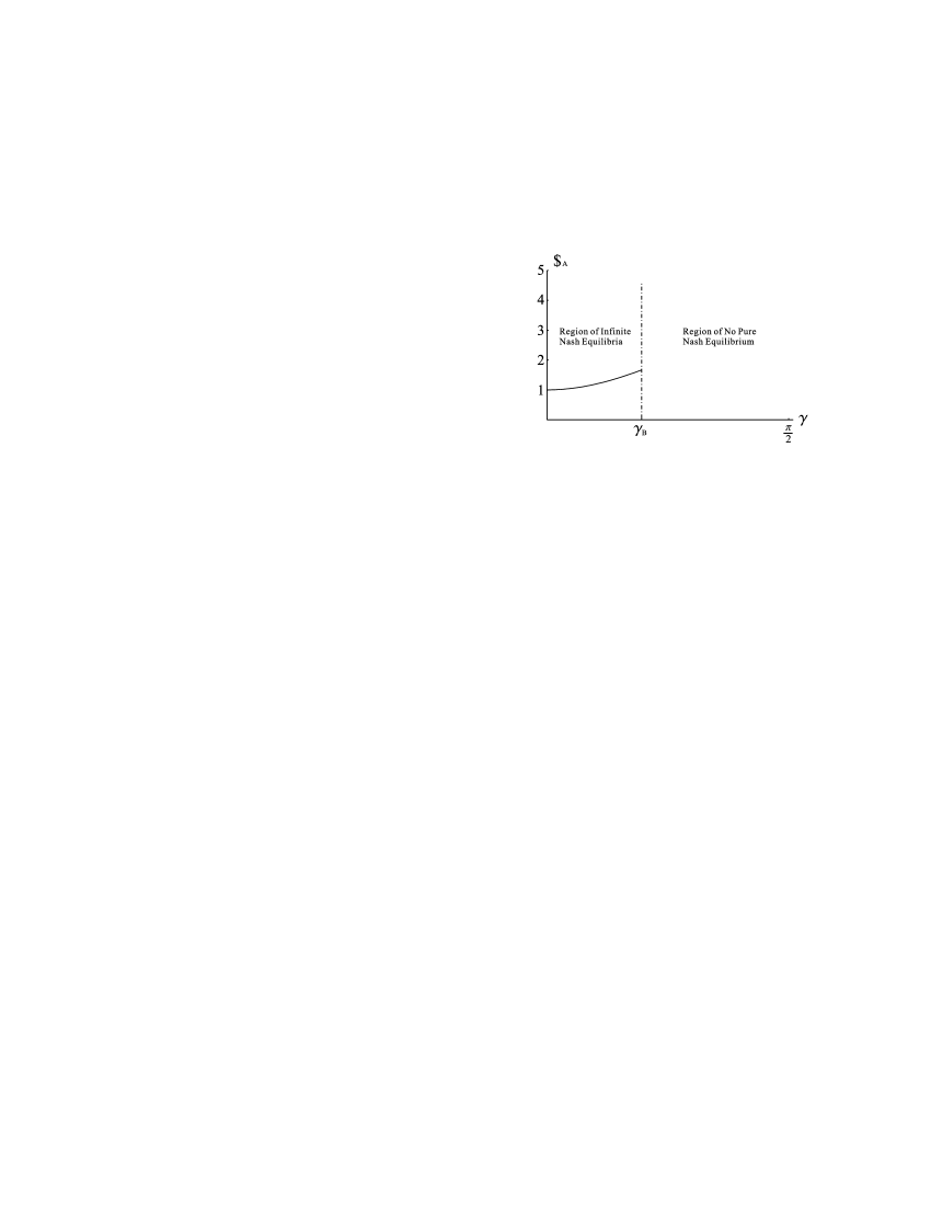
Figure 5: The payoff function of Alice with respect to the amount of the entanglement in the case that both players are allowed to adopt any unitary operator as his/her strategy.

5 Discussion and Conclusion

In this paper, we investigate the discontinuous dependence of Nash equilibria and payoffs on the game’s entanglement for the general quantum Prisoners’ Dilemma. This discontinuity can be viewed as the phase-transition-like behavior in the payoff-entanglement diagram. We firstly investigate the generalized quantum Prisoners’ Dilemma when the strategic space is restricted to be a two-parameter subset of $SU\left(2\right)$ as in Ref. [4]. With condition $r+p<t+s$, the game exhibits the classical, quantum and transitional regions in its payoff-entanglement diagram. The original Prisoners’ Dilemma with $\left(r=3,p=1,t=5,s=0\right)$ is just an instance for the general game with condition $r+p<t+s$. In the classical region $\hat{D}\otimes\hat{D}$ is the unique Nash equilibrium, and in the quantum region the unique Nash equilibrium is $\hat{Q}\otimes\hat{Q}$. While in the transitional region, two asymmetric Nash equilibria, $\hat{D}\otimes\hat{Q}$ and $\hat{Q}\otimes\hat{D}$, emerge, each leads to the asymmetric result of the game in despite of the symmetry of the game itself. If the entries in the payoff table satisfy that $r+p=t+s$, the transitional region will disappear. The game has only one threshold for the amount of its entanglement at which the game transits from classical to quantum discontinuously. In the case that $r+p>t+s$, a new region — the coexistent region — emerges, replacing the transitional region. This new region is in fact there where the classical region and the quantum region overlap. In the coexistent region, the game has both $\hat{D}\otimes\hat{D}$ and $\hat{Q}\otimes\hat{Q}$ as its Nash equilibria. Since $\hat{Q}\otimes\hat{Q}$ is superior to $\hat{D}\otimes\hat{D}$, one may expect both players most likely to choose $\hat{Q}$ as his/her strategy, and the dilemma will be resolved if they do so. We also explored the phase-transition-like behavior of the quantum game in the case where both players are allowed to adopt any unitary transformations as their strategies. The game has an boundary for its entanglement, being a function of the numerical values in the payoff table, below which the game has infinite Nash equilibria, while above which the game has no pure strategic Nash equilibrium.

The phase-transition-like behavior presented in this paper is very much like phase transitions in real physical systems [13], not only phenomenally but also mathematically. For a certain physical system whose Hamiltonian is dependent of some parameter, a special case is that the eigenfunctions of the Hamiltonian is independent of the parameter even though the eigenvalues vary with it. Then there can be a level-crossing where an excited level becomes the ground state, creating a point of a non-analyticity of the ground state energy as a function of the parameter, as well as a discontinuous dependence of the ground state on the parameter. A quantum phase transition is hence viewed as any point of non-analyticity in the ground state energy of the system concerned. In the generalized quantum Prisoners’ Dilemma, the dominant strategy against a given strategy $u$ is the eigenvector that corresponds to the maximal eigenvalue of matrix $P\left(u\right)$ (see in Section 2). Since $P\left(u\right)$ is a function of the amount of entanglement $\gamma$, the eigenvalues may cross. This eigenvalue-crossing makes the eigenvector that corresponds to the maximal eigenvalue changes discontinuously. It also creates a non-analyticity of the payoff (the maximal eigenvalue) as a function of $\gamma$, and the game exhibit phase-transition-like behavior. The method proposed in this paper would help to illuminate the origin of the phase-transition-like behavior of quantum games, and we hope it would further help investigate quantum games more intensively, and more profound results may be derived.

Appendix A Calculations For General Unitary Operations

Denote Alice’s strategy by $u_{A}=\left(u_{A}^{1},u_{A}^{2},u_{A}^{3},u_{A}^{4}\right)$ and Bob’s by $u_{B}=\left(u_{B}^{1},u_{B}^{2},u_{B}^{3},u_{B}^{4}\right)$, then substitute Eq. (4) into Eq. (2), we have

$$\left|\psi_{f}\right\rangle= [\left(u_{A}^{1}u_{B}^{1}-u_{A}^{4}u_{B}^{4}\right)+i\left(u_{A}^{4}u_{B}^{1}+u_{A}^{1}u_{B}^{4}\right)\cos\gamma-\left(u_{A}^{3}u_{B}^{2}+u_{A}^{2}u_{B}^{3}\right)\sin\gamma]\left|CC\right\rangle+$$ (22)

$$[-\left(u_{A}^{1}u_{B}^{3}+u_{A}^{4}u_{B}^{2}\right)+i\left(u_{A}^{1}u_{B}^{2}-u_{A}^{4}u_{B}^{3}\right)\cos\gamma+\left(u_{A}^{3}u_{B}^{4}-u_{A}^{2}u_{B}^{1}\right)\sin\gamma]\left|CD\right\rangle+$$

$$[-\left(u_{A}^{3}u_{B}^{1}+u_{A}^{2}u_{B}^{4}\right)+i\left(u_{A}^{2}u_{B}^{1}-u_{A}^{3}u_{B}^{4}\right)\cos\gamma+\left(u_{A}^{4}u_{B}^{3}-u_{A}^{1}u_{B}^{2}\right)\sin\gamma]\left|DC\right\rangle+$$

$$[\left(u_{A}^{3}u_{B}^{3}-u_{A}^{2}u_{B}^{2}\right)-i\left(u_{A}^{3}u_{B}^{2}+u_{A}^{2}u_{B}^{3}\right)\cos\gamma+\left(u_{A}^{4}u_{B}^{1}+u_{A}^{1}u_{B}^{4}\right)\sin\gamma]\left|DD\right\rangle.$$

Since the game is symmetric with respect to the interchange of the players, we have

$$\$_{A}\left(u_{A},u_{B}\right)\equiv\$_{B}\left(u_{B},u_{A}\right),\forall u_{A},u_{B}\in SU\left(2\right).$$ (23)

and we can immediately see from Eq. (6) that

$$\$_{ij,kl}^{A}\equiv\$_{ij,kl}^{B},i,j=1,2,3,4.$$ (24)

And $P\left(u\right)$ (in Eq. (8)) is symmetric too. Therefore we can define $\$_{ij,kl}\equiv\$_{ij,kl}^{A}\equiv\$_{ij,kl}^{B}$ for convenience. Substitute Eq. (22) into Eqs. (3, 6), we can find the non-zero elements of $\left(\$_{ij,kl}\right)$ are (with $\$_{ij,kl}=\$_{ji,kl}=\$_{ij,lk}=\$_{ji,lk}$)

$$\$_{11,11} =\$_{44,44}=r,\$_{11,33}=\$_{44,22}=s,$$

$$\$_{22,22} =\$_{33,33}=p,\$_{22,44}=\$_{33,11}=t,$$

$$\$_{11,22} =\$_{44,33}=s+\left(t-s\right)\sin^{2}\gamma,\$_{11,44}=\$_{44,11}=r+\left(p-r\right)\sin^{2}\gamma,$$

$$\$_{22,11} =\$_{33,44}=t+\left(s-t\right)\sin^{2}\gamma,\$_{22,33}=\$_{33,22}=p+\left(r-p\right)\sin^{2}\gamma,$$

$$\$_{12,13} =-\$_{34,24}=\frac{1}{2}\left(s-r\right)\sin\gamma,\$_{12,24}=-\$_{34,13}=\frac{1}{2}\left(t-p\right)\sin\gamma,$$

$$\$_{13,12} =-\$_{24,34}=\frac{1}{2}\left(t-r\right)\sin\gamma,\$_{13,34}=-\$_{24,12}=\frac{1}{2}\left(p-s\right)\sin\gamma,$$

$$\$_{14,14} =-\$_{23,23}=\frac{1}{2}\left(p-r\right)\sin^{2}\gamma,\$_{14,23}=-\$_{23,14}=\frac{1}{2}\left(s-t\right)\sin^{2}\gamma.$$ (25)

For strategy $\left(0,\alpha,\beta,0\right)$, we see that

$$\left(P\left(\left(0,\alpha,\beta,0\right)\right)\right)_{ij} =\left(P\left(\left(0,\alpha,\beta,0\right)\right)\right)_{ji}$$ (26)

$$=\alpha^{2}\$_{ij,22}+\beta^{2}\$_{ij,33}+\alpha\beta\left(\$_{ij,23}+\$_{ij,32}\right)$$

$$=\alpha^{2}\$_{ij,22}+\beta^{2}\$_{ij,33}+2\alpha\beta\$_{ij,23}$$

and for $\left(\alpha,0,0,-\beta\right)$ we have

$$\left(P\left(\left(\alpha,0,0,-\beta\right)\right)\right)_{ij} =\left(P\left(\left(\alpha,0,0,-\beta\right)\right)\right)_{ji}$$ (27)

$$=\alpha^{2}\$_{ij,11}+\beta^{2}\$_{ij,44}-\alpha\beta\left(\$_{ij,14}+\$_{ij,41}\right)$$

$$=\alpha^{2}\$_{ij,11}+\beta^{2}\$_{ij,44}-2\alpha\beta\$_{ij,14}.$$

Therefore Eq. (18) and (20) are obtained.

Appendix B Calculations For Two-Parameter Strategic Space

The two-parameter strategic space can be obtained by restricting $u^{2}=x\equiv 0$ in the general case ($u^{2}=x$ is the second component of $u$, not its squared length). Therefore the expressions for $\$_{ij,kl}$ can be obtained from Eqs. (25), by excluding all elements containing the index $2$, and then replacing index $3$ by $2$ and $4$ by $3$. Therefore for the case of two-parameter strategic space, we have all the non-zero elements (with $\$_{ij,kl}=\$_{ji,kl}=\$_{ij,lk}=\$_{ji,lk}$) as follows.

$$\$_{11,11} =\$_{33,33}=r,\$_{11,22}=s,\$_{22,22}=p,\$_{22,11}=t,$$

$$\$_{33,22} =s+\left(t-s\right)\sin^{2}\gamma,\$_{11,33}=\$_{33,11}=r+\left(p-r\right)\sin^{2}\gamma,$$

$$\$_{22,33} =t+\left(s-t\right)\sin^{2}\gamma,\$_{13,13}=\frac{1}{2}\left(p-r\right)\sin^{2}\gamma,$$

$$\$_{23,12} =\frac{1}{2}\left(p-t\right)\sin\gamma,\$_{12,23}=\frac{1}{2}\left(p-s\right)\sin\gamma.$$ (28)

Since $\hat{D}\sim\left(0,1,0\right)$ and $\hat{Q}\sim\left(0,0,1\right)$, it is obvious to see that

$$\left(P\left(\hat{D}\right)\right)_{ij} =\left(P\left(\hat{D}\right)\right)_{ji}=\$_{ij,22},$$ (29)

$$\left(P\left(\hat{Q}\right)\right)_{ij} =\left(P\left(\hat{Q}\right)\right)_{ji}=\$_{ij,33},$$ (30)

with $i,j=1,2,3$. The expressions in Eqs. (14) and (16) are hence obtained.

References

References

• [1] P. Ball, Nature Science Update, 18 Oct. 1999.
• [2] I. Peteron, Science News 156, 334 (1999).
• [3] G. Collins, Sci. Am. Jan. 2000.
• [4] J. Eisert et al., Phys. Rev. Lett. 83, 3077 (1999).
• [5] L. Marinatto and T. Weber. Phys. Lett. A 272. 291 (2000).
• [6] S.C. Benjamin and P.M. Hayden, Phys. Rev. A 64, 030301(R) (2001).
• [7] Jiangfeng Du et al., Phys. Lett. A 302, 229 (2002).
• [8] D.A. Meyer, Phys. Rev. Lett. 82, 1052 (1999).
• [9] Jiangfeng Du et al., Phys. Lett. A 289, 9 (2001).
• [10] A.P. Flitney and D. Abbott, quant-ph/0209121.
• [11] Jiangfeng Du et al., Phys. Rev. Lett. 88, 137902 (2002).
• [12] P.D. Straffin, Game Theory and Strategy (The Mathematical Association of America, 1993). The original general Prisoners’ Dilemma has an additional condition, $r>\left(s+t\right)/2$, besides $t>r>p>s$. This additional condition guarantees that even in an iterated game, the players would be at least as well off always playing $\left(C,C\right)$ as alternating between $\left(C,D\right)$ and $\left(D,C\right)$. So the strategy profile $\left(C,C\right)$ is Pareto optimal in both static and iterated game. In this paper we focus on the study of static games, so it is unnecessary for us to consider this additional condition.
• [13] S. Sachdev, Quantum Phase Transitions (Cambridge University Press, 1999).
• [14] J. Eisert and M. Wilkins, J. Mod. Opt. 47, 2543 (2000).
• [15] S.C. Benjamin and P.M. Hayden, Phys. Rev. Lett. 87, 069801 (2001).