Wannier-Stark resonances in optical and semiconductor superlattices

Abstract

Abstract:
In this work, we discuss the resonance states of a quantum particle in a periodic potential plus a static force. Originally this problem was formulated for a crystal electron subject to a static electric field and it is nowadays known as the Wannier-Stark problem. We describe a novel approach to the Wannier-Stark problem developed in recent years. This approach allows to compute the complex energy spectrum of a Wannier-Stark system as the poles of a rigorously constructed scattering matrix and solves the Wannier-Stark problem without any approximation. The suggested method is very efficient from the numerical point of view and has proven to be a powerful analytic tool for Wannier-Stark resonances appearing in different physical systems such as optical lattices or semiconductor superlattices.

PACS: 03.65.-w; 05.45.+b; 32.80.Pj; -73.20.Dx

Chapter 1 Introduction

The problem of a Bloch particle in the presence of additional external fields is as old as the quantum theory of solids. Nevertheless, the topics introduced in the early studies of the system, Bloch oscillations [1], Zener tunneling [2] and the Wannier-Stark ladder [3], are still the subject of current research. The literature on the field is vast and manifold, with different, sometimes unconnected lines of evolution. In this introduction we try to give a survey of the field, summarize the different theoretical approaches and discuss the experimental realizations of the system. It should be noted from the very beginning that most of the literature deals with one-dimensional single-particle descriptions of the system, which, however, capture the essential physics of real systems. Indeed, we will also work in this context.

1.1 Wannier-Stark problem

In the one-dimensional case the Hamiltonian of a Bloch particle in an additional external field, in the following referred to as the Wannier-Stark Hamiltonian, has the form

$$H_{W}=\frac{p^{2}}{2m}+V(x)+Fx,\quad V(x+d)=V(x),$$ (1.1)

where $F$ stands for the static force induced by the external field. Clearly, the external field destroys the translational symmetry of the field-free Hamiltonian $H_{0}=p^{2}/2m+V(x)$. Instead, from an arbitrary eigenstate with $H_{W}\Psi=E_{0}\Psi$, one can by a translation over $l$ periods $d$ construct a whole ladder of eigenstates with energies $E_{l}=E_{0}+ldF$, the so-called Wannier-Stark ladder. Any superposition of these states has an oscillatory evolution with the time period

$$T_{B}=\frac{2\pi\hbar}{dF}\;,$$ (1.2)

known as the Bloch period. There has been a long-standing controversy about the existence of the Wannier-Stark ladder and Bloch oscillations [4, 5, 6, 7, 8, 9, 10, 11, 12, 13, 14, 15, 16, 17, 18, 19], and only recently agreement about the nature of the Wannier-Stark ladder was reached. The history of this discussion is carefully summarized in [12, 20, 21, 22].

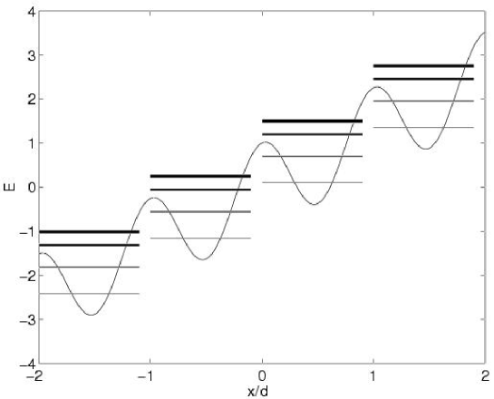
Figure 1.1: Schematic illustration of the Wannier-Stark ladder of resonances. The width of the levels is symbolized by the different strength of the lines.

From today’s point of view the discussion mainly dealt with the effect of the single band approximation (effectively a projection on a subspace of the Hilbert space) on the spectral properties of the Wannier-Stark Hamiltonian. Within the single band approximation, the $\alpha$’th band of the field-free Hamiltonian $H_{0}$ forms, if the field is applied, the Wannier-Stark ladder with the quantized energies

$$E_{\alpha,l}=\bar{\epsilon}_{\alpha}+dFl\;,\quad l=0\pm 1,\ldots\;,$$ (1.3)

where $\bar{\epsilon}_{\alpha}$ is the mean energy of the $\alpha$-th band (see Sec. 1.2). This Wannier-Stark quantization was the main point to be disputed in the discussions mentioned above. The process, which is neglected in the single band approximation and which couples the bands, is Zener tunneling [2]. For smooth potentials $V(x)$, the band gap decreases with increasing band index. Hence, as the tunneling rate increases with decreasing band gap, the Bloch particles asymmetrically tend to tunnel to higher bands and the band population depletes with time (see Sec. 1.3). This already gives a hint that Eq. (1.3) can be only an approximation to the actual spectrum of the sytem. Indeed, it has been proven that the spectrum of the Hamiltonian (1.1) is continuous [23, 24]. Thus the discrete spectrum (1.3) can refer only to resonances [25, 26, 27, 28, 29], and Eq. (1.3) should be corrected as

$$\mathcal{E}_{\alpha,l}=E_{\alpha}+dFl-{\rm i}\,\frac{\Gamma_{\alpha}}{2}\;,$$ (1.4)

(see Fig. 1.1). The eigenstates of the Hamiltonian (1.1) corresponding to these complex energies, referred in what follows as the Wannier-Stark states $\Psi_{\alpha,l}(x)$, are metastable states with the lifetime given by $\tau=\hbar/\Gamma_{\alpha}$. To find the complex spectrum (1.4) (and corresponding eigenstates) is an ultimate aim of the Wannier-Stark problem.

Several attempts have been made to calculate the Wannier-Stark ladder of resonances. Some analytical results have been obtained for nonlocal potentials [30, 31] and for potentials with a finite number of gaps [32, 33, 34, 35, 36, 37, 38]. (We note, however, that almost all periodic potentials have an infinite number of gaps.) A common numerical approach is the formalism of a transfer matrix to potentials which consist of piecewise constant or linear parts, eventually separated by delta function barriers [39, 40, 41, 42, 43]. Other methods approximate the periodic system by a finite one [44, 45, 46, 47]. Most of the results concerning Wannier-Stark systems, however, have been deduced from single- or finite-band approximations and strongly related tight-binding models. The main advantage of these models is that they, as well in the case of static (dc) field [48] as in the cases of oscillatory (ac) and dc-ac fields [49, 50, 51, 52, 53, 54, 55, 56], allow analytical solutions. Tight-binding models have been additionally used to investigate the effect of disorder [57, 58, 59, 60, 61, 62], noise [63] or alternating site energies [64, 65, 66, 67, 68] on the dynamics of Bloch particles in external fields. In two-band descriptions Zener tunneling has been studied [69, 70, 71, 72, 73], which leads to Rabi oscillations between Bloch bands [74]. Because of the importance of tight-binding and single-band models for understanding the properties of Wannier-Stark resonances we shall discuss them in some more detail.

1.2 Tight-binding model

In a simple way, the tight-binding model can be introduced by using the so-called Wannier states (not to be confused with Wannier-Stark states), which are defined as follows. In the absence of a static field, the eigenstates of the field-free Hamiltonian,

$$H_{0}=\frac{p^{2}}{2m}+V(x)\;,$$ (1.5)

are known to be the Bloch waves

$$\phi_{\alpha,\kappa}(x)=\exp({\rm i}\kappa x)\chi_{\alpha,\kappa}(x)\;,\quad\chi_{\alpha,\kappa}(x+d)=\chi_{\alpha,\kappa}(x)\;,$$ (1.6)

with the quasimomentum $\kappa$ defined in the first Brillouin zone $-\pi/d\leq\kappa<\pi/d$. The functions (1.6) solve the eigenvalue equation

$$H_{0}\phi_{\alpha,\kappa}(x)=\epsilon_{\alpha}(\kappa)\phi_{\alpha,\kappa}(x)\;,\quad\epsilon_{\alpha}(\kappa+2\pi/d)=\epsilon_{\alpha}(\kappa)\;,$$ (1.7)

where $\epsilon_{\alpha}(\kappa)$ are the Bloch bands. Without affecting the energy spectrum, the free phase of the Bloch function $\phi_{\alpha,\kappa}(x)$ can be chosen such that it is an analytic and periodic function of the quasimomentum $\kappa$ [75]. Then we can expand it in a Fourier series in $\kappa$, where the expansion coefficients

$$\psi_{\alpha,l}(x)=\int_{-\pi/d}^{\pi/d}{\rm d}\kappa\exp(-{\rm i}\kappa ld)\,\phi_{\alpha,\kappa}(x)$$ (1.8)

are the Wannier functions.

Let us briefly recall the main properties of the Wannier and Bloch states. Both form orthogonal sets with respect to both indices. The Bloch functions are, in general, complex while the Wannier functions can be chosen to be real. While the Bloch states are extended over the whole coordinate space, the Wannier states are exponentially localized [76, 77], essentially within the $l$-th cell of the potential. Furthermore, the Bloch functions are the eigenstates of the translation (over a lattice period) operator while the Wannier states satisfy the relation

$$\psi_{\alpha,l+1}(x)=\psi_{\alpha,l}(x-d)\;,$$ (1.9)

which directly follows from Eq. (1.8). Finally, the Bloch states are eigenstates of $H_{0}$ but the Wannier states are not. As an example, Fig. 1.2 shows the Bloch band spectrum $\epsilon_{\alpha}(\kappa)$ and two Wannier functions $\psi_{\alpha,0}(x)$ of the system (1.5) with $V(x)=\cos x$, $m=1$ and $\hbar=1$. The exponential decrease of the ground state is very fast, i.e. the relative occupancy of the adjacent wells is less than $10^{-5}$. For the second excited Wannier state it is a few percent.

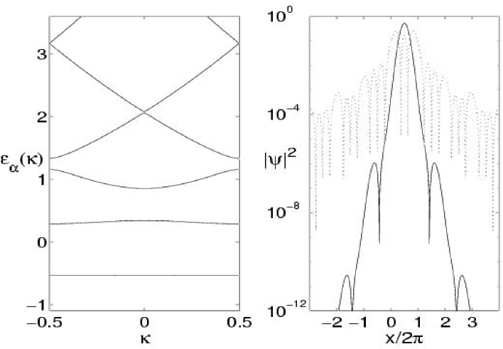
Figure 1.2: Left panel – lowest energy bands $\epsilon_{\alpha}(\kappa)$ for the potential $V(x)=\cos(x)$ with parameters $\hbar=1$ and $m=1$. Right panel – associated Wannier states $\psi_{0,0}$ (solid line) and $\psi_{1,0}$ (dotted line).

The localization property of the Wannier states suggests to use them as a basis for calculating the matrix elements of the Wannier-Stark Hamiltonian (1.1). (Note that the field-free Hamiltonian (1.5) is diagonal in the band index $\alpha$.) The tight-binding Hamiltonian is deduced in the following way. Considering a particular band $\alpha$, one takes into account only the main and the first diagonals of the Hamiltonian $H_{0}$. From the field term $x$ only the diagonal part is taken into account. Then, denoting the Wannier states resulting from the $\alpha$-th band by $|l\rangle$, the tight-binding Hamiltonian reads

$$H_{TB}=\sum_{l}(\bar{\epsilon}_{\alpha}+dFl)\,|l\rangle\langle l|+\frac{\Delta_{\alpha}}{4}\,\big{(}\,|l+1\rangle\langle l|+|l\rangle\langle l+1|\,\big{)}\;.$$ (1.10)

The Hamiltonian (1.10) can be easily diagonalized which yields the spectrum $E_{\alpha,l}=\bar{\epsilon}_{\alpha}+dFl$ with the eigenstates

$$|\Psi_{\alpha,l}\rangle=\sum_{m}J_{m-l}\Big{(}\frac{\Delta_{\alpha}}{2dF}\Big{)}|m\rangle\;.$$ (1.11)

Thus, all states are localized and the spectrum is the discrete Wannier-Stark ladder (1.3).

The obtained result has a transparent physical meaning. When $F=0$ the energy levels of Wannier states $|l\rangle$ coincide and the tunneling couples them into Bloch waves $|\kappa\rangle=\sum_{l}\exp({\rm i}\kappa l)|l\rangle$. Correspondingly, the infinite degeneracy of the level $\bar{\epsilon}_{\alpha}$ is removed, producing the Bloch band  $\epsilon_{\alpha}(\kappa)=\bar{\epsilon}_{\alpha}+(\Delta_{\alpha}/2)\cos(d\kappa).$ When $F\neq 0$ the Wannier levels are misaligned and the tunneling is suppressed. As a consequence, the Wannier-Stark state involves (effectively) a finite number of Wannier states, as indicated by Eq. (1.11). It will be demonstrated later on that for the low-lying bands Eq. (1.3) and Eq. (1.11) approximate quite well the real part of the complex Wannier-Stark spectrum and the resonance Wannier-Stark functions $\Psi_{\alpha,l}(x)$, respectively. The main drawback of the model, however, is its inability to predict the imaginary part of the spectrum (i.e. the lifetime of the Wannier-Stark states), which one has to estimate from an independent calculation. Usually this is done with the help of Landau-Zener theory.

1.3 Landau-Zener tunneling

Let us address the following question: if we take an initial state in the form of a Bloch wave with quasimomentum $\kappa$, what will be the time evolution of this state when the external static field is switched on?

The common approach to this problem is to look for the solution as the superposition of Houston functions [78]

$$\psi(x,t)=\sum_{\alpha}c_{\alpha}(t)\psi_{\alpha}(x,t)\;,$$ (1.12)

$$\psi_{\alpha}(x,t)=\exp\left(-\frac{\rm i}{\hbar}\int_{0}^{\rm t}{\rm d}t^{\prime}\epsilon_{\alpha}(\kappa^{\prime})\right)\phi_{\alpha,\kappa^{\prime}}(x)\;,$$ (1.13)

where $\phi_{\alpha,\kappa^{\prime}}(x)$ is the Bloch function with the quasimomentum $\kappa^{\prime}$ evolving according to the classical equation of motion $\dot{p}=-F$, i.e $\kappa^{\prime}=\kappa-Ft/\hbar$. Substituting Eq. (1.12) into the time-dependent Schrödinger equation with the Hamiltonian (1.1), we obtain

$${\rm i}\hbar\,\dot{c}_{\alpha}=F\sum_{\beta}X_{\alpha,\beta}(\kappa^{\prime})\exp\left(-\frac{\rm i}{\hbar}\int_{0}^{\rm t}{\rm d}t^{\prime}[\epsilon_{\alpha}(\kappa^{\prime})-\epsilon_{\beta}(\kappa^{\prime})]\right)c_{\beta}\;,$$ (1.14)

where $X_{\alpha,\beta}(\kappa)={\rm i}\int{\rm d}x\,\chi^{*}_{\alpha,\kappa}(x)\,\partial/\partial\kappa\,X_{\beta,\kappa}(x)$. Neglecting the interband coupling, i.e. $X_{\alpha,\beta}=0$ for $\alpha\neq\beta$, we have

$$c_{\beta}(t)\approx 0\quad{\rm for}\quad\alpha\neq\beta\qquad{\rm and}\qquad{\rm i}\hbar\,\dot{c}_{\alpha}=F\,X_{\alpha,\alpha}(\kappa^{\prime})\,c_{\alpha}\;.$$ (1.15)

This solution is the essence of the so-called single-band approximation. We note that within this approximation one can use the Houston functions (1.13) to construct the localized Wannier-Stark states similar to those obtained with the help of the tight-binding model.

The correction to the solution (1.15) is obtained by using the formalism of Landau-Zener tunneling. In fact, when the quasimomentum $\kappa^{\prime}$ explores the Brillouin zone, the adiabatic transition occurs at the points of “avoided” crossings between the adjacent Bloch bands [see, for example, the avoided crossing between the 4-th and 5-th bands in Fig. 1.2(a) at $\kappa=0$]. Semiclassically, the probability of this transition is given by

$$P\approx\exp\left(-\frac{\pi\Delta^{2}_{\alpha,\beta}}{8\hbar(|\epsilon^{\prime}_{\alpha}|+|\epsilon^{\prime}_{\beta}|)F}\right)\;,$$ (1.16)

where $\Delta_{\alpha,\beta}$ is the energy gap between the bands and $\epsilon^{\prime}_{\alpha}$, $\epsilon^{\prime}_{\beta}$ stand for the slope of the bands at the point of avoided crossing in the limit $\Delta_{\alpha,\beta}\rightarrow 0$ [79]. In a first approximation, one can assume that the adiabatic transition occurs once for each Bloch cycle $T_{B}=2\pi\hbar/dF$. Then the population of the $\alpha$-th band decreases exponentially with the decay time

$$\tau=\hbar/\Gamma_{\alpha}\;,\quad\Gamma_{\alpha}=a_{\alpha}F\exp(-b_{\alpha}/F)\;,$$ (1.17)

where $a_{\alpha}$ and $b_{\alpha}$ are band-dependent constants.

In conclusion, within the approach described above one obtains from each Bloch band a set of localized states with energies given by Eq. (1.3). However, these states have a finite lifetime given by Eq. (1.17). It will be shown in Sec. 3.1 that the estimate (1.17) is, in fact, a good “first order” approximation for the lifetime of the metastable Wannier-Stark states.

1.4 Experimental realizations

We proceed with experimental realizations of the Wannier-Stark Hamiltonian (1.1). Originally, the problem was formulated for a solid state electron system with an applied external electric field, and in fact, the first measurements concerning the existence of the Wannier-Stark ladder dealt with photo-absorption in crystals [80]. Although this system seems convenient at first glance, it meets several difficulties because of the intrinsic multi-particle character of the system. Namely, the dynamics of an electron in a solid is additionally influenced by electron-phonon and electron-electron interactions. In addition, scattering by impurities has to be taken into account. In fact, for all reasonable values of the field, the Bloch time (1.2) is longer than the relaxation time, and therefore neither Bloch oscillations nor Wannier-Stark ladders have been observed in solids yet.

One possibility to overcome these problems is provided by semiconductor superlattices [81], which consists of alternating layers of different semiconductors, as for example, $GaAs$ and $Al_{x}Ga_{1-x}As$. In the most simple approach, the wave function of a carrier (electron or hole) in the transverse direction of the semiconductor superlattice is approximated by a plane wave for a particle of mass $m^{*}$ (the effective mass of the electron in the conductance or valence bands, respectively). In the direction perpendicular to the semiconductor layers (let it be $x$-axis) the carrier “sees” a periodic sequence of potential barriers

$$V(x)=\left\{\begin{array}[]{ll}V_{0}&\quad{\rm if}\quad\exists\ l\in\mathbb{Z}\quad{\rm with}\quad|x-ld|<a/2\\ \ 0\;,&\quad{\rm else}\end{array}\right.\;,$$ (1.18)

where the height of the barrier $V_{0}$ is of the order of 100 meV and the period $d\sim 100$ Å. Because the period of this potential is two orders of magnitude larger than the lattice period in bulk semiconductor, the Bloch time is reduced by this factor and may be smaller than the relaxation time. Indeed, semiconductor superlattices were the first systems where Wannier-Stark ladders were observed [82, 83, 84] and Bloch oscillations have been measured in four-wave-mixing experiments [85, 86] as proposed in [87]. In the following years, many facets of the topics have been investigated. Different methods for the observation of Bloch oscillation have been applied [88, 89, 90, 91], and nowadays it is possible to detect Bloch oscillations at room temperature [92], to directly measure [93] or even control [94] their amplitude. Wannier-Stark ladders have been found in a variety of superlattice structures [95, 96, 97, 98, 99], with different methods [100, 101]. The coupling between different Wannier-Stark ladders [102, 103, 104, 105, 106], the influence of scattering [107, 108, 109], the relation to the Franz-Keldysh effect [110, 111, 112], the influence of excitonic interactions [113, 114, 115, 116, 117] and the role of Zener tunneling [118, 119, 120, 121] have been investigated. Altogether, there is a large variety of interactions which affect the dynamics of the electrons in semiconductor superlattices, and it is still quite complicated to assign which effect is due to which origin.

A second experimental realization of the Wannier-Stark Hamiltonian is provided by cold atoms in optical lattices. The majority of experiments with optical lattices deals with neutral alkali atoms such as lithium [122], sodium [123, 124, 125], rubidium [126, 127, 128] or cesium [129, 130, 131], but also optical lattices for argon have been realized [132]. The description of the atoms in an optical lattice is rather simple. One approximately treats the atom as a two-state system which is exposed to a strongly detuned standing laser wave. Then the light-induced force on the atom is described by the potential [133, 134]

$$V(x)=\frac{\hbar\Omega_{R}^{2}}{4\delta}\cos^{2}(k_{L}x)\,,$$ (1.19)

where $\hbar\Omega_{R}$ is the Rabi frequency (which is proportional to the product of the dipole matrix elements of the optical transition and the amplitude of the electric component of the laser field), $k_{L}$ is the wave number of the laser, and $\delta$ is the detuning of the laser frequency from the frequency of the atomic transition.

In addition to the optical forces, the gravitational force acts on the atoms. Therefore, a laser aligned in vertical direction yields the Wannier-Stark Hamiltonian

$$H=\frac{p^{2}}{2m}+\frac{\hbar\Omega_{R}^{2}}{8\delta}\,\cos(2k_{L}x)+mgx\;,$$ (1.20)

where $m$ is the mass of the atom and $g$ the gravitational constant. An approach where one can additionally vary the strength of the constant force is realized by introducing a tunable frequency difference between the two counter-propagating waves which form the standing laser wave. If this difference $\delta\omega$ increases linearly in time, $\delta\omega(t)=2k_{L}at$, the two laser waves gain a phase difference which increases quadratically in time according to $\delta\phi(t)=k_{L}at^{2}$. The superposition of both waves then yields an effective potential $V(x,t)=(\hbar\Omega_{R}^{2}/4\delta)\cos^{2}[k_{L}(x-at^{2}/2)]$, which in the rest frame of the potential also yields the Hamiltonian (1.20) with the gravitational force $g$ substituted by $a$. The atom-optical system provides a much cleaner realization of the single particle Wannier-Stark Hamiltonian (1.1) than the solid state systems. No scattering by phonons or lattice impurities occurs. The atoms are neutral and therefore no excitonic effects have to be taken into account. Finally, the interaction between the atoms can be neglected in most cases which justifies a single particle description of the system. Indeed, Wannier-Stark ladders, Bloch oscillations and Zener tunneling have been measured in several experiments in optical lattices [123, 124, 129, 136, 137, 138].

Besides the semiconductor and optical lattices, different attempts have been made to find the Wannier-Stark ladder and Bloch oscillations in other systems like natural superlattices, optical and acoustical waveguides, etc. [139, 140, 141, 142, 143, 144, 145, 146, 147, 148]. However, here we denote them mainly for completeness. In the applications of the theory to real systems we confine ourselves to optical lattices and semiconductor superlattices.

A final remark of this section concerns the choice of the independent parameters of the systems. In fact, by using an appropriate scaling, four main parameters of the physical systems – the particle mass $m$, the period of the lattice $d$, the amplitude of the periodic potential $V_{0}$ and the amplitude of the static force $F$ – can be reduced to two independent parameters. In what follows we use the scaling which sets $m=1$, $V_{0}=1$ and $d=2\pi$. Then the independent parameters of the system are the scaled Planck constant $\hbar^{\prime}$ (entering the momentum operator) and the scaled static force $F^{\prime}$. In particular, for the system (1.20) the scaling $x^{\prime}=2k_{L}x$, $H^{\prime}=H/V_{0}$ ($V_{0}=\hbar^{\prime}\Omega_{R}^{2}/4\delta$) gives

$$\hbar^{\prime}=\left(\frac{8\omega_{\rm rec}\delta}{\Omega^{2}_{R}}\right)^{1/2}\;,\quad\omega_{\rm rec}=\frac{\hbar k^{2}_{L}}{2m}\;,$$ (1.21)

i.e. the scaled Planck constant is inversely proportional to the intensity of the laser field. For the semiconductor superlattice, the scaled Planck constant is $\hbar^{\prime}=2\pi\hbar/d\sqrt{m^{*}V_{0}}$.

1.5 This work

In this work we describe a novel approach to the Wannier-Stark problem which has been developed by the authors during the last few years [149, 150, 151, 152, 153, 154, 155, 156, 157, 158, 159, 160, 161, 162, 163, 164]. By using this approach, one finds the complex spectrum (1.3) as the poles of a rigorously constructed scattering matrix. The suggested method is very efficient from the numerical points of view and has proven to be a powerful tool for an analysis of the Wannier-Stark states in different physical systems.

The review consists of two parts. The first part, which includes chapters 2-3, deals with the case of a dc field. After introducing a scattering matrix for the Wannier-Stark system we describe the basic properties of the Wannier-Stark states, such as lifetime, localization of the wave function, etc., and analyze their dependence on the magnitude of the static field. A comparison of the theoretical predictions with some recent experimental results is also given.

In the second part (chapters 4-7) we study the case of combined ac-dc fields:

$$H=\frac{p^{2}}{2m}+V(x)+Fx+F_{\omega}x\cos(\omega t)\;.$$ (1.22)

We show that the scattering matrix introduced for the case of dc field can be extended to the latter case, provided that the period of the driving field $T_{\omega}=2\pi/\omega$ and the Bloch period (1.1) are commensurate, i.e. $qT_{B}=pT_{\omega}$ with $p,q$ being integers. Moreover, the integer $q$ in the last equation appears as the number of scattering channels. The concept of the metastable quasienergy Wannier-Bloch states is introduced and used to analyze the dynamical and spectral properties of the system (1.22). Although the method of the quasienergy Wannier-Bloch states is formally applicable only to the case of “rational” values of the driving frequency (in the sense of equation $T_{\omega}/T_{B}=q/p$), the obtained results can be well interpolated for arbitrary values of $\omega$.

The last chapter of the second part of the work deals with the same Hamiltonian (1.22) but considers a very different topic. In chapters 2-6 the system parameters are assumed to be in the deep quantum region (which is actually the case realized in most experiments with semiconductors and optical lattices). In chapter 7, we turn to the semiclassical region of the parameters, where the system (1.22) exhibits chaotic scattering. We perform a statistical analysis of the complex (quasienergy) spectrum of the system and compare the results obtained with the prediction of random matrix theory for chaotic scattering.

To conclude, it is worth to add few words about notations. Through the paper we use low case $\phi$ to denote the Bloch states, which are eigenstates of the field free Hamiltonian (1.5). The Wannier-Stark states, which solve the eigenvalue problem with Hamiltonian (1.1) and which are our main object of interest, are denoted by capital $\Psi$. These states should not be mismatched with the Wannier states (1.8) denoted by low case $\psi$. Besides the Bloch, Wannier, and Wannier-Stark states we shall introduce later on the Wannier-Bloch states. These states generalize the notion of Bloch states to the case of nonzero static field and are denoted by capital $\Phi$. Thus we always use capital letters ($\Psi$ or $\Phi$) to refer to the eigenfunctions for $F\neq 0$ and low case letter ($\psi$ or $\phi$) in the case of zero static field, as summarized in the table below.

function	name		dc-field
$\phi_{\alpha,\kappa}(x)$	Bloch	delocalized eigenfunctions of the Hamiltonian $H_{0}$	$F=0$
$\psi_{\alpha,l}(x)$	Wannier	dual localized basis functions	$F=0$
$\Psi_{\alpha,l}(x)$	Wannier-Stark	resonance eigenfunctions of the Hamiltonian $H_{W}$	$F\neq 0$
$\Phi_{\alpha,\kappa}(x)$	Wannier-Bloch	res. eigenfunctions of the evolution operator $U(T_{B})$	$F\neq 0$

Chapter 2 Scattering theory for Wannier-Stark systems

In this work we reverse the traditional view in treating the two contributions of the potential to the Wannier-Stark Hamiltonian

$$H_{W}=\frac{p^{2}}{2}+V(x)+Fx,\quad V(x+2\pi)=V(x)\;.$$ (2.1)

Namely, we will now consider the external field $Fx$ as part of the unperturbed Hamiltonian and the periodic potential as a perturbation, i.e. $H_{W}=H_{0}+V(x)$, where $H_{0}=p^{2}/2+Fx$. The combined potential $V(x)+Fx$ cannot support bound states, because any state can tunnel through a finite number of barriers and finally decay in the negative $x$-direction ($F>0$). Therefore we treat this system using scattering theory. We then have two sets of eigenstates, namely the continuous set of scattering states, whose asymptotics define the S-matrix $S(E)$, and the discrete set of metastable resonance states, whose complex energies $\mathcal{E}=E-{\rm i}\Gamma/2$ are given by the poles of the S-matrix. Due to the periodicity of the potential $V(x)$, the resonances are arranged in Wannier-Stark ladders of resonances. The existence of the Wannier-Stark ladders of resonances in different parameter regimes has been proven, e.g., in [25, 26, 27, 28].

2.1 S-matrix and Floquet-Bloch operator

The scattering matrix $S(E)$ is calculated by comparing the asymptotes of the scattering states $\Psi_{S}(E)$ with the asymptotes of the “unscattered” states $\Psi_{0}(E)$, which are the eigenstates of the “free” Hamiltonian

$$H_{0}=\frac{p^{2}}{2}+Fx\,,\quad F>0.$$ (2.2)

In configuration space, the $\Psi_{0}(E)$ are Airy functions

$$\Psi_{0}(x;E)\sim{\rm Ai}\left(\xi-\xi_{0}\right)\longrightarrow(-\pi^{2}\xi)^{-1/4}\sin\left(\zeta+\pi/4\right)\;.$$ (2.3)

where $\xi=ax$, $\xi_{0}=aE/F$, $a=(2F/\hbar^{2})^{1/3}$, and $\zeta=\frac{2}{3}\,(-\xi)^{3/2}$ [165]. Asymptotically the scattering states $\Psi_{S}(E)$ behave in the same way, however, they have an additional phase shift $\varphi(E)$, i.e. for $x\rightarrow-\infty$ we have

$$\Psi_{S}(x;E)\longrightarrow(-\pi^{2}\xi)^{-1/4}\,{\rm sin}\left[\,\zeta+\pi/4+\varphi(E)\right]\,.$$ (2.4)

Actually, in the Stark case it is more convenient to compare the momentum space instead of the configuration space asymptotes. (Indeed, it can be shown that both approaches are equivalent [160, 164].) In momentum space the eigenstates (2.3) are given by

$$\Psi_{0}(k;E)={\rm exp}\left[{\rm i}\left(\frac{\hbar^{2}k^{3}}{6F}-\frac{Ek}{F}\right)\,\right].$$ (2.5)

For $F>0$ the direction of decay is the negative $x$-axis, so the limit $k\rightarrow-\infty$ of $\Psi_{0}(k;E)$ is the outgoing part and the limit $k\rightarrow\infty$ the incoming part of the free solution.

The scattering states $\Psi_{S}(E)$ solve the Schrödinger equation

$$H_{W}\,\Psi_{S}(E)=E\,\Psi_{S}(E)\,$$ (2.6)

with $H_{W}=H_{0}+V(x)$. (By omitting the second argument of the wave function, we stress that the equation holds both in the momentum and coordinate representations.) Asymptotically the potential $V(x)$ can be neglected and the scattering states are eigenstates of the free Hamiltonian (2.2). In other words, we have

$$\lim_{k\rightarrow\pm\infty}\Psi_{S}(k;E)\,={\rm exp}\left[{\rm i}\left(\frac{\hbar^{2}k^{3}}{6F}-\frac{Ek}{F}\pm\varphi(E)\right)\right]\,.$$ (2.7)

With the help of Eqs. (2.5) and (2.7) we get

$$S(E)=\lim_{k\rightarrow\infty}\frac{\Psi_{S}(-k;E)}{\Psi_{0}(-k;E)}\,\frac{\Psi_{0}(k;E)}{\Psi_{S}(k;E)}\,,$$ (2.8)

which is the definition we use in the following. In terms of the phase shifts $\varphi(E)$ the S-matrix obviously reads $S(E)=\exp[-{\rm i}2\varphi(E)]$ and, thus, it is unitary.

To proceed further, we use a trick inspired by the existence of the space-time translational symmetry of the system, the so-called electric translation [166]. Namely, instead of analyzing the spectral problem (2.6) for the Hamiltonian, we shall analyze the spectral properties of the evolution operator over a Bloch period

$$U=\exp\left(-\frac{{\rm i}}{\hbar}H_{W}T_{B}\right)\;,\quad T_{B}=\frac{\hbar}{F}\;.$$ (2.9)

Using the gauge transformation, which moves the static field into the kinetic energy, the operator (2.9) can be presented in the form

$$U={\rm e}^{-{\rm i}x}\,\widetilde{U}\;,$$ (2.10)

$$\widetilde{U}=\widehat{\rm exp}\left(-\frac{\rm i}{\hbar}\int_{0}^{T_{B}}\left[\frac{(p-Ft)^{2}}{2}+V(x)\right]\,{\rm d}t\right)\;,$$ (2.11)

where the hat over the exponential function denotes time ordering . The advantage of the operator $U$ over the Hamiltonian $H_{W}$ is that it commutes with the translational operator and, thus, the formalism of the quasimomentum can be used. Besides this, the evolution operator also allows us to treat the combined case of an ac-dc field, which will be the topic of the second part of this work.

There is a one to one correspondence between the eigenfunctions of the Hamiltonian and the eigenfunctions of the evolution operator. Indeed, let $\Psi_{S}(x;E)$ be an eigenfunction of $H_{W}$ corresponding to the energy $E$. Then the function

$$\Phi_{S}(x;\lambda,\kappa)=\sum_{l}\exp(+{\rm i}2\pi l\kappa)\Psi_{S}(x-2\pi l;E)$$ (2.12)

is a Bloch-like eigenfunction of $U$ corresponding to the eigenvalue $\lambda=\exp(-{\rm i}ET_{B}/\hbar)$, i.e.

$$U\Phi_{S}(\lambda,\kappa)=\lambda\Phi_{S}(\lambda,\kappa)\;,\quad\lambda=\exp(-{\rm i}E/F)\;.$$ (2.13)

Equation (2.13) simply follows from the continuous time evolution of the function (2.12), which is $\Phi_{S}(x;\lambda,\kappa,t)=\sum_{l}\exp(+{\rm i}2\pi l\kappa)\exp[-{\rm i}(E+2\pi Fl)t/\hbar]\Psi_{S}(x-2\pi l;E)$, or

$$\Phi_{S}(\lambda,\kappa,t)=\exp(-{\rm i}Et/\hbar)\Phi_{S}(\lambda,\kappa-Ft/\hbar)\;.$$ (2.14)

Let us also note that the quasimomentum $\kappa$ does not enter into the eigenvalue $\lambda$. Thus the spectrum of the evolution operator $U$ is degenerate along the Brillouin zone. Besides this, the relation between energy $E$ and $\lambda$ is unique only if we restrict the energy interval considered to the first “energy Brillouin zone”, i.e. $0\leq E\leq 2\pi F$.

When the energy is restricted by this first Brillouin zone, the transformation inverse to (2.12) reads

$$\Psi_{S}(E)=\int_{-1/2}^{1/2}{\rm d}\kappa\,\Phi_{S}(\lambda,\kappa)\;.$$ (2.15)

This relation allows us to use the asymptotes of the Floquet-Bloch solution $\Phi_{S}(\lambda,\kappa)$ instead of the asymptotes of the $\Psi_{S}(E)$ in the S-matrix definition (2.8). In fact, since the functions $\Phi_{S}(x;\lambda,\kappa)$ are Bloch-like solution, they can be expanded in the basis of plane waves:

$$\Phi_{S}(x;\lambda,\kappa)=\sum_{n}C_{S}(n;\lambda,\kappa)\langle x|n+\kappa\rangle\;,\quad\langle x|n+\kappa\rangle=(2\pi)^{-1/2}e^{{\rm i}(n+\kappa)x}\;.$$ (2.16)

From the integral (2.15) the relation $\langle n+\kappa|\Phi_{S}(\lambda,\kappa)\rangle=\langle n+\kappa|\Psi_{S}(E)\rangle$ follows directly, i.e. in the momentum representation the functions $\Psi_{S}(k;E)$ and $\Phi_{S}(k;\lambda,\kappa)$ coincide at the points $k=n+\kappa$. Thus we can substitute the asymptotes of $\Phi_{S}(k;\lambda,\kappa)$ in Eq. (2.8). This gives

$$S(E)=\lim_{n\rightarrow\infty}\frac{C_{S}(-n)}{C_{0}(-n)}\,\frac{C_{0}(n)}{C_{S}(n)}\>,$$ (2.17)

where the energy on the right-hand side of the equation enters implicitly through the eigenvalue $\lambda=\exp(-{\rm i}E/F)$. Let us also note that by construction $S(E)$ in Eq. (2.17) does not depend on the particular choice of the quasimomentum $\kappa$. In numerical calculations this provides a test for controlling the accuracy.

2.2 S-matrix: basic equations

Using the expansion (2.16), the eigenvalue equation (2.13) can be presented in matrix form

$$\sum_{n}\widetilde{U}^{(\kappa)}_{m+1,n}C_{S}(n)=\lambda C_{S}(m)\;,$$ (2.18)

where

$$\widetilde{U}^{(\kappa)}_{m,n}=\langle m+\kappa|\,\widetilde{U}\,|n+\kappa\rangle$$ (2.19)

and the unitary operator $\widetilde{U}$ is given in Eq. (2.11). [Deriving Eq. (2.18) from Eq. (2.13), we took into account that in the plane wave basis the momentum shift operator $\exp(-{\rm i}x)$ has the matrix elements $\langle m|\exp(-{\rm i}x)|n\rangle=\delta_{m+1,n}$.] Because $\lambda$ does not depend on the quasimomentum $\kappa$, we can set $\kappa=0$ and shall drop this upper matrix index in what follows.

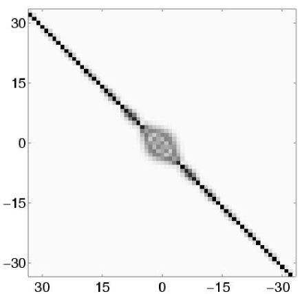
Figure 2.1: Matrix of the Floquet-Bloch operator $U$ for $H_{W}=p^{2}/2+\cos(x)+Fx$ with system parameters $\hbar=0.5$ and $F=0.2$: The absolute values of the elements are shown in a grey scale plot. With increasing indices the matrix tends to a diagonal one.

For $n\rightarrow\pm\infty$, the kinetic term of the Hamiltonian dominates the potential and the matrix $\widetilde{U}$ tends to a diagonal one. This property is exemplified in Fig. 2.1, where we depict the Floquet-Bloch matrix for the potential $V(x)=\cos(x)$. Suppose the effect of the off-diagonals elements can be neglected for $|n|>N$. Then we have

$$\widetilde{U}_{m,n}\approx u_{m}\delta_{m,n}\qquad{\rm for}\,\,|m|,|n|>N\,$$ (2.20)

with

$$u_{m}=\exp\left(-\frac{\rm i}{2\hbar}\int_{0}^{T_{B}}{(\hbar m-Ft)}^{2}\,{\rm d}t\right)=\exp\left(\frac{\rm i\hbar^{2}}{6F}\left[(m-1)^{3}-m^{3}\right]\right)\;.$$ (2.21)

For the unscattered states $\Phi_{0}(\lambda)$ the formulas (2.20) hold exactly for any $m$ and, given a energy $E$ or $\lambda=\exp(-iE/F)$, the eigenvalue equation can be solved to yield the discrete version of the Airy function in the momentum representation: $C_{0}(m)=\exp({\rm i}\hbar^{2}m^{3}/6F-{\rm i}Em/F)$. With the help of the last equation we have

$$\frac{C_{0}(n)}{C_{0}(-n)}=\exp\left[{\rm i}\,\frac{\hbar^{2}n^{3}}{3F}-{\rm i}\frac{2En}{F}\right]\;,$$ (2.22)

which can be now substituted into the S-matrix definition (2.17).

We proceed with the scattering states $\Phi_{S}(\lambda)$. Suppose we order the $C_{S}$ with indices increasing from bottom to top. Then we can decompose the vector $C_{S}$ into three parts,

$$C_{S}=\left(\begin{array}[]{l}C_{S}^{(+)}\\[2.84526pt] C_{S}^{(0)}\\[2.84526pt] C_{S}^{(-)}\end{array}\right)\;,$$ (2.23)

where $C_{S}^{(+)}$ contains the coefficients for $n>N$, $C_{S}^{(-)}$ contains the coefficients for $n<-N\!-\!1$ and $C_{S}^{(0)}$ contains all other coefficients for $-N\!-\!1\leq n\leq N$. The coefficients of $C_{S}^{(+)}$ recursively depend on the coefficient $C_{S}(N)$, via

$$C_{S}(m+1)=(\lambda/u_{m+1})\,C_{S}(m)\qquad{\rm for}\quad m\geq N\,.$$ (2.24)

Analogously, the coefficients of $C_{S}^{(-)}$ recursively depend on $C_{S}(-N-1)$, via

$$C_{S}(m)=(u_{m+1}/\lambda)\,C_{S}(m+1)\qquad{\rm for}\quad m<-N-1\,.$$ (2.25)

Let us define the matrix $W$ as the matrix $\widetilde{U}$, truncated to the size $(2N+1)\times(2N+1)$. Furthermore, let $B_{N}$ be the matrix $W$ accomplished by zero column and row vectors:

$$B_{N}=\left(\begin{array}[]{cc}\vec{0}^{\rm t}&0\\ W&\vec{0}\\ \end{array}\right)\;.$$ (2.26)

Then the resulting equation for $C_{S}^{(0)}$ can be written as

$$\left(B_{N}-\lambda\leavevmode\hbox{\small 1\kern-3.8pt\normalsize 1}\right)C_{S}^{(0)}=-u_{N+1}\,C_{S}(N+1)\,e^{1}\,,$$ (2.27)

where $e^{1}$ is a vector of the same length as $C_{S}^{(0)}$, with the first element equal to one and all others equal to zero. For a given $\lambda$, Eq. (2.27) matches the asymptotes $C_{S}^{(+)}$ and $C_{S}^{(-)}$ by linking $C_{S}^{(+)}$, via $C_{S}(N+1)$ and Eq. (2.24), to $C_{S}^{(0)}$ and, via $C_{S}(-N-1)$ and Eq. (2.25), to $C_{S}^{(-)}$. Let us now introduce the row vector $e_{1}$ with all elements equal to zero except the last one, which equals one. Multiplying $e_{1}$ with $C_{S}^{(0)}$ yields the last element of the latter one, i.e. $C_{S}(-N-1)$. Assuming that $\lambda$ is not an eigenvalue of the matrix $B_{N}$ (this case is treated in the next section) we can multiply Eq. (2.27) with the inverse of $(B_{N}-\lambda\leavevmode\hbox{\small 1\kern-3.8pt\normalsize 1})$, which yields

$$\frac{C_{S}(-N-1)}{C_{S}(N+1)}=-u_{N+1}\,e_{1}\left[\,B_{N}-{\rm e}^{-{\rm i}E/F}\,\leavevmode\hbox{\small 1\kern-3.8pt\normalsize 1}\,\right]^{-1}e^{1}\;.$$ (2.28)

Finally, substituting Eq. (2.22) and Eq. (2.28) into Eq. (2.17), we obtain

$$S(E)=\lim_{N\rightarrow\infty}A(N+1)\,e_{1}\left[\,B_{N}-{\rm e}^{-{\rm i}E/F}\,\leavevmode\hbox{\small 1\kern-3.8pt\normalsize 1}\,\right]^{-1}e^{1}\;,$$ (2.29)

with a phase factor $A(N)=-u_{N}C_{0}(N)/C_{0}(-N)$, which ensures the convergence of the limit $N\rightarrow\infty$. The derived Eq. (2.29) defines the scattering matrix of the Wannier-Stark system and is one of our basic equations.

To conclude this section, we note that Eq. (2.29) also provides a direct method to calculate the so-called Wigner delay time

$$\tau(E)=-{\rm i}\,\hbar\,\frac{\partial\ln S(E)}{\partial E}=-2\hbar\,\frac{\partial\varphi(E)}{\partial E}\;.$$ (2.30)

As shown in Ref. [153],

$$\tau(E)=\lim_{N\rightarrow\infty}\frac{\hbar}{F}\left[\,\left(C_{S}^{(0)},C_{S}^{(0)}\right)-2(N+1)\,\right]\;.$$ (2.31)

Thus, one can calculate the delay time from the norm of the $C_{S}^{(0)}$, which is preferable to (2.30) from the numerical point of view, because it eliminates an estimation of the derivative. In the subsequent sections, we shall use the Wigner delay time to analyze the complex spectrum of the Wannier-Stark system.

2.3 Calculating the poles of the S-matrix

Let us recall the S-matrix definitions for the Stark system,

$$S(E) = \lim_{k\rightarrow\infty}\frac{\Psi_{S}(-k;E)}{\Psi_{S}(k;E)}\,\frac{\Psi_{0}(k;E)}{\Psi_{0}(-k;E)}=\lim_{n\rightarrow\infty}\frac{C_{S}(-n)}{C_{S}(n)}\,\frac{C_{0}(n)}{C_{0}(-n)}\;.$$ (2.32)

The S-Matrix is an analytic function of the (complex) energy, and we call its isolated poles located in the lower half of the complex plane, i.e. those which have an imaginary part less than zero, resonances. In terms of the asymptotes of the scattering states, resonances correspond to scattering states with purely outgoing asymptotes, i.e. with no incoming wave. (These are the so-called Siegert boundary conditions [168].) As one can see directly from (2.22), poles cannot arise from the contributions of the free solutions. In fact, $C_{0}(n)/C_{0}(-n)$ decreases exponentially as a function of $n$ for complex energies $\mathcal{E}=E-{\rm i}\Gamma/2$. Therefore, poles can arise only from the scattering states $C_{S}$.

Actually, we already noted the condition for poles in the previous section. In the step from equation (2.27) to the S-matrix formula (2.29) we needed to invert the matrix $(B_{N}-\lambda\leavevmode\hbox{\small 1\kern-3.8pt\normalsize 1})$. We therefore excluded the case when $\lambda$ is an eigenvalue of $B_{N}$. Let us treat it now. If $\lambda$ is an eigenvalue of $B_{N}$, the equation defining $C^{(0)}_{S}$ then reads

$$\left(B_{N}-\lambda\leavevmode\hbox{\small 1\kern-3.8pt\normalsize 1}\right)C_{S}^{(0)}=0\;.$$ (2.33)

The scattering state $C_{S}$ we get contains no incoming wave, i.e. it fulfills the Siegert boundary condition. In fact, the first element $C^{(0)}_{S}(N)$ is equal to zero, which follows directly from the structure of $B_{N}$, and consequently $C_{S}^{(+)}=0$. In addition, the eigenvalues fulfill $|\lambda|\leq 1$, which in terms of the energy $\mathcal{E}=E-{\rm i}\Gamma/2$ means $\Gamma\geq 0$. Let us also note that, according to Eq. (2.25), the outgoing wave $C_{S}^{(-)}$ diverges exponentially as $C_{S}^{(-)}(n)\sim|\lambda|^{-n}$.

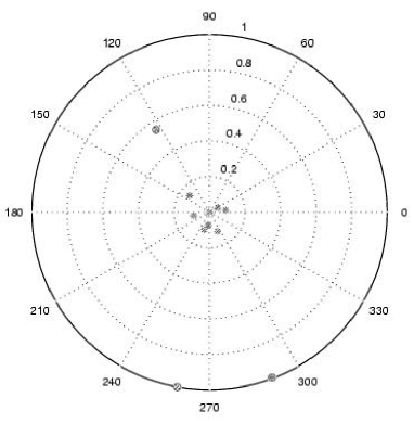
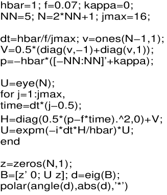
Figure 2.2: The eigenvalues $\lambda$ of the matrix $B_{N}$ calculated for system (2.1) with $V(x)=\cos x$, $\hbar=1$ and $F=0.07$. The numerical parameters are $N=5$, $j_{\rm max}=16$ and $\kappa=0$. The eigenvalues corresponding to the first three Wannier-Stark ladders are marked by circles. On the right to the figure is the matlab source code which generates the depicted data.

Equation (2.33) provides the basis for a numerical calculation of the Wannier-Stark resonances. A few words should be said about the numerical algorithm. The time evolution matrix (2.11) can be calculated by using $2N+1$ plane wave basis states $\langle x|n\rangle=(2\pi)^{-1/2}\exp({\rm i}nx)$ via

$$\widetilde{U}^{(\kappa)}\approx\prod_{j=1}^{j_{\rm max}}\exp\left(-\frac{{\rm i}}{\hbar}\widetilde{H}^{(\kappa)}(t_{j})\Delta t\right)$$ (2.34)

where $t_{j}=(j\!-\!1/2)\Delta t$, $\Delta t=T_{B}/j_{\rm max}$ and $\widetilde{H}^{(\kappa)}(t_{j})$ is the truncated matrix of the operator $\widetilde{H}^{(\kappa)}(t)=(p-Ft+\hbar\kappa)^{2}/2+V(x)$. Then, by adding zero elements, we obtain the matrix $B_{N}$ and calculate its eigenvalues $\lambda$. The resonance energies are given by $\mathcal{E}={\rm i}F\ln\lambda$. As an example, Fig 2.2 shows the eigenvalues $\lambda_{\alpha}$ in the polar representation for the system (2.1) with $V(x)=\cos x$. Because of the numerical error (introduced by truncation procedure and round error) not all eigenvalues correspond to the S-matrix poles. The “true” $\lambda$ can be distinguished from the “false” $\lambda$ by varying the numerical parameters $N$, $j_{\rm max}$ and the quasimomentum $\kappa$ (we recall that in the case of dc field $\lambda$ is independent of $\kappa$). The true $\lambda$ are stable against variation of the parameters, but the false $\lambda$ are not. In Fig 2.2, the stable $\lambda$ are marked by circles and can be shown (see next section) to correspond to Wannier-Stark ladders originating from the first three Bloch bands. By increasing the accuracy, more true $\lambda$ (corresponding to higher bands) can be detected.

2.4 Resonance eigenfunctions

According to the results of preceding section, the resonance Bloch-like functions $\Phi_{\alpha,\kappa}$, referred to in what follows as the Wannier-Bloch functions, are given (in the momentum representation) by

$$\Phi_{\alpha,\kappa}(k)=\sum_{n}C_{\alpha}(n)\,\delta(n+\kappa-k)\;.$$ (2.35)

where $C_{\alpha}(n)$ are the elements of the eigenvector of Eq. (2.33) in the limit $N\rightarrow\infty$. The change of the notation $\Phi_{S}(\lambda,\kappa)\rightarrow\Phi_{\alpha,\kappa}$ indicates that from now on we deal with the resonance eigenfunctions corresponding to the discrete (complex) spectrum $\mathcal{E}_{\alpha}$. The Wannier-Stark states $\Psi_{\alpha,l}$, which are the resonance eigenfunction of the Wannier-Stark Hamiltonian $H_{W}$, are calculated by using Eq. (2.14) and Eq. (2.15). In fact, according to Eq. (2.14), the quasimomentum $\kappa$ of the Wannier-Bloch function changes linearly with time and explores the whole Brillouin zone during one Bloch period. Thus, one can obtain the Wannier-Stark states $\Psi_{\alpha,l}$ by calculating the eigenfunction $\Phi_{\alpha,\kappa}$ of the evolution operator $U$ for, say, $\kappa=0$ and propagating it over the Bloch period. (Additionally, the factor $\exp(-{\rm i}\mathcal{E}_{\alpha}t/\hbar)$ should be compensated.) We used the discrete version of the continuous evolution operator, given by (2.34) with the upper limit $j_{\rm max}$ substituted by the actual number of timesteps. Resonance Wannier-Stark functions corresponding to two most stable resonances are shown in Fig. 2.3.

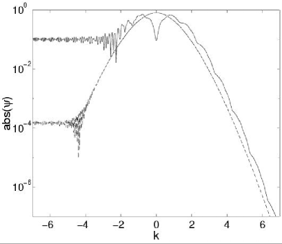
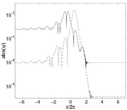
Figure 2.3: Resonance wave functions of the two most stable resonances of system (2.1) with parameters $\hbar=1$ and $F=0.07$ in momentum and in configuration space. The ground state is plotted as a dashed, the first excited state as a solid line. In the second figure the first excited state is shifted by one space period to enhance the visibility.

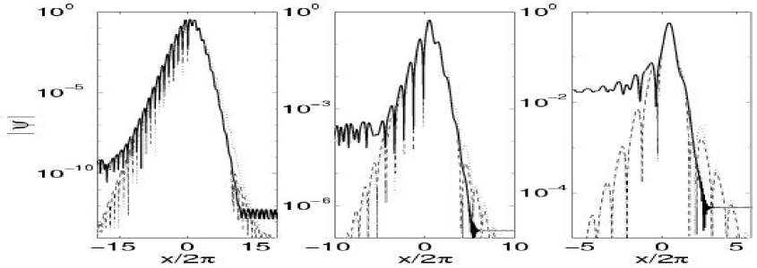
Figure 2.4: Comparison of the wave functions calculated within the different approaches for $\hbar=2$ and $F=0.01,0.03,0.1$, shown on a linear (top) and on a logarithmic scale (bottom). The dotted line is the tight-binding, the dashed line the single-band and the solid line is the scattering result.

The left panel in Fig. 2.3 shows the wave functions in the momentum representation, where the considered interval of $k=p/\hbar$ is defined by the dimension of the matrix $B_{N}$, i.e. $|k|\leq N$. The (faster than exponential) decrease in the positive direction is clearly visible. The tail in the negative direction reflects the decay of resonances. Although it looks to be constant in the figure, its magnitude actually increases exponentially (linearly in the logarithmic scale of the figure) as $k\rightarrow-\infty$. The wave functions in the coordinate representation (right panel) are obtained by a Fourier transform. Similar to the momentum space the resonance wave functions decrease in positive $x$-direction and have a tail in the negative one. Obviously, a finite momentum basis implies a restriction to a domain in space, who’s size can be estimated from energy conservation as $|x|\leq\hbar^{2}N^{2}/2F$. Additionally the Fourier transformation introduces numerical errors due to which the wave functions decay only to some finite value in positive direction. We note, however, that for most practical purposes it is enough to know the Wannier-Stark states in the momentum representation.

Now we discuss the normalization of the Wannier-Stark states. Indeed, because of the presence of the exponentially diverging tail, the wave functions $\Psi_{\alpha,l}(k)$ or $\Psi_{\alpha,l}(x)$ can not be normalized in the usual sense. This problem is easily resolved by noting that for the non-hermitian eigenfunctions (i.e. in the case considered here) the notion of scalar product is modified as

$$\int{\rm d}x\Psi^{*}_{\alpha,l}(x)\Psi_{\alpha,l}(x)\rightarrow\int{\rm d}x\Psi^{L}_{\alpha,l}(x)\Psi^{R}_{\alpha,l}(x)\;,$$ (2.36)

where $\Psi^{L}_{\alpha,l}(x)$ and $\Psi^{R}_{\alpha,l}(x)$ are the left and right eigenfunctions, respectively. In Fig. 2.3 the right eigenfunctions are depicted. The left eigenfunctions can be calculated in the way described above, with the exception that one begins with the left eigenvalue equation $C_{S}^{(0)}\left(B_{N}-\lambda\leavevmode\hbox{\small 1\kern-3.8pt\normalsize 1}\right)=0$ for the row vector $C_{S}^{(0)}$. In the momentum representation, the left function $\Psi^{L}_{\alpha,l}(k)$ coincides with the right one, mirrored relative to $k=0$. (Note that in coordinate space, the absolute values of both states are identical.) In other words, it corresponds to a scattering state with zero amplitude of the outgoing wave. Since for the right wave function a decay in the positive $k$-direction is faster than the increase of the left eigenfunction (being inverted, the same is valid in the negative $k$-direction), the scalar product of the left and right eigenfunctions is finite. In our numerical calculation we typically calculate both functions in the momentum representation and then normalize them according to

$$\int{\rm d}k\Psi^{L}_{\alpha,l}(k)\Psi^{R}_{\beta,n}(k)=\langle\Psi_{\alpha,l}|\Psi_{\beta,n}\rangle=\delta_{\alpha,\beta}^{l,n}\;.$$ (2.37)

(Here and below we use the Dirac notation for the left and right wave functions.) Let us also recall the relations

$$\Psi_{\alpha,l}(x)=\Psi_{\alpha,0}(x-2\pi l)$$ (2.38)

for the wave functions in the coordinate representation and

$$\Psi_{\alpha,l}(k)=\exp({\rm i}2\pi lk)\Psi_{\alpha,0}(k)$$ (2.39)

in the momentum space. Thus it is enough to normalize the function for $l=0$. Then the normalization of the other functions for $l\neq 0$ will hold automatically. For the purpose of future reference we also display a general (not restricted to the first energy Brillouin zone) relation between the Wannier-Bloch and Wannier-Stark states

$$\Psi_{\alpha,l}=\int_{-1/2}^{1/2}{\rm d}\kappa\exp(-{\rm i}2\pi l\kappa)\Phi_{\alpha,\kappa}$$ (2.40)

(compare with Eq. (1.8).

It is interesting to compare the resonance Wannier-Stark states with those predicted by the tight-binding and single-band models. Such a comparison is given in Fig. 2.4, where the ground Wannier-Stark state for the potential $V(x)=\cos x$ is depicted for three different values of the static force $F$. As expected, for small $F$, where the resonance is long-lived, both approximations yield a good correspondence with the exact calculation. (In the limit of very small $F$ the single-band model typically gives a better approximation than the tight-binding model.) In the unstable case, where the resonance state has a visible tail due to the decay, the results differ in the negative direction. On logarithmic scale one can see that the order of magnitude up to which the results coincide is given by the decay tail of the resonances. In the positive $x$-direction the resonance wave functions tend to be stronger localized. It should be noted that in Fig. 2.4 we considered the ground Wannier-Stark states only for moderate values of the static force $F<0.1$. For larger $F$, because of the exponential divergence, the comparison of the resonance Wannier-Stark states with the localized states of the single-band model loses its sense. The same is also true for higher ($\alpha>0$) states. Moreover, the value of $F$, below which the comparison is possible, rapidly decreases with increase of band index $\alpha$.

Chapter 3 Interaction of Wannier-Stark ladders

In this chapter we give a complete description of the dependence of the width $\Gamma$ of the Wannier-Stark resonances on the parameters of the Wannier-Stark Hamiltonian. In scaled units, the Hamiltonian has two independent parameters, the scaled Planck constant $\hbar$ and the field strength $F$. In our analysis we fix the value of $\hbar$ and investigate the width as a function of the field strength. The calculated lifetimes $\tau=\hbar/\Gamma$ are compared with the experimentally measured lifetimes of the Wannier-Stark states.

3.1 Resonant tunneling

To get a first glimpse on the subject, we calculate the resonances for the Hamiltonian (2.1) with $V(x)=\cos x$ for $\hbar=1$. For the chosen periodic potential the field-free Hamiltonian has two bands with energies well below the potential barrier. For the third band, the energy $\epsilon_{2}(\kappa)$ can be larger than the potential height. Therefore, with the field switched on, one expects two long-lived resonance states in each potential well, which are related to the first two bands.

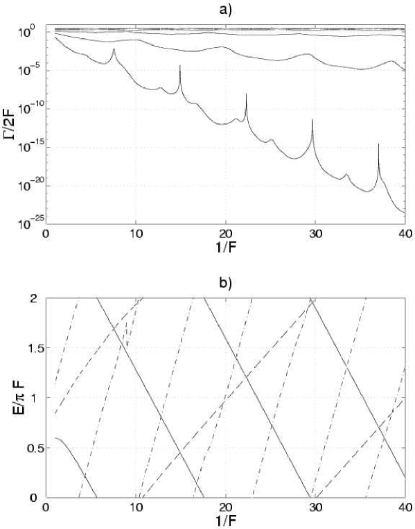
Figure 3.1: a) Resonance width of the $6$ most stable resonances as a function of the inverse field strength $1/F$. b) Energies of the $3$ most stable resonances as a function of $1/F$ (solid line: most stable resonance, dashed line: first excited resonance, dashed dotted line: second excited resonance). Parameters are $V(x)=\cos x$ and $\hbar=1$.

Figure 3.1(a) shows the calculated widths of the six most stable resonances as a function of the inverse field strength $1/F$. The two most stable resonances are clearly separated from the other ones. The second excited resonance can still be distinguished from the others, the lifetime of which is similar. Looking at the lifetime of the most stable state, the most striking phenomenon is the existence of very sharp resonance-like structures, where within a small range of $F$ the lifetime can decrease up to six orders of magnitude. In Fig. 3.1(b), we additionally depict the energies of the three most stable resonances as a function of the inverse field strength. As the Wannier-Stark resonances are arranged in a ladder with spacing $\Delta E=2\pi F$, we show only the first energy Brillouin zone $0<E/F<2\pi$. Let us note that the mean slope of the lines in Fig. 3.1(b) defines the absolute position $E^{*}_{\alpha}$ of the Wannier-Stark resonances in the limit $F\rightarrow 0$. As follows from the single band model, these absolute positions can be approximated by the mean energies $\bar{\epsilon}_{\alpha}$ of the Bloch bands. Depending on the value of $E^{*}_{\alpha}$, we can identify a particular Wannier-Stark resonance either as under- or above-barrier resonance.

Comparing Fig. 3.1(b) with Fig. 3.1(a), we observe that the decrease in lifetime coincides with crossings of the energies of the Wannier-Stark resonances. All three possible crossings manifest themselves in the lifetime: Crossings of the two most stable resonances coincide with the sharpest peaks in the ground state width. The smaller peaks can be found at crossings of the ground state and the second excited state. Finally, crossings of the first and the second excited state fit to the peaks in the width of the first excited state.

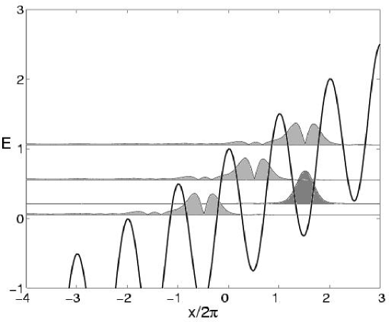
Figure 3.2: Wannier-Stark resonances in different minima of the potential $V(x)=\cos(x)+Fx$: The most stable resonance and some members of the first excited Wannier-Stark ladder are shown. The parameters are $\hbar=1.0$ and $F=0.08$.

The explanation of this effect is the following: Suppose we have a set of resonances which localize in one of the $2\pi$-periodic minima of the potential $V(x)=\cos x+Fx$. Let $\Delta E_{\alpha,\beta}=E_{\alpha}-E_{\beta}$ be the energy difference between two of these states. Now, due to the periodicity of the cosine, each resonance is a member of a Wannier-Stark ladder of resonances, i.e. of a set of resonances with the same width, but with energies separated by $\Delta E=2\pi F$. Figure 3.2 shows an example: The two most stable resonances for one potential minimum are depicted, furthermore two other members of the Wannier-Stark ladder of the first excited resonance. To decay, the ground state has to tunnel three barriers. Clearly, if there is a resonance with nearly the same energy in one of the adjacent minima, this will enhance the decay due to phenomenon of resonant tunneling. The strongest effect will be given for degenerate energies, i.e. for $2\pi Fl=\Delta E_{\alpha,\beta}$, which can be achieved by properly adjusting $F$, because the splitting $\Delta E_{\alpha,\beta}\approx E^{*}_{\beta}-E^{*}_{\alpha}$ is nearly independent of the field strength. For the case shown in Fig. 3.2, such a degeneracy will occur, e.g., for a slightly smaller value $F\approx 1/14.9$ (see Fig. 3.1). Then we have two resonances with the same energies, which are separated by two potential barriers. In the next section we formalize this intuitive picture by introducing a simple two-ladder model.

3.2 Two interacting Wannier-Stark ladders

It is well known that the interaction between two resonances can be well modeled by a two-state system [34, 169, 170, 171]. In this approach the problem reduces to the diagonalization of a $2\times 2$ matrix, where the diagonal matrix elements correspond to the non-interacting resonances. In our case, however, we have ladders of resonances. This fact can be properly taken into account by introducing the diagonal matrix in the form [155, 160]

$$U_{0}=\exp\left(-{\rm i}\,\frac{H_{0}}{F}\right)\;,\quad H_{0}=\left(\begin{array}[]{cc}E_{0}-{\rm i}\Gamma_{0}/2&0\\ 0&E_{1}-{\rm i}\Gamma_{1}/2\end{array}\right)\;.$$ (3.1)

It is easy to see that the eigenvalues $\lambda_{0,1}(F)=\exp[-{\rm i}(E_{0,1}-{\rm i}\Gamma_{0,1}/2]/F)$ of $U_{0}$ correspond to the relative energies of the Wannier-Stark levels and, thus, the matrix $U_{0}$ models two crossing ladders of resonances. Multiplying the matrix $U_{0}$ by the matrix

$$U_{\rm int}=\exp\left[{\rm i}\epsilon\left(\begin{array}[]{cc}0&1\\ 1&0\end{array}\right)\right]=\left(\begin{array}[]{cc}\cos\epsilon&{\rm i}\sin\epsilon\\ {\rm i}\sin\epsilon&\cos\epsilon\end{array}\right)\;,$$ (3.2)

we introduce an interaction between the ladders. The matrix $U_{0}U_{\rm int}$ can be diagonalized analytically, which yields

$$\lambda_{\pm}=\frac{\lambda_{0}+\lambda_{1}}{2}\,\cos\epsilon\pm\left[\left(\frac{\lambda_{0}+\lambda_{1}}{2}\right)^{2}\cos^{2}\epsilon-\lambda_{0}\lambda_{1}\right]^{1/2}\;,\quad\lambda_{\pm}=\exp\left(-{\rm i}\,\frac{E_{\pm}-{\rm i}\Gamma_{\pm}/2}{F}\right)\;.$$ (3.3)

Based on Eq. (3.3) we distinguish the cases of weak, moderate or strong ladder interaction.

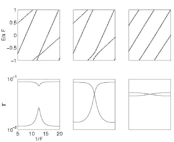
Figure 3.3: Illustration to the two-ladder model. Parameters are $\mathcal{E}_{0}=0.3-{\rm i}1.1\cdot 10^{-2}$, $\mathcal{E}_{1}=0.8-{\rm i}0.9\cdot 10^{-1}$, and $\epsilon=0.2$ (left column), $\epsilon=0.4$ (center), and $\epsilon=\pi/2-0.1$ (right column). Upper panels show the energies $E_{\pm}$, lower panels the widths $\Gamma_{\pm}$.

The value $\epsilon=0$ obviously corresponds to non-interacting ladders. By choosing $\epsilon\neq 0$ but $\epsilon\ll\pi/2$ we model the case of weakly interacting ladders. In this case the ladders show true crossing of the real parts and “anticrossing” of the imaginary parts. Thus the interaction affects only the stability of the ladders. Indeed, for $\epsilon\ll\pi/2$ Eq. (3.3) takes the form

$$\lambda_{\pm}=\lambda_{0,1}\left(1\pm\frac{\epsilon^{2}}{2}\frac{\lambda_{0}+\lambda_{1}}{\lambda_{1}-\lambda_{0}}\right)\;.$$ (3.4)

It follows from the last equation that at the points of crossing (where the phases of $\lambda_{0}$ and $\lambda_{1}$ coincide) the more stable ladder (let it be the ladder with index 0, i.e. $\Gamma_{0}<\Gamma_{1}$ or $|\lambda_{0}|>|\lambda_{1}|$) is destabilized ($|\lambda_{+}|<|\lambda_{0}|$) and, vice versa, the less stable ladder becomes more stable ($|\lambda_{-}|>|\lambda_{1}|$). The case of weakly interacting ladders is illustrated by the left column in Fig. 3.3.

By increasing $\epsilon$ above $\epsilon_{\rm cr}$,

$$\sin^{2}\epsilon_{\rm cr}=\left(\frac{|\lambda_{0}|-|\lambda_{1}|}{|\lambda_{0}|+|\lambda_{1}|}\right)^{2}\;,$$ (3.5)

the case of moderate interaction, where the true crossing of the real parts $E_{\pm}$ is substituted by an anticrossing, is met. As a consequence, the interacting Wannier-Stark ladders exchange their stability index at the point of the avoided crossing (see center column in Fig. 3.3). The maximally possible interaction is achieved by choosing $\epsilon=\pi/2$. Then the eigenvalues of the matrix $U_{0}U_{\rm int}$ are $\lambda_{\pm}=\pm{\rm i}(\lambda_{0}\lambda_{1})^{1/2}$ which corresponds to the “locked” ladders

$$E_{\pm}=(E_{0}+E_{1})/2\pm\pi F/2\;,\quad\Gamma_{\pm}=(\Gamma_{0}+\Gamma_{1})/2\;.$$ (3.6)

In other words, the energy levels of one Wannier-Stark ladder are located exactly in the middle between the levels of the other ladder (right column in Fig. 3.3).

3.3 Wannier-Stark ladders in optical lattices

In the following two sections we give a comparative analysis of the ladder interaction in optical and semiconductor superlattices. It will be shown that the character of the interaction can be qualitatively deduced from the Bloch spectrum of the system.

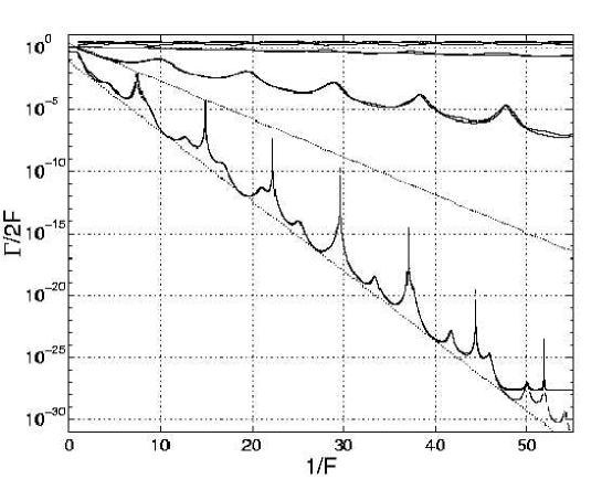
Figure 3.4: Widths of the 6 most stable resonances as a function of the inverse field $F$ for $\hbar=1.0$ (solid lines) compared with the fit data (dashed lines).

We begin with the optical lattice, which realizes the case of a cosine potential (see Sec. 1.4). A characteristic feature of the cosine potential is an exponential decrease of the band gaps as $E\rightarrow\infty$ [see Fig. 1.2(a), for example]. In order to get a satisfactory description of the ladder interaction for $F\neq 0$, it is sufficient to consider only the under-barrier resonances and one or two above-barrier resonances. In particular, for the parameters of Fig. 3.1 it is enough to “keep track” of the resonances belonging to the first three Wannier-Stark ladders. It is also seen in Fig. 3.1 that the case of true crossings of the resonances is realized almost exclusively, i.e. the ladders are weakly interacting (which is another characteristic property of the cosine potential). The behavior of the resonance widths $\Gamma_{\alpha}(F)$ at the vicinity of a particular crossing is captured by Eq. (3.4). Moreover, extending the two-ladder model of the previous section to the three ladder case and assuming the coupling constants in the form

$$\epsilon_{\alpha}=a_{\alpha}\exp(-b_{\alpha}/F)\;,$$ (3.7)

(which is suggested by the semiclassical arguments of Sec. 1.3) the overall behavior of the resonance width can be perfectly reproduced (see Fig. 3.4). The procedure of adjustment of the model parameters $a_{\alpha}$ and $b_{\alpha}$ is carefully described in Ref. [160].

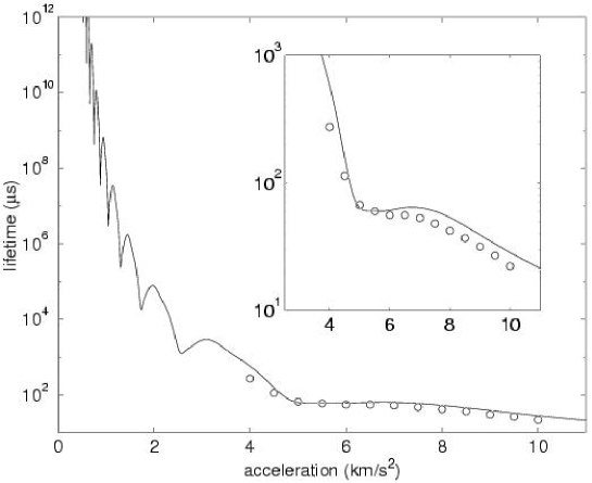
Figure 3.5: Lifetime of the ground Wannier state as a function of the external field. The solid line is the theoretical prediction, the circles are the experimental data of Ref. [124]. The insert blows up the interval $4000m/s^{2}<a<10000m/s^{2}$ considered in the cited experiment.

The lifetime of the Wannier-Stark states (given by $\tau=\hbar/\Gamma_{\alpha}$) as the function of static force was measured in an experiment with cold sodium atoms in a laser field [124]. The setting of the experiment [124] yields the accelerated cosine potential (the inertial force takes the role of the static field) and an effective Planck constant $\hbar=1.671$. For this value of the Planck constant one has only one under-barrier resonance, and the two-ladder model of Sec. 3.2 is already a good approximation of the real situation. Figure 3.5 compares the experimental results for the lifetime of the ground Wannier-Stark states with the theoretical results. The axes are adjusted to the experimental parameters. Namely, the field strength in our description is related to the acceleration in the experiment by the formula $F\approx 0.0383a$, where $a$ is measured in $km/s^{2}$, and the unit of time in our description is approximately $1.34\mu s$. The experimental data follow closely the theoretical curve. (Explicitly, the analytical form of the displayed dependence is given by Eq. (3.4) with $\epsilon=a\exp(-b/F)$, $a=1.0$, $b=0.254$.) In particular we note that the theory predicts a local minimum of the lifetime at $a=5000m/s^{2}$, which corresponds to the crossing of the ground and the first excited Wannier levels in neighboring wells. Unfortunately, the experimental data do not extend to smaller accelerations, where the theory predicts much stronger oscillations of the lifetime.

3.4 Wannier-Stark ladders in semiconductor superlattices

We proceed with the semiconductor superlattices. As mentioned in Sec. 1.4, the semiconductor superlattices are often modeled by the square-box potential (1.18), where $a$ and $b=d-a$ are the thickness of the alternating semiconductor layers. For the square-box potential (1.18) the width of the band gaps decreases only inversely proportional to the gap’s number. Because of this, one is forced to deal with infinite number of interacting Wannier-Stark ladders. However, as was argued in Ref. [163], this is actually an over-complication of the real situation. Indeed, the potential (1.18) is only a first approximation for the superlattice potential, which should be a smooth function of $x$. This fact can be taken into account by smoothing the rectangular step in (1.18) as

$$V(x)=\tanh\sigma(x+a\pi/2d)-\tanh\sigma(x-a\pi/2d)-1$$ (3.8)

for example. (Here we use scaled variables, where the potential is $2\pi$-periodic and $|V(x)|\leq 1$.) The parameter $\sigma^{-1}$ defines the size of the transition region between the semiconductor layers and, in natural units, it cannot be smaller than the atomic distance. The smoothing introduces a cut-off in the energy, above which the gaps between the Bloch bands decrease exponentially. Thus, instead of an infinite number of ladders associated with the above-barrier resonances, we may consider a finite number of them. The interaction of a large number of ladders originating from the high-energy Bloch bands was studied in some details in Ref. [163]. It was found that they typically form pairs of locked [in the sense of Eq. (3.6)] ladders which show anticrossings with each other.

Since the lifetime of the above-barrier resonances is much shorter than the lifetime of the under-barrier resonances one might imagine that the former are of minor physical importance. Although this is partially true, the above-barrier resonances cannot be ignored because they strongly affect the lifetime of the long-lived under-barrier resonances. This is illustrated in Fig. 3.6, where the resonance structure of the Wannier-Stark Hamiltonian with a periodic potential given by Eq. (3.8) and $\hbar=3.28$ is depicted as a gray-scaled map of the Wigner delay time (2.30). In terms of Fig. 3.1, this way of presentation of the numerical results means that each line in the lower panel has a “finite width” defined by the value $\Gamma$ in the upper panel. In fact, asssuming a Wigner relation [199] we get

$$\tau(E)=\tau_{0}+\sum_{\alpha}\left(\sum_{l=-\infty}^{\infty}{\rm Im}\left[\frac{\hbar}{\mathcal{E}_{\alpha}+2\pi Fl-E}\right]\right)\;,$$ (3.9)

where each term in the sum over $\alpha$ is just a periodic sequence of Lorentzians with width $\Gamma_{\alpha}$. (We recall that, by definition, $\tau(E)$ is a periodic function of the energy.) In the case of a large number of interacting ladders (i.e. in the case currently considered here, where more than 10 above-barrier resonances contribute to the sum over $\alpha$) we find this presentation more convenient because it reveals only narrow resonances, while the wide resonances contribute to the background compensated by the constant $\tau_{0}$. For the chosen value of the scaled Planck constant, $\hbar=3.28$, the periodic potential (3.8) supports only one under-barrier resonance, seen in the figure as a broken line going from the upper-left to the lower-right corners. Wide above-barrier resonances originating from the second and third Bloch bands and showing anticrossings with the ground resonance can be still identified, but the other resonances are indistinguishable because of their large widths. Nevertheless, the existence of these resonances is confirmed indirectly by the complicated structure of the “visible lines”.

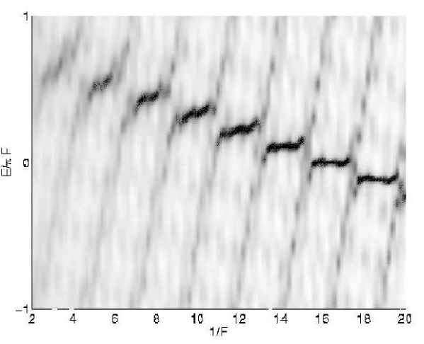
Figure 3.6: Grey-scaled map of the Wigner delay time (3.9) for the smoothed square-box potential (3.8). The parameters are $\hbar=3.28$, $a/b=39/76$ and $\delta=0.25$.

In conclusion, in comparison with the optical lattices, the structure of the Wannier-Stark resonances in semiconductor superlattices is complicated by the presence of large number of above-barrier resonances. Besides this, in the semiconductor superlattices a strong interaction between the ladders is the rule, while the case of weakly interacting ladders is typical for optical lattices.

Chapter 4 Spectroscopy of Wannier-Stark ladders

In this chapter we discuss the spectroscopy of Wannier-Stark ladders in optical and semiconductor superlattices. We show how the different spectroscopic quantities (measured in a laboratory experiment) can be directly calculated by using the formalism of the resonance Wannier-Stark states.

4.1 Decay spectrum and Fermi’s golden rule

The spectroscopy approach assumes that one probes a quantum system by a weak ac field $F_{\omega}x\cos(\omega t)$ with tunable frequency $\omega$. In our case, the system consists of different Wannier-Stark ladders of resonances, the two most stable of which are schematically depicted in Fig. 4.1. The driving induces transitions between the ground and the excited states. Scanning the frequency $\omega$ sequentially activates the different transition paths and the different Wannier states of the excited ladder are populated. Because the excited states are typically short-lived, they decay before the driving can transfer the population back to the ground state, i.e. before a Rabi oscillation is performed. Then the decay rate of the ground state is determined by the transition rate $D(\omega$) to the excited Wannier-Stark ladder. The width is written as

$$\Gamma_{0}(\omega)=\Gamma_{0}+D(\omega)\;,$$ (4.1)

where $\Gamma_{0}$ takes into account the decay in the absence of driving. In what follows we shall refer to the quantity $\Gamma_{0}(\omega)$ as the induced decay rate or the decay spectrum. In Sec. 5 we calculate the induced decay rate rigorously by using the formalism of quasienergy Wannier-Stark states. It will be shown that the decay spectrum is given by

$$\Gamma_{0}(\omega)=\Gamma_{0}+\frac{F^{2}_{\omega}}{2}\sum_{\beta>0}\sum_{L}{\rm Im}\left[\frac{V_{0,\beta}^{2}(L)}{(E_{\beta,l}+2\pi FL-E_{0,l}-\hbar\omega)-{\rm i}\Gamma_{\beta}/2}\right]\;,$$ (4.2)

where $F_{\omega}$ and $\omega$ are the amplitude and frequency of the probing field and

$$V_{0,\beta}^{2}(L)=\langle\Psi_{0,l}|x|\Psi_{\beta,l+L}\rangle\langle\Psi_{\beta,l+L}|x|\Psi_{0,l}\rangle$$ (4.3)

is the square of the dipole matrix element between an arbitrary ground Wannier-Stark state $\Psi_{0,l}(x)$ and the upper Wannier-Stark state $\Psi_{\beta,l+L}(x)$ shifted by $L$ lattice periods. We would like to stress that, because for the resonance wave functions $\langle\Psi_{\alpha,l}|x|\Psi_{\beta,l^{\prime}}\rangle\neq\langle\Psi_{\beta,l^{\prime}}|x|\Psi_{\alpha,l}\rangle^{*}$, the square of the dipole matrix element $V^{2}_{0,\beta}(L)$ is generally a complex number.

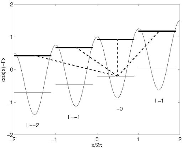
Figure 4.1: Schematic illustration of the transitions induced by a periodic driving. The positions of the ground and the first excited Wannier-Stark ladder are shown for $F=0.04$ and $\hbar=1.5$. The width of the states is symbolized by the different strength of the lines.

To understand the physical meaning of Eq. (4.2), it is useful to discuss its relation to Fermi’s golden rule, which reads

$$D(\omega)\approx\pi F^{2}_{\omega}\int{\rm d}E\,\Big{|}\int{\rm d}x\Psi^{*}_{E}(x)x\Psi_{E_{0,l}}(x)\Big{|}^{2}\rho(E)\delta(E-E_{0,l}-\hbar\omega)\;.$$ (4.4)

in the notations used. In Eq. (4.4), the $\Psi_{E}(x)$ are the hermitian eigenfunctions of the Hamiltonian (2.2) (i.e., $E$ is real and continuous) and $\rho(E)$ is the density of states. For the sake of simplicity we also approximate the ground Wannier-Stark resonance by the discrete level $E_{0,l}$. Then Eq. (4.4) describes the decay of a discrete level into the continuum. Assuming, for a moment, that the continuum is dominated by the first excited Wannier-Stark ladder, the density of states $\rho(E)$ is given by a periodic sequence of Lorentzians with width $\Gamma_{1}$, i.e.

$$\rho(E)\approx\frac{1}{2\pi}\sum_{L}\frac{\Gamma_{1}}{(E-E_{1,l+L})^{2}+\Gamma_{1}^{2}/4}\,.$$ (4.5)

Substituting the last equation into Eq. (4.4) and integrating over $E$ we have

$$D(\omega)\approx\frac{F^{2}_{\omega}}{2}\,\Big{|}\int{\rm d}x\Psi^{*}_{E_{0,l}+\hbar\omega}(x)x\Psi_{E_{0,l}}(x)\Big{|}^{2}\sum_{L}\frac{\Gamma_{1}}{(E_{1,l+L}-E_{0,l}-\hbar\omega)^{2}+\Gamma_{1}^{2}/4}\;.$$ (4.6)

In the case $\Gamma_{1}\ll 2\pi F$ the Lorentzians in the right-hand side of Eq. (4.6) are $\delta$-like functions of the argument $\hbar\omega=E_{1,l}+2\pi FL-E_{0,l}$. Thus the transition matrix element can be moved under the summation sign, which gives

$$D(\omega)\approx\frac{F^{2}_{\omega}}{2}\sum_{\beta>0}\sum_{L}|\widetilde{V}_{0,\beta}|^{2}(L)\frac{\Gamma_{\beta}}{(E_{\beta,l}+2\pi FL-E_{0,l}-\hbar\omega)^{2}+\Gamma_{\beta}^{2}/4}\;,$$ (4.7)

where

$$|\widetilde{V}_{0,\beta}|^{2}(L)=\Big{|}\int{\rm d}x\Psi^{*}_{E_{\beta,l+L}}(x)x\Psi_{E_{0,l}}(x)\Big{|}^{2}$$ (4.8)

(here we again included the possibility of transitions to the higher Wannier ladders, which is indicated by the sum over $\beta$). It is seen that that the obtained result coincides with Eq. (4.2) if the coefficients $|\widetilde{V}_{0,\beta}|^{2}(L)$ are identified with the squared dipole matrix elements (4.3). Obviously, this holds in the limit $F\rightarrow 0$, when the resonance wave functions can be approximated by the localized states. For a strong field, however, Eq. (4.7) is a rather poor approximation of the decay spectrum. In particular, it is unable to predict the non-Lorentzian shape of the lines, which is observed in the laboratory and numerical experiments and which is correctly captured in Eq. (4.2) by the complex phase of the squared dipole matrix elements $V_{0,\beta}^{2}(L)$.

To proceed further, we have to calculate the squared matrix elements (4.3). A rough estimate for $V_{0,\beta}^{2}(L)$ can be obtained on the basis of Eq. (1.11), which approximates the resonance Wannier-Stark state by the sum of the localized Wannier states: $\Psi_{\alpha,l}=\sum_{m}J_{m-l}(\Delta_{\alpha}/4\pi F)\psi_{\alpha,m}$. The typical experimental settings (see Sec. 4.3) correspond to $\Delta_{0}/4\pi F\ll 1$ and $\Delta_{\beta}/4\pi F>1$. Then the values of the matrix elements are approximately

$$V_{0,\beta}^{2}(L)\approx|\widetilde{V}_{0,\beta}|^{2}(L)\approx|\langle\psi_{0,l}|x|\psi_{\beta,l}\rangle|^{2}J^{2}_{L}\left(\frac{\Delta_{\beta}}{4\pi F}\right)\;,$$ (4.9)

which contribute mainly in the region $L<\Delta_{\beta}/4\pi F$, the localization length of the excited Wannier-Stark states. The degree of validity of this result is discussed in the next subsection.

4.2 Dipole matrix elements

In this subsection we calculate the dipole matrix elements

$$V_{\alpha,\beta}(l-l^{\prime})=\langle\Psi_{\alpha,l}|x|\Psi_{\beta,l^{\prime}}\rangle$$ (4.10)

beyond the tight-binding approximation. We shall use Eq. (2.40)

$$\Psi_{\alpha,l}(x)=\int{\rm d}\kappa\,{\rm e}^{-{\rm i}2\pi l\kappa}\Phi_{\alpha,\kappa}(x)\;,\quad\Phi_{\alpha,\kappa}(x)={\rm e}^{{\rm i}\kappa x}\chi_{\alpha,\kappa}(x)\;,\quad\chi_{\alpha,\kappa}(x)=\chi_{\alpha,\kappa}(x+2\pi)\;,$$ (4.11)

which relates the Wannier-Stark states $\Psi_{\alpha,l}(x)$ to the Wannier-Bloch states $\Phi_{\alpha,\kappa}(x)$. As follows from the results of Sec. 2, the function $\chi_{\alpha,\kappa}(x)$ can be generated from $\chi_{\alpha,0}(x)$ by propagating it in time

$$|\chi_{\alpha,\kappa}\rangle=\exp\left({\rm i}\,\frac{\mathcal{E}_{\alpha}t}{\hbar}\right)\widetilde{U}(t)|\chi_{\alpha,0}\rangle\;,$$ (4.12)

where $\widetilde{U}(t)$ is the continuous version of the operator $\widetilde{U}$ defined in Eq. (2.11) and the quasimomentum $\kappa$ is related to time $t$ by $\kappa=-Ft/\hbar$. Substituting Eq. (4.11) and Eq. (4.12) into Eq. (4.10) we obtain the dipole matrix elements as the Fourier image

$$V_{\alpha,\beta}(l-l^{\prime})=2\pi l\,\delta_{\alpha,\beta}^{l,l^{\prime}}+\int{\rm d}\kappa\,{\rm e}^{{\rm i}2\pi(l-l^{\prime})\kappa}X_{\alpha,\beta}(\kappa)$$ (4.13)

of the periodic function

$$X_{\alpha,\beta}(\kappa)={\rm i}\,\langle\chi_{\alpha,\kappa}|\,\frac{\partial}{\partial\kappa}\chi_{\beta,\kappa}\rangle=\frac{1}{F}\,\langle\chi_{\alpha,\kappa}|\,\frac{(p+\hbar\kappa)^{2}}{2}+V(x)\,|\chi_{\beta,\kappa}\rangle-\frac{\mathcal{E}_{\alpha}}{F}\,\delta_{\alpha,\beta}\;.$$ (4.14)

The last two equations provide the basis for numerical calculation of the transition matrix elements. We also recall that one actually needs the square of the matrix elements (4.3) but not the matrix elements themselves (which are defined up to an arbitrary phase). Thus we first calculate $V_{\alpha,\beta}(L)$ and $V_{\beta,\alpha}(L)$ for $L=0,\pm 1,\ldots$ and then multiply them term by term.

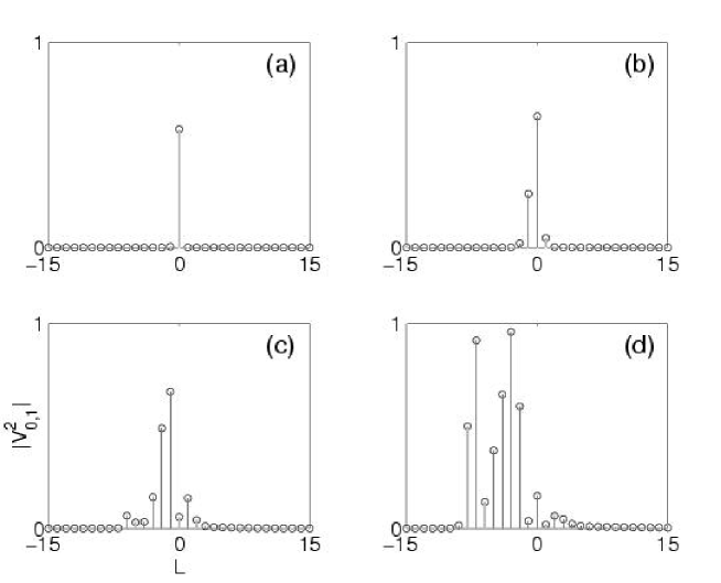
Figure 4.2: The absolute values of the squared dipole matrix elements (4.3) for $V(x)=\cos x$, $F=0.04$ and $\hbar=1$ (a), $1.5$ (b), $2$ (c), and $2.5$ (d).

In Fig. 4.2 we depict the squared dipole matrix elements between the ground and first excited Wannier-Stark states for $V(x)=\cos x$, a moderate values of the static force $F=0.04$ and values of the scaled Planck constant in the interval $1\leq\hbar\leq 2.5$. For $\hbar=1.0$ the Bloch bands width $\Delta_{1}\approx 0.05$ is much smaller than $4\pi F\approx 0.5$ and the upper Wannier-Stark state is essentially localized within single potential well. Then only “vertical” transitions, $L=0$, are possible between the ground and first excited Wannier ladders. By increasing $\hbar$ the localization length of the upper state grows (proportional to the band width) and more than one matrix element may differ from zero. Simultaneously, the Wannier levels move towards the top of the potential barrier (for $\hbar>1.6$ the upper Wannier level is already above the potential barrier) and the Wannier state looses its stability ($\Gamma_{1}=1.90\cdot 10^{-15}$, $1.35\cdot 10^{-2}$, $5.24\cdot 10^{-2}$, and $1.14\cdot 10^{-1}$, for $\hbar=1$, 1.5, 2, and 2.5). Because for short-lived resonances the tight-binding result (1.11) is a rather poor approximation of the resonance wave functions, we observe an essential deviation from Eq. (4.9). In particular we note a strong asymmetry of the matrix elements with respect to $L$. It appears that the transitions “down the ladder” are enhanced in comparison with the transitions “up the ladder”. At the same time, for weak far transitions ($L\gg 1$) the situation is reversed [see Fig. 4.2(d) and Fig. 4.4(b) below].

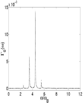
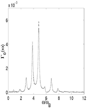
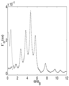
Figure 4.3: Comparison of the $\omega$-dependence in (4.2) (solid line) with the exact numerical calculation of the induced decay rate (dashed line). Parameters are $F=0.04$, $F_{\omega}=0.02$ and $\hbar=1.5$ (left), $\hbar=2.0$ (middle) and $\hbar=2.5$ (right panel).

Substituting the calculated matrix elements into Eq. (4.2), we find the decay spectra of the system. The solid line in Fig. 4.3 shows the decay spectra for $\hbar=1.5$, 2.0, 2.5. As expected, $\Gamma_{0}(\omega)$ has number of peaks with the same width $\Gamma_{1}$ separated by the Bloch frequency $\omega_{B}$. The relative heights of the peaks are obviously given by the absolute values of the squared dipole matrix elements shown in Fig. 4.2, while the shape of the lines is defined by the phase of $V_{0,\beta}^{2}(L)$. As mentioned above, the phases of the squared dipole matrix elements are generally not zero and, therefore, the shape of the lines is generally non-Lorentzian. In other words, we meet the case of Fano-like resonances [172]. For the sake of comparison the dashed lines in Fig. 4.3 show the results of an exact numerical calculation of the decay rate. A good correspondence is noticed. The discrepancy in the region of small driving frequency is due to the rotating wave approximation (which is implicitly assumed in the Fermi golden rule) and the effect of the diagonal matrix elements $V_{\alpha,\alpha}^{2}(L)$ (which are also ignored in the Fermi golden rule approach). In principle, the region of small driving frequency requires a separate analysis.

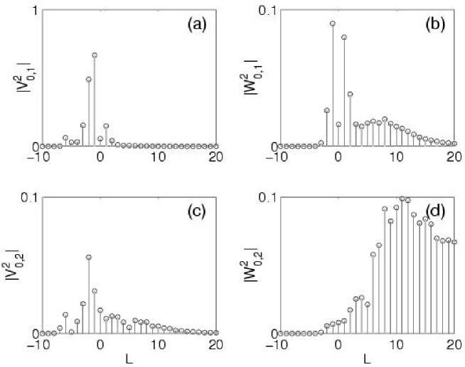
Figure 4.4: The absolute values of the transition coefficients $V_{0,1}^{2}(L)$ (a), $W_{0,1}^{2}(L)$ (b), $V_{0,2}^{2}(L)$ (c), and $W_{0,2}^{2}(L)$ (d).

In conclusion, we discuss the effect of direct transitions to the second excited Wannier ladder. For the case $\hbar=2$ the squared dipole matrix elements $V_{0,1}^{2}(L)$ and $V_{0,2}^{2}(L)$ are compared in the left column of Fig. 4.4. It is seen that the main lines in Fig. 4.4(c) are ten times smaller than those in Fig. 4.4(a). Thus the effect of higher transitions can be neglected. We note, however, that this is not always the case. In the next section we consider a situation when the direct transitions to the second excited Wannier ladder can not be ignored.

4.3 Decay spectra for atoms in optical lattices

The induced decay rate $\Gamma_{0}(\omega)$ was measured for the system of cold atoms in the accelerated standing laser wave [123, 125]. Because the atoms are neutral, the periodic driving of the system was realized by means of a phase modulation of the periodic potential:

$$H=\frac{p^{2}}{2}+\cos[x+\varepsilon\cos(\omega t)]+Fx\;,$$ (4.15)

Using the Kramers-Henneberger transformation [173, 174, 175, 176] the Hamiltonian (4.15) can be presented in the form

$$H=\frac{p^{2}}{2}+\cos(x)+Fx+F_{\omega}x\cos(\omega t)\;,\quad F_{\omega}=\varepsilon\omega^{2}\;.$$ (4.16)

Thus, the phase modulation is equivalent to the effect of an ac field. Considering the limit of small $\varepsilon$, where $\cos[x+\varepsilon\cos(\omega t)]\approx\cos x+\varepsilon\sin x\cos(\omega t)$, we can adopt Eq. (4.2) of the previous section to cover the the case of phase modulation. Namely, the amplitude $F_{\omega}$ in Eq. (4.2) should be substituted by $\varepsilon$ and the squared dipole matrix elements (4.3) by the squared matrix elements

$$W_{0,\beta}^{2}(L)=\langle\Psi_{0,l}|\sin x|\Psi_{\beta,l+L}\rangle\langle\Psi_{\beta,l+L}|\sin x|\Psi_{0,l}\rangle\;.$$ (4.17)

Moreover, according to the commutator relation for the Hamiltonian of the non-driven system

$$\hbar^{-2}[H_{W},[H_{W},x]]=-\sin x+F\;,$$ (4.18)

the squared matrix elements $W_{0,\beta}^{2}(L)$ are related to the squared dipole matrix elements $V_{0,\beta}^{2}(L)$ by

$$W^{2}_{0,\beta}(L)=\left|\frac{\mathcal{E}_{\beta,l+L}-\mathcal{E}_{0,l}}{\hbar}\right|^{4}\,V^{2}_{0,\beta}(L)\;.$$ (4.19)

It follows from the last equation that the way of driving realized in the optical lattices suppresses the transition down the ladder and enhances the transition up the ladder. This is illustrated in Fig. 4.4, where we compare the squared matrix elements $W^{2}_{0,\beta}(L)$ and $V^{2}_{0,\beta}(L)$ for $\beta=1,2$ calculated on the basis of Eq. (4.17) and Eq. (4.3), respectively. It is seen that the practically invisible tail of far transitions in Fig. 4.4(a) shows up in Fig. 4.4(b). Besides this, for $L\gg 1$ the squared matrix elements between the ground and second excited Wannier-Stark states are larger than those between the ground and first excited one. Because the width of the second excited Wannier-Stark resonance $\Gamma_{2}$ is lager than $\Gamma_{1}$ (and actually larger than the Bloch energy), the transition to the first and second excited Wannier ladders may interfere. Indeed, this is the case usually observed in the high-frequency regime of driving (see Fig. 4.5, which should be compared with Fig. 4.3).

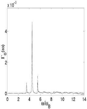
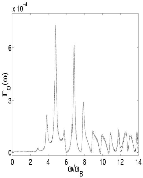
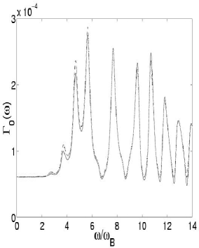
Figure 4.5: Decay spectra as a function of the driving frequency $\omega$. Parameters are $F=0.04$, $\varepsilon=0.02$ and $\hbar=1.5$ (left), $\hbar=2.0$ (middle) $\hbar=2.5$ (right panel). The exact numerical calculation (dashed lines) are compared to the model prediction (solid lines). Note a complicated structure of the decay spectra in the high-frequency region caused by the interference of the transitions to the first and second excited Wannier-Stark ladders.

We proceed with the experimental data for the spectroscopy of atomic Wannier-Stark ladders [123] (note also the improved experiment [125]). The setup in the experiment [123] is as follows. Sodium atoms were cooled and trapped in a far-detuned optical lattice. Then, introducing a time-dependent phase difference between the two laser beams forming the lattice, the lattice was accelerated (see Sec. 1.4). After some time, only atoms in the ground Wannier-Stark states survived, i.e. a superposition of ground ladder Wannier-Stark states was prepared. Then an additional phase driving of frequency $\omega$ was switched on and the survival probability,

$$P_{t}(\omega)=\exp\left(-\frac{\Gamma_{0}(\omega)t}{\hbar}\right)\;,$$ (4.20)

was measured. The experiment was repeated for different values of $\omega$. In scaled units the experimental settings with $V_{0}/h=75\pm 7kHz$ (we choose the value $V_{0}/h=68kHz$, which is used in all numerical simulations in [123]) and $a=1570m/s^{2}$ correspond to $\hbar=1.709$ and $F=0.0628$. (For these parameters the ground and first excited state have the widths $\Gamma_{0}=2.38\cdot 10^{-5}$ and $\Gamma_{1}=6.11\cdot 10^{-2}$, respectively.) The timescale in the experiments is $1.37\mu s$, and the Bloch frequency is $\omega_{B}/2\pi=26.85kHz$. The driving amplitude was $\varepsilon=0.096$. The left panel of Fig. 4.6 shows the decay spectra as a function of the frequency in this case. The vertical transition dominates the figure, accompanied by the two transitions with $L=\pm 1$ and a tail of transitions with positive $L\gg 1$. In the right panel, the experimental data for the survival probability $P_{t}(\omega)$ are compared to our numerical data. The time $t$ is taken as an adjustable parameter and chosen such that the depth of the peaks approximately coincide. The curve shows the survival probability at $t=300\mu s$ corresponding to $t=219$ in scaled units. A good correspondence between experiment and theory is noticed. The minima of the survival probability appear when the driving frequency fits to a transition. The relative depth of the minima reflecting the size of the transition matrix elements agrees reasonably. Furthermore, the asymmetric shape of the minimum between $4\omega_{B}$ and $5\omega_{B}$ is reproduced. Note that the experimental data also allow to extract the width of the first excited state from the width of the central minimum: $\Gamma_{1}\approx 0.3\omega_{B}\approx 6.9\cdot 10^{-2}$, which is in reasonable agreement with the numerical result $\Gamma_{1}=6.11\cdot 10^{-2}$.

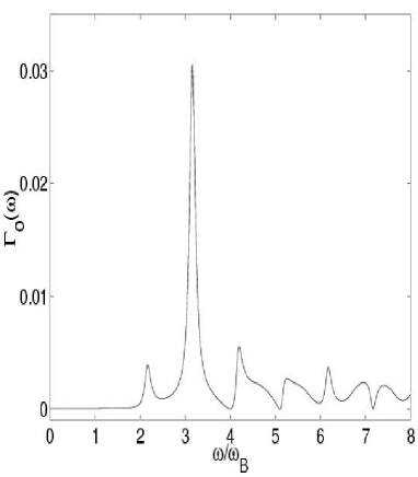
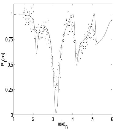
Figure 4.6: The left panel shows the induced decay rate of the ground Wannier-Stark state as function of the driving frequency for $\hbar=1.709$, $F=0.0628$ and $\varepsilon=0.096$. The right panel compares the experimental data from [123] with the calculated survival probability $P_{t}(\omega)$ for $t=300\mu s$.

4.4 Absorption spectra of semiconductor superlattices

Equation (4.2) of Sec. 4.1 can be generalized to describe the absorption spectrum $D(\omega)$ of undoped semiconductor superlattices [163]. This generalization has the form

$$D(\omega)\sim\sum_{\alpha,\beta}\sum_{L}{\rm Im}\left[\frac{I_{\alpha,\beta}^{2}(L)}{(E_{\beta,l}^{e}-E_{\alpha,l}^{h}+edFL+E_{g}-\hbar\omega)-{\rm i}(\Gamma_{\beta}^{e}+\Gamma_{\alpha}^{h})/2}\right]\;,$$ (4.21)

where the upper indices $e$ and $h$ refer to the electron and hole Wannier-Stark states, respectively, $E_{g}$ is the energy gap between the conductance and valence bands in the bulk semiconductor, and

$$I_{\alpha,\,\beta}^{2}(L)=\langle\Psi_{\alpha,\,l}^{h}|\Psi_{\beta,\,l+L}^{e}\rangle\langle\Psi_{\beta,\,l+L}^{e}|\Psi_{\alpha,\,l}^{h}\rangle$$ (4.22)

is the square of the overlap integral between the hole and electron wave functions. Repeating the arguments of Sec. 4.1 it is easy to show that in the low-field limit Eq. (4.21) is essentially the same as the Fermi golden rule equation

$$D(\omega)\sim\int\int{\rm d}E^{e}{\rm d}E^{h}\Big{|}\int{\rm d}x\Psi^{e}(x;E^{e})\Psi^{h}(x;E^{h})\Big{|}^{2}\rho^{e}(E^{e})\rho^{h}(E^{h})\delta(E^{e}-E^{h}+E_{g}-\hbar\omega)\;,$$ (4.23)

where $\rho^{e}(E^{e})$ and $\rho^{h}(E^{h})$ are the one-dimensional electron and hole densities of states. According to Ref. [47, 121] the quantity $D(\omega)$, which can be interpreted as the probability of creating the electron-hole pair by a photon of energy $\hbar\omega$ (the electron-hole Coulomb interaction is neglected), is directly related to the absorption spectrum of the semiconductor superlattices measured in the laboratory experiments.

It follows from Eq. (4.21) that the structure of the absorption spectrum depends on the values of the squared overlap integral Eq. (4.22) which, in turn, depend on the value of the static field. In the low-field regime the Wannier-Stark states are delocalized over several superlattice periods and many transition coefficients $I_{\alpha,\,\beta}^{2}(L)$ differ from zero. In the high-field regime the Wannier-Stark states tend to be localized within a single well and the vertical transitions $L=0$ become dominant. We would like to stress, however, that the process of localization of the Wannier-Stark states is always accompanied by a loss of their stability. As mentioned above, the latter process restricts the validity of the tight-binding results concerning a complete localization of the Wannier-Stark states in the limit of strong static field.

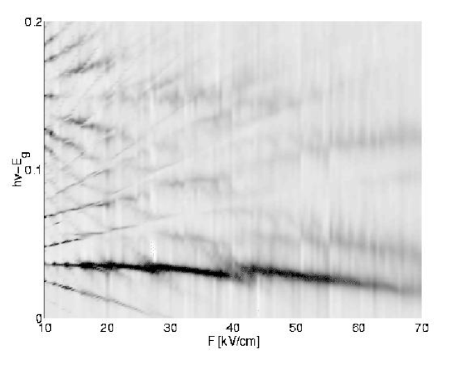
Figure 4.7: Grey-scaled map of the one-dimensional absorption spectra (4.21) as a function of the static field $F$ and photon energy $h\nu$.

As an illustration to Eq. (4.22), Fig. 4.7 shows the absorption spectrum of the semiconductor superlattice studied in the experiment [121]. (This should be compared with the absorption spectrum calculated in Ref. [47] by using a kind of finite-box quantization method.) The depicted result is a typical example of a Wannier-Stark fan diagram. By close inspection of the figure one can identify at least four different fans associated with the transitions between $\alpha=0,1$ hole and $\beta=0,1$ electron states. However, in the region of strong static fields considered here, the majority of these transitions are weak and the whole spectrum is dominated by the vertical $L=0$ transition between the ground hole and electron states. Note a complicated structure of the main line resembling a broken feather. Recalling the results of Sec. 3.4 (see Fig. 3.6), this structure originates from avoided crossings between the (ground) under-barrier and (first) above-barrier electron resonances. Such a “broken feather” structure was well observed in the cited experiment [121].

Chapter 5 Quasienergy Wannier-Stark states

In the following chapters we investigate Wannier-Stark ladders in combined ac and dc fields. Then the Hamiltonian of the system is

$$H=\frac{p^{2}}{2}+V(x)+Fx+F_{\omega}x\cos(\omega t)\,,$$ (5.1)

or, as described in Sec. 4.3, equivalently given by

$$H=\frac{p^{2}}{2}+V[x+\varepsilon\cos(\omega t)]+Fx\,,\quad\varepsilon=F_{\omega}/\omega^{2}\;.$$ (5.2)

Depending on the particular analytical approach we shall use either of these two forms. Let us also note that the Hamiltonian (5.2) can be generalized to include the case of arbitrary space- and time-periodic potential $V(x,t)=V(x+2\pi,t)=V(x,t+T_{\omega})$.

5.1 Single-band quasienergy spectrum

For time-dependent potentials the period of the potential sets an additional time scale. In order to define a Floquet-Bloch operator with properties similar to the time-independent case, we have the restriction that the period $T_{\omega}$ of the potential and the Bloch time $T_{B}$ are commensurate, i.e.

$$pT_{\omega}=qT_{B}\equiv T\;.$$ (5.3)

In this case the Floquet operator $U(T)$ over the common period $T$ can be presented as

$$U(T)={\rm e}^{-{\rm i}qx}\,\widetilde{U}(T)\;,\quad\widetilde{U}(T)=\widehat{\exp}\left(-\frac{{\rm i}}{\hbar}\int_{0}^{T}{\rm d}t\,\left[\frac{(p-Ft)^{2}}{2}+V(x,t)\right]\right)\;,$$ (5.4)

(compare with Eqs. (2.10)–(2.11)). Consequently the eigenstates of $U(T)$,

$$U(T)\,\Phi(x;\lambda,\kappa)=\lambda\Phi(x;\lambda,\kappa)\;,\quad\lambda=\exp(-{\rm i}ET/\hbar)\;,$$ (5.5)

can be chosen to be the Bloch-like states [177, 178], i.e. $\Phi(x+2\pi;\lambda,\kappa)=e^{{\rm i}2\pi\kappa}\Phi(x;\lambda,\kappa)$. Due to the time-periodicity of the potential, $V(x,t+T_{\omega})=V(x,t)$, we have the relation

$$U(T)=U(T_{\omega})^{p}=\left[\exp(-{\rm i}\,x\,q/p)\,\widetilde{U}(T_{\omega})\right]^{p}\;.$$ (5.6)

As a direct consequence of this relation, the states $\Phi(x;\lambda,\kappa)$ with the quasimomentum $\kappa-r/p$ ($r=0,1,\dots,p-1$) are Floquet states with the same quasienergy. In terms of the operator $U^{(\kappa)}(T)=\exp(-{\rm i}\kappa x)U(T)\exp({\rm i}\kappa x)$ this means that the operators $U^{(\kappa)}(T)$ are unitarily equivalent for these values of the quasimomentum. Therefore, the Brillouin zone of the Floquet operator $U(T)$ is $p$-fold degenerate. In the next section we introduce the resonance Wannier-Bloch functions $\Phi_{\alpha,\kappa}(x)$ which satisfy the eigenvalue equation (5.5) with the Siegert (i.e. purely outgoing wave) boundary condition and correspond to the complex energy $\mathcal{E}_{\alpha}(\kappa)$. Then the $p$-fold degeneracy of the Brillouin zone just means that the dispersion relation $\mathcal{E}_{\alpha}(\kappa)$ is a periodic function of the quasimomentum with period given by $p$.

It should be noted that the Wannier-Bloch functions $\Phi(x;\lambda,\kappa)$ (hermitian boundary condition) or $\Phi_{\alpha,\kappa}(x)$ (Siegert boundary condition) are not the quasienergy functions of the system because the latter, by definition, are the eigenfunctions of the evolution operator $U(T_{\omega})$ over the period of the driving force. However, the quasienergy functions can be expressed in terms of the Wannier-Bloch functions as

$$\Psi_{\alpha,\kappa}^{(n)}(x)=\frac{1}{p}\sum_{r=0}^{p-1}\exp\left[-{\rm i}\,\frac{2\pi n}{p}r\right]\Phi_{\alpha,\kappa+r/p}(x)\,.$$ (5.7)

Equation (5.7) is the discrete analogue of the relation (2.40) between the Wannier-Bloch and Wannier-Stark states in the case of pure dc field. Since the evolution operator $U(T_{\omega})$ commutes with the translational operator over $p$ lattice periods, the quasienergy states $\Psi_{\alpha,\kappa}^{(n)}(x)$ are the eigenfunctions of this shift operator. In particular, as easily deduced from Eq. (5.7), in the limit $\varepsilon\rightarrow 0$ the function $\Psi_{\alpha,\kappa}^{(n)}(x)$ is a linear combination of every $p$-th state of the Wannier-Stark ladder (and altogether there are $p$ different subladders). Thus, as well as the Wannier-Bloch states $\Phi_{\alpha,\kappa}(x)$, the eigenstates of $U(T_{\omega})$ are extended states. Note that the Brillouin zone is reduced now by a factor $p$, i.e the quasimomentum is restricted to $-1/2p\leq\kappa\leq 1/2p$. On the other hand, as $T_{\omega}=T/p$, the energy Brillouin zone is enlarged by this factor, i.e. the quasienergies take values in the interval $0\leq{\rm Re}\,\mathcal{E}\leq\hbar\omega$. Thus, if $\mathcal{E}_{\alpha}(\kappa)$ is the complex band of the Floquet operator (5.4), the complex quasienergies corresponding to the quasienergy states (5.7) are

$$\mathcal{E}^{(n)}_{\alpha}(\kappa)=\mathcal{E}_{\alpha}(\kappa)+\hbar\omega\,\frac{n}{p}\;,\quad\hbar\omega=2\pi F\,\frac{p}{q}\;.$$ (5.8)

In the remainder of this section we discuss the dispersion relation $\mathcal{E}_{\alpha}(\kappa)$ for the quasienergy bands on the basis of the single-band model. It is understood, however, that the single-band approach can describe at its best only the real part $E={\rm Re}\mathcal{E}$ of the spectrum.

In the single band analysis [54], it is convenient to work in the representation (5.1). Assuming that the two timescales are commensurate, the Houston functions (1.13) can be generalized to the Wannier-Bloch functions, which yields the following result for the quasienergy spectrum

$$E_{\alpha}(\kappa)=\frac{1}{T}\int_{0}^{T}\epsilon_{\alpha}(\kappa(t)\,)\,{\rm d}t\;,\quad\kappa(t)=\kappa-\frac{Ft}{\hbar}-\frac{F_{\omega}}{\hbar\omega}\,\sin(\omega t)\,,$$ (5.9)

In this equation, as before, $\epsilon_{\alpha}(\kappa)$ is the Bloch spectrum of the field-free Hamiltonian $H_{0}=p^{2}/2+V(x)$ and $\kappa(t)$ is the solution of the classical equation of motion for the quasimomentum with initial value $\kappa$. Expanding the Bloch dispersion relation into the Fourier series

$$\epsilon_{\alpha}(\kappa)=\sum_{\nu=0}^{\infty}\widetilde{\epsilon}_{\alpha}(\nu)\cos(2\pi\nu\kappa)$$ (5.10)

we obtain after some transformations

$$E_{\alpha}(\kappa)=\sum_{\mu=0}^{\infty}\,J_{\mu q}\Big{(}\frac{\mu qF_{\omega}}{F}\Big{)}\,\widetilde{\epsilon}_{\alpha}(\mu p)\cos(2\pi p\mu\kappa)\;.$$ (5.11)

Thus, the dispersion relation for the quasienergies is given by the original Bloch dispersion relation with rescaled Fourier coefficients. For the low-lying bands, the coefficients $\widetilde{\epsilon}_{\alpha}(\nu)$ rapidly decrease with $\nu$, and for practical purpose it is enough to keep only two first terms in the sum over $\mu$.

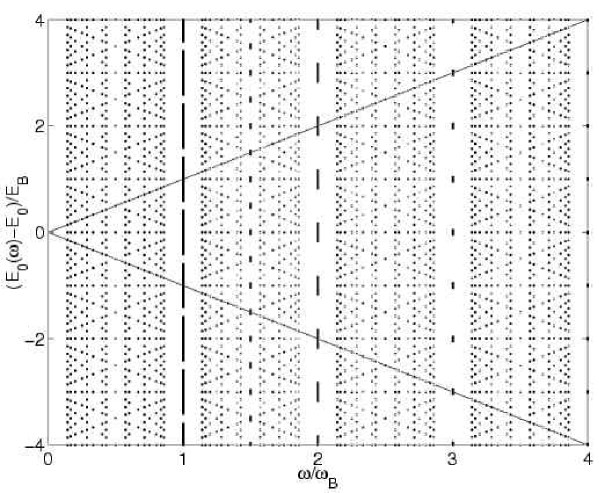
Figure 5.1: The band structure of the quasienergy spectrum originating from the ground ($\alpha=0$) Bloch band as predicted by the single-band model. The parameters of the non-driven system are $\hbar=3$, $F=0.08$ and the driving amplitude is $\varepsilon=1$. Only the rational values $\omega/\omega_{B}=p/q$ with $q\leq 7$ are considered. The straight lines restricts the interval $|E|\leq\hbar\omega$ corresponding to two (quasi)energy Brillouin zones.

Because the absolute value of the Bessel function is smaller than unity, the width of the quasienergy band is always smaller than the width of the parent Bloch band. In particular, assuming $\epsilon_{\alpha}(\kappa)\approx\bar{\epsilon}_{\alpha}+(\Delta_{\alpha}/2)\cos(2\pi\kappa)$ (as in the tight-binding approximation) and the simplest case of the resonant driving $\omega=\omega_{B}$ ($p=q=1$), we have

$$E_{\alpha}(\kappa)\approx\bar{\epsilon}_{\alpha}+J_{1}\Big{(}\frac{F_{\omega}}{F}\Big{)}\frac{\Delta_{\alpha}}{2}\,\cos(2\pi\kappa)\;.$$ (5.12)

As follows from this equation, the width of the quasienergy band approaches zero at zeros of the Bessel function $J_{1}(z)$. This phenomenon is often referred to in the literature as a dynamical band suppression in combined ac-dc fields [49, 50, 51, 52, 53, 54, 55, 56] . A similar behavior in the case of a pure ac field was predicted in [49, 55] and experimentally observed in [138].

Let us finally discuss the case of an irrational ratio of the Bloch and the driving frequency, $\gamma=\omega/\omega_{B}$. We can successively approximate the irrational $\gamma$ by rational numbers $p_{j}/q_{j}$, which are the $j$-th approximants of a continued fraction expansion of $\gamma$. Then, as for a typical $\gamma$ both $p_{j},q_{j}\rightarrow\infty$, the bandwidth of this approximation exponentially decreases to zero and the quasienergy spectrum turns into a discrete point spectrum [53]. This is illustrated by Fig. 5.1, where the band structure of the quasienergy spectrum (5.8), calculated on the basis of Eq. (5.11), is presented for $\alpha=0$ and constant value of driving amplitude $\varepsilon=F_{\omega}\omega^{2}$. (The parameters of the non-driven system with $V(x)=\cos x$ are $\hbar=3$ and $F=0.08$.) Note that the quasienergy bands have a noticeable width only for integer values of $p$.

It is an appropriate place here to note the similarity between the quasienergy spectrum of a driven Wannier-Stark system and the energy spectrum of a Bloch electron in a constant magnetic field. The latter is known to depend on the so-called magnetic matching ratio

$$\beta=\frac{eBd^{2}}{2\pi\hbar c}\;,$$ (5.13)

where $d$ is the lattice period. The spectrum of the ground state energies as a function of $\beta$ forms the famous Hofstadter butterfly [180]. In particular, for rational control parameter $\beta=p/q$ the number of distinct energy bands in the spectrum is given by the denominator $q$. Note that the magnetic matching ratio can be interpreted as ratio of two timescales, one of which is the time $d^{2}m/2\pi\hbar$ a particle with momentum $2\pi\hbar/d$ needs to cross the fundamental period $d$, and the other is the period $eB/mc$ of the cyclotron motion. Similar, the driven Wannier-Stark system has two intrinsic timescales and the structure of the quasienergy spectrum depends on the control parameter $\gamma=T_{B}/T_{\omega}=\hbar\omega/edF$, which is often referred to as the electric matching ratio.

5.2 S-matrix for time-dependent potentials

Provided the condition (5.3) is satisfied, the definition of a scattering matrix closely follows that of Sec. 2.2. Thus we begin with the matrix form of the eigenvalue equation (5.5), which reads

$$\sum_{n}\widetilde{U}^{(\kappa)}_{m+q,n}\,G_{S}(n)=\lambda\,G_{S}(m)\,.$$ (5.14)

(To simplify the formulas we shall omit the quasimomentum index in what follows.) Comparing this equation with Eq. (2.18), we note that index of the matrix $\widetilde{U}$ is now shifted by $q$. Because of this, we have $q$ different asymptotic solutions, which should be matched to each other. Using the terminology of the common scattering theory we shall call these solution the channels.

It is worth to stress the difference in the notion of decay channels introduced above and the notion of decay channels in the problem of above threshold ionization (a quantum particle in a single potential well subject to a time-periodic perturbation) [181]. In the latter case there is a well defined zero energy in the problem (e.g., a ground state of the system). Then the periodic driving originates a ladder of quasienergy resonances separated by quanta $\hbar\omega$ of the external field and, thus, the number of the corresponding decay channels is infinite. In the Wannier-Stark system, however, the ladder induced by the periodic driving (let us first discuss the simplest case $p=q=1$) coincides with the original Wannier-Stark ladder. In this sense the driving does not introduce new decay channels. These new channels appear only when the induced ladder does not coincide with the original ladder. Moreover, in the commensurate case $\omega/\omega_{B}=p/q$ (because of the partial coincidence of the ladders) their number remains finite. With this remark reserved we proceed further.

As before, we decompose the vector $G_{S}$ into three parts, i.e. $G_{S}^{(+)}$ contains all coefficients with $n>N$ and $G_{S}^{(-)}$ all coefficients with $n<-N-q$. The third part, $G_{S}^{(0)}$, contains all remaining coefficients with $-N-q\leq n\leq N$. The coefficients of $G_{S}^{(+)}$ and $G_{S}^{(-)}$ are defined recursively,

$$G_{S}(m)=(\lambda/u_{m})\,G_{S}(m-q) {\rm for}\,\,m>N\,,$$ (5.15)

$$G_{S}(m-q)=(u_{m}/\lambda)\,G_{S}(m) {\rm for}\,\,m<-N\,,$$ (5.16)

where $u_{m}=\exp({\rm i}\hbar^{2}[(\kappa+m-q)^{3}-(\kappa+m)^{3}]/6F)$. Let $W$ be the matrix $\widetilde{U}$ truncated to the size $(2N+1)\times(2N+1)$, and, furthermore, let $O_{m,n}$ be an $m\times n$ matrix of zeros. With the help of the definition

$$B_{N}=\left(\begin{array}[]{cc}O_{q,2N+1}&O_{q,q}\\[5.69054pt] W&O_{2N+1,q}\\ \end{array}\right)\;,$$ (5.19)

the equation for $G_{S}^{(0)}$ reads

$$(B_{N}-\lambda\leavevmode\hbox{\small 1\kern-3.8pt\normalsize 1})\,G_{S}^{(0)}=-\left(\begin{array}[]{c}u_{N+q}G_{S}(N+q)\\ \vdots\\ u_{N+1}G_{S}(N+1)\\[5.69054pt] O_{2N+1,1}\\ \end{array}\right)\;.$$ (5.24)

The right hand side of the last equation contains $q$ subsequent terms $G_{S}(m)$ and therefore contributions from the $q$ different incoming asymptotes. However, we can treat the different incoming channels separately, because the sum of solutions for different inhomogeneities yields a solution of the equation with the summed inhomogeneity. Thus, let us rewrite (5.24) in a way that separates the incoming channels. We define the matrices $e^{q}$ and $e_{q}$ as

$$e^{q}=\left(\begin{array}[]{c}\leavevmode\hbox{\small 1\kern-3.8pt\normalsize 1}_{q,q}\\[5.69054pt] O_{2N+1,q}\\ \end{array}\right)\,,\quad e_{q}=\left(\,O_{q,2N+1},\leavevmode\hbox{\small 1\kern-3.8pt\normalsize 1}_{q,q}\,\right)\;,$$ (5.27)

where $\leavevmode\hbox{\small 1\kern-3.8pt\normalsize 1}_{q}$ denotes a unit matrix of size $q\times q$. Furthermore, we define the matrix $u^{q}$ as a diagonal $q\times q$ matrix $u^{q}$ with the diagonal

$${\rm diag}(u^{q})=(u_{N+q},\dots,u_{N+1})\,$$ (5.28)

and finally the column vectors $G^{q}$ and $G_{q}$ with the entries $G(N+q),\dots,G(N+1)$ and $G(-N-1),\dots,G(-N-q)$, respectively. With the help of these definitions the right hand side of equation (5.24) reads $e^{q}u^{q}G^{q}$, which directly leads to the following relation between the coefficients of the incoming and the outgoing channels

$$G_{q}=e_{q}\left[B_{N}-\lambda\leavevmode\hbox{\small 1\kern-3.8pt\normalsize 1}\right]^{-1}e^{q}u^{q}\,G^{q}\,.$$ (5.29)

In the S-matrix formula we additionally need to include the influence of the free states, which are again discrete versions of Airy functions. Thus, with the help of two additional diagonal matrices, $a^{q}(E,N)$ and $a_{q}(E,N)$, which contain the contributions of the free solutions,

$${\rm diag}(a^{q})=(G_{0}(N+q),\,\dots\,,G_{0}(N+1))\;,\quad{\rm diag}(a_{q})=(G_{0}(-N-1),\dots,G_{0}(-N-q))$$ (5.30)

with $G_{0}(m)=\exp\left({\rm i}\hbar^{2}[\kappa+m]^{3}/6F-{\rm i}E[\kappa+m]/F\right)$, we define the $q\times q$  S-matrix

$$S(E)=\lim_{N\rightarrow\infty}a_{q}^{-1}\,e_{q}\left[B_{N}-\lambda\leavevmode\hbox{\small 1\kern-3.8pt\normalsize 1}\right]^{-1}e^{q}\,u^{q}\,a^{q}\;.$$ (5.31)

It can be proved that the matrix (5.31) is unitary by construction, i.e. $S^{\dagger}(E)S(E)=\leavevmode\hbox{\small 1\kern-3.8pt\normalsize 1}$.

Based on Eq. (5.31), the equation for the resonance wave functions has the form

$$(B_{N}-\lambda\leavevmode\hbox{\small 1\kern-3.8pt\normalsize 1})\,G_{S}^{(0)}=0\,.$$ (5.32)

In fact, as follows from the explicit form of the matrix $B_{N}$, the first $q$ elements of the eigenvector are zero and, according to Eq. (5.16), $G_{S}^{(+)}=0$. Thus, the solution of Eq. (5.32) satisfies the resonance-like boundary condition of empty incoming channels. The corresponding energies are given by $\mathcal{E}=i\hbar\ln\lambda/T$ and actually depend on $\kappa$, which enters all equations displayed above as a parameter.

To conclude this section, we generalize the equation for the Wigner delay time. The generalization of (2.30) for systems with $q$ decay channels reads

$$\tau=-\frac{\rm i\,\hbar}{q}\,\frac{\partial\ln[\det S(E)]}{\partial E}\,,$$ (5.33)

or, equivalently

$$\tau=\frac{1}{q}\,{\rm Tr}\,(\widehat{\tau})\;,\quad\widehat{\tau}=-{\rm i}\,\hbar\,S^{\dagger}(E)\,\frac{\partial S(E)}{\partial E}\,.$$ (5.34)

where $\widehat{\tau}$ is the so-called Smith matrix [182]. Along with the Wigner delay time, in the random matrix theory of chaotic scattering (see chapter 7) the notion of partial delay times, which are the eigenvalues of the Smith matrix, and one-channel delay times, which are the the diagonal elements of the Smith matrix, appear. The sum of the partial or one-channel delay times obviously yields the Wigner delay time.

5.3 Complex quasienergy spectrum

Using the scattering matrix approach of the preceding section we can calculate the complex quasienergy spectrum of the Wannier-Stark system for arbitrary values of the parameters. In this chapter, however, we confine ourselves to the perturbation regime of small $\varepsilon$ and relatively large values of the scaled Plank constant $\hbar$. The opposite case of large $\varepsilon$ and small $\hbar$ will be considered in chapter 7.

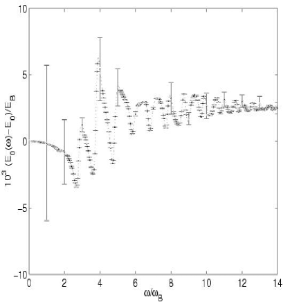
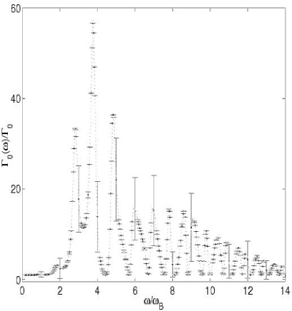
Figure 5.2: The real (left panel) and the imaginary (right panel) parts of the ground quasienergy resonances as function of the driving frequency $\omega$. The dashed line interpolates the average values $\bar{E}_{0}(\omega)$ and $\bar{\Gamma}_{0}(\omega)$ obtained for the rational values $\omega/\omega_{B}=p/q$ with $q\leq 7$ and $p\leq 98$. The “error bars” mark the bandwidths $\Delta^{\rm Re}_{0}(\omega)$ and $\Delta^{\rm Im}_{0}(\omega)$. The system parameters are $\hbar=2$, $F=0.061$ and $\varepsilon=0.08$.

We begin with the analysis of the real part of the spectrum, $E={\rm Re}\,\mathcal{E}$. Recalling the results of Sec. 5.1 the real part of the quasienergy spectrum is expected to obey

$$E_{\alpha}^{(n)}(\kappa)=\bar{E}_{\alpha}+\frac{2\pi Fn}{q}+\frac{\Delta_{\alpha}^{\rm Re}}{2}\,\cos(2\pi p\kappa)\;,\quad n=0,\ldots,p-1\;.$$ (5.35)

The left panel in Fig. 5.2 shows the mean position of the ground quasienergy bands (dots) and the band widths (marked as error bars) calculated for some rational values of the driving frequency $\omega$ (only the bands with $n=0$ are shown). The parameters of the non-driven system with $V(x)=\cos x$ are $\hbar=2$ and $F=0.061$. For these parameters the widths of two first resonances are $\Gamma_{0}=1.24\cdot 10^{-4}$ and $\Gamma_{1}=1.30\cdot 10^{-1}$. The distance between the real parts of the resonances is $E_{1}-E_{0}=3.784\hbar\omega_{B}$. It is seen in the figure that the band widths $\Delta_{0}^{\rm Re}=\Delta_{0}^{\rm Re}(\omega)$ are large only for $\omega=p\omega_{B}$, in qualitative agreement with the estimate (5.11). We would like to stress, however, that estimate (5.11) is obtained within the single-band approximation and, because of this, the actual bandwidths deviate from this dependence. (We shall discuss the conditions of validity of Eq. (5.11) later on in Sec. 5.4.) The second deviation from the predictions of single-band model is the dependence of the mean quasienergy band position $\bar{E}_{0}$ on $\omega$. As shown below, this dependence reflects the presence of the other quasienergy states, originating from the higher ($\alpha>0$) Bloch bands. Let us also note that the mean position $\bar{E}_{\alpha}=\bar{E}_{\alpha}(\omega)$ is, unlike the band width $\Delta_{\alpha}^{\rm Re}=\Delta_{\alpha}^{\rm Re}(\omega)$, a continuous function of the frequency.

The right panel in Fig. 5.2 shows the imaginary part $\Gamma=-2{\rm Im}\,\mathcal{E}$ of the quasienergy spectrum. In the perturbation regime $\varepsilon\rightarrow 0$ a behavior similar to (5.35),

$$\Gamma_{\alpha}(\kappa)\approx\bar{\Gamma}_{\alpha}+\frac{\Delta_{\alpha}^{\rm Im}}{2}\,\cos(2\pi\kappa)\;,$$ (5.36)

is observed. It should be noted that the smooth function $\bar{\Gamma}_{0}=\bar{\Gamma}_{0}(\omega)$ approximating the mean values of the bands is nothing else as the induced decay rate discussed in Sec. 4.1. In fact, an arbitrary initial state of the system (which was assumed to be the ground Wannier-Stark state $\Psi_{0,l}(x)$ in Sec. 4.1) can be expanded in the basis of the quasienergy states $\Psi_{\alpha}^{(n)}(x)$ as

$$\Psi(t=0)=\sum_{\alpha,n}c_{\alpha,n}\Psi_{\alpha}^{(n)}\;,\quad c_{\alpha}(n)=\langle\Psi_{\alpha}^{(n)}|\Psi(t=0)\rangle\;.$$ (5.37)

(Here we assume that $\omega/\omega_{B}$ is an irrational number and, therefore, the quasienergy functions are localized function with discrete spectrum.) During the time evolution the coefficients $c_{\alpha,n}(t)$ decay as $\exp(-\Gamma_{\alpha}t/2\hbar)$. Since $\Gamma_{\alpha}>\Gamma_{0}$ ($\alpha>0$), the projection of the wave function back to the initial state decays (after a short transient) exponentially with an increment given by $\bar{\Gamma}_{0}(\omega)/2$. This is the underlying argument of our numerical method of calculating the decay spectrum of the system. Namely, to obtain the decay spectrum discussed in chapter 4 we calculated the mean imaginary values of the quasienergy bands for a number of rational $\omega/\omega_{B}$ and then interpolate them for an arbitrary $\omega$.

Let us now discuss the $\omega$-dependence of the smooth functions $\bar{E}_{0}(\omega)$, $\bar{\Gamma}_{0}(\omega)$. Because we analyze the case of weak driving, these functions can be obtained by using perturbation theory. In fact, assuming again an irrational value of $\omega/\omega_{B}$, the zero order approximation of the most stable quasienergy function is the ground Wannier-Stark state $\Psi_{0,n}(x)$. According to the common perturbation theory, the first order correction is

$$\Psi_{0}^{(n)}=\Psi_{0,n}+F_{\omega}\sum_{\alpha,l}\sum_{\pm}\frac{\langle\Psi_{0,n}|x|\Psi_{\alpha,l}\rangle}{\mathcal{E}_{\alpha,l}-\mathcal{E}_{0,n}\pm\hbar\omega}\,\Psi_{\alpha,l}\;.$$ (5.38)

Correspondingly, the second oder correction to the energy is

$$\mathcal{E}_{0}^{(n)}=\mathcal{E}_{0,n}+\frac{F^{2}_{\omega}}{2}\sum_{\alpha,l}\sum_{\pm}\frac{V^{2}_{0,\alpha}(l-n)}{\mathcal{E}_{\alpha}-\mathcal{E}_{0}+(l-n)\hbar\omega_{B}\pm\hbar\omega}\;.$$ (5.39)

In Eq. (5.39) we used the notation (4.3) for the squared dipole matrix elements and took into account that the energies of the Wannier-Stark states form the ladder $\mathcal{E}_{\alpha,l}=\mathcal{E}_{\alpha}+l\hbar\omega_{B}$. Equation (5.39) is illustrated in Fig. 5.3, where the real (left panel) and imaginary (right panel) parts of the quasienergy calculated on the basis of this equation (solid line) are compared to the numerical data of Fig. 5.2 (dots, interpolated by a dashed line). For small (relative to $\omega_{B}$) frequencies both curves coincide almost perfectly, but deviate for large $\omega$. This deviation can be attributed to the slow convergence of the perturbation series over $\alpha$ in the high-frequency region. (For the presented results, the upper limit for the sum over the Wannier-Stark ladders is taken as $\alpha=3$.)

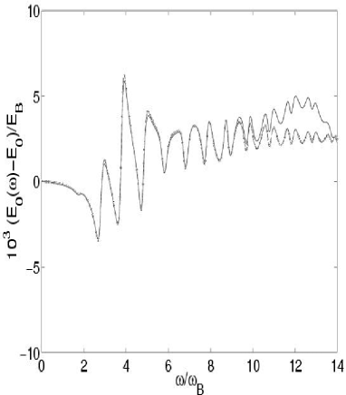
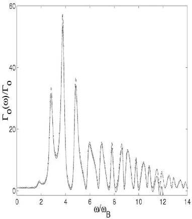
Figure 5.3: Corrections to the ground state energy from Fig. 5.2 (dashed line) compared to approximations based on equation (5.39) (solid line). The left panel shows the real part of the ground state energy, the right panel the imaginary part.

The concluding remark of this section concerns the relation between Eq. (4.2) [i.e. the imaginary part of Eq. (5.39)] and the “$\varepsilon$-version” of Eq. (4.2) used to analyze the decay spectrum of atoms in optical lattices in Sec. 4.3. The difference is the use of the squared matrix elements (4.17) instead of the squared dipole matrix elements (4.3). However, recalling the relation $\varepsilon=F_{\omega}/\omega^{2}$ and relation (4.19), this difference can be shown to be within the accuracy of the second order perturbation theory. The advantage of the $\varepsilon$-version over the $F_{\omega}$-version is a better convergence in the high-frequency region.

5.4 Perturbation theory for rational frequencies

Discussing the perturbation approach in the previous section we excluded the case of rational ratio of the driving and Bloch frequencies. Let us now turn to it. To be concrete, we restrict ourselves by the simplest but important case $\omega=\omega_{B}$. In this case the periodic driving couples the Wannier-Stark states belonging to the same Wannier-Stark ladder and, therefore, the extended Wannier-Bloch function $\Phi_{\alpha,\kappa}$ is an appropriate zero order approximation to the quasienergy function.

As described in the beginning of this chapter, the complex quasienergies of the system are found by solving the eigenvalue equation

$$U(T_{\omega})\Phi_{\alpha,\kappa}=\exp[-{\rm i}\mathcal{E}_{\alpha}(\kappa)T_{\omega}/\hbar]\,\Phi_{\alpha,\kappa}\;.$$ (5.40)

Let us approximate the Hamiltonian (5.2) by the first order of the Taylor expansion in $\varepsilon$, $H\approx H_{W}-\varepsilon\sin(x)\cos(\omega t)$ (here $H_{W}$ is the Wannier-Stark Hamiltonian (2.2) and $V(x)=\cos x$ is assumed for simplicity). Then we can calculate the effect of the periodic driving in the interaction representation of the Schrödinger equation. Explicitly, we get

$$U(T_{\omega})\approx U_{\varepsilon}(T_{\omega})\,U_{W}(T_{\omega})$$ (5.41)

where the operator $U_{\varepsilon}(T_{\omega})$ reads

$$U_{\varepsilon}(T_{\omega})=\widehat{\exp}\left(\frac{{\rm i}\varepsilon}{\hbar}\int_{0}^{T_{\omega}}{\rm d}t\,\cos(\omega t)\,U^{\dagger}_{W}(t)\,\sin(x)\,U_{W}(t)\right)\;,$$ (5.42)

and the operator $U_{W}(t)$ is the evolution operator for the unperturbed system. According to common perturbation theory, the first order correction is given by the diagonal elements of the operator $U_{\varepsilon}(T_{\omega})$,

$$\exp[-{\rm i}\Delta\mathcal{E}_{\alpha}(\kappa)T_{\omega}/\hbar]=\langle\Phi_{\alpha,\kappa}|\,U_{\varepsilon}(T_{\omega})\,|\Phi_{\alpha,\kappa}\rangle\,.$$ (5.43)

Let us approximate this formula further. Expanding the operator exponent in a series in $\varepsilon$ and keeping only the first term, the correction to the quasienergy reads

$$\Delta E_{\alpha}(\kappa)=-\frac{\varepsilon}{T_{\omega}}\int_{0}^{T_{\omega}}{\rm d}t\,\cos(\omega t)\,\langle\Phi_{\alpha,\kappa}|\,U^{\dagger}_{W}(t)\,\sin(x)\,U_{W}(t)\,|\Phi_{\alpha,\kappa}\rangle\;.$$ (5.44)

Using the solution $U_{W}(t)\Phi_{\alpha,\kappa}=\exp(-{\rm i}\mathcal{E}_{\alpha}t/\hbar)\,\Phi_{\alpha,\kappa-Ft/\hbar}$ and substituting ${\rm d}t/T_{\omega}=-{\rm d}\kappa$,
Eq. (5.44) takes the form

$$\Delta\mathcal{E}_{\alpha}(\kappa)=-\varepsilon\int_{0}^{1}{\rm d}\kappa^{\prime}\cos(2\pi\kappa^{\prime})\,\langle\Phi_{\alpha,\kappa+\kappa^{\prime}}|\sin(x)|\Phi_{\alpha,\kappa+\kappa^{\prime}}\rangle\;.$$ (5.45)

Finally, using the symmetry property of the Wannier-Bloch function, the integral (5.45) can be presented in the form

$$\Delta\mathcal{E}_{\alpha}(\kappa)=\left(\frac{\Delta^{\rm Re}_{\alpha}+{\rm i}\Delta^{\rm Im}_{\alpha}}{2}\right)\cos(2\pi\kappa)\;,$$ (5.46)

where

$$\Delta^{\rm Re}_{\alpha}+{\rm i}\Delta^{\rm Im}_{\alpha}=-2\varepsilon\int_{0}^{1}{\rm d}\kappa\,\cos(2\pi\kappa)\,\langle\Phi_{\alpha,\kappa}|\sin(x)|\Phi_{\alpha,\kappa}\rangle\,.$$ (5.47)

(The special notation for the band width stresses that the integral on the right hand side of Eq. (5.47) is a complex number.) Thus, a weak periodic driving removes the degeneracy of the Wannier-Bloch bands which then gain a finite width. Moreover, there are corrections both to the real and imaginary part of the quasienergy.

In conclusion, let us briefly discuss the relation between the formulas (5.46), (5.47) and the tight-binding result (5.12). As was stated many times, the single-band model neglects the interband tunneling, which is justified in the limit $F\rightarrow 0$. In this limit the quasienergy band width can be estimated as

$$\Delta^{\rm Re}_{\alpha}=\varepsilon\frac{4\pi^{2}F\Delta_{\alpha}}{\hbar^{2}}=\Delta_{\alpha}\frac{F_{\omega}}{F}\;,$$ (5.48)

where $\Delta_{\alpha}$ is the width of the Bloch band. Indeed, using Eq. (4.18), the band width in Eq. (5.47) can be expressed in terms of the dipole matrix elements as

$$\Delta^{\rm Re}_{\alpha}+{\rm i}\Delta^{\rm Im}_{\alpha}=\varepsilon\frac{(2\pi F)^{2}}{\hbar^{2}}\,\Big{(}\,\langle\Psi_{\alpha,1}|x|\Psi_{\alpha,0}\rangle+\langle\Psi_{\alpha,0}|x|\Psi_{\alpha,1}\rangle\,\Big{)}\;.$$ (5.49)

Then, using the tight-binding approximation (1.11) for the resonance Wannier-Stark states $\Psi_{\alpha,1}(x)$, we obtain the estimate (5.48). (Alternatively, we can approximate $\chi_{\alpha,\kappa}(x)$ in Eq. (4.14) by the periodic part of the Bloch function.) It is seen, that the estimate (5.48) coincides with Eq. (5.12) in the limit $F_{\omega}/F\rightarrow 0$. We would like to stress, however, that the actual perturbation parameter of the problem is $\varepsilon\sim F_{\omega}/F^{2}$ and not $F_{\omega}/F$, as it could be naively expected on the basis of the tight-binding model.

5.5 Selective decay

This section serves as an illustration to the perturbation theory of Sec. 5.4 and discusses some important limitations of the perturbation approach. In order to reduce the number of relevant resonance states, we choose the parameters of the unperturbed system as $\hbar=2$, $F=0.08$. In this case we have to take into account mainly two resonances with energies $\mathcal{E}_{0}=9.42\cdot 10^{-2}-{\rm i}5.60\cdot 10^{-4}$ and $\mathcal{E}_{1}=4.18\cdot 10^{-2}-{\rm i}8.81\cdot 10^{-2}$. All other resonances are very unstable and approximately do not influence the results. The frequency of the time-periodic perturbation is given by $\omega=2\pi F/\hbar\approx 0.251$.

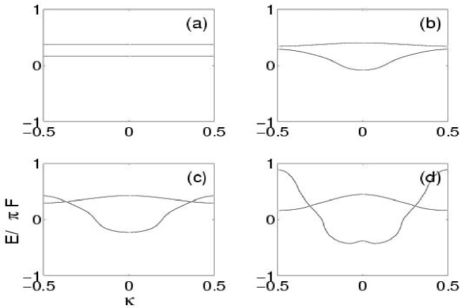
Figure 5.4: Real part of the two most stable (quasi-)energy Wannier-Bloch bands for $\varepsilon=0$ (a), $\varepsilon=0.2$ (b), $\varepsilon=0.4$ (c) and $\varepsilon=1$ (d). The other system parameters are $\hbar=2$, $F=0.08$ and $\omega=2\pi F/\hbar\approx 0.251$.

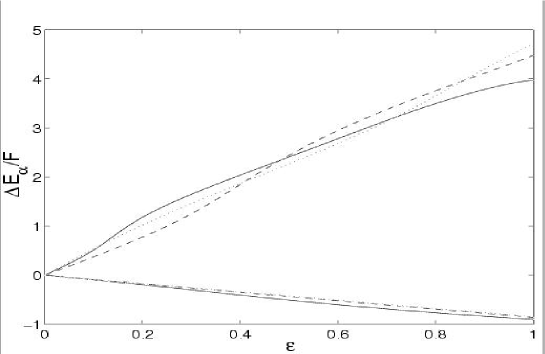
Figure 5.5: Band width of the two most stable Wannier-Bloch bands as a function of the perturbation parameter $\varepsilon$ for $F=0.08$ (solid line), $F=0.04$ (dashed line) and $F=0.02$ (dotted line).

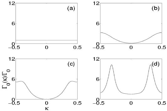
Figure 5.6: Width (decay rate) of the ground state as a function of the Bloch index $\kappa$ for the cases studied in Fig. 5.4. The width is normalized with respect to the width at $\varepsilon=0$.

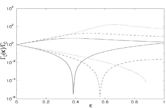
Figure 5.7: Decay rate of the most stable Wannier-Bloch state at $\kappa=0$ (lower family of curves) and $\kappa=\pm 1/2$ (upper family of curves) for the same parameters as in Fig. 5.5, i.e. $F=0.08$ (solid line), $F=0.04$ (dashed line) and $F=0.02$ (dotted line). The rate is normalized against the decay rate at $\varepsilon=0$.

Figure 5.4 shows the real parts of the quasienergies of the two most stable Wannier-Bloch resonances for different amplitudes $\varepsilon$. In panel (a) we have the unperturbed case with flat bands. When the ac driving is added, the dispersion relation of the ground band is well described by the theoretical cosine dependence. The first excited band follows this relation only up to $\varepsilon=0.2$. If the amplitude is increased further, deviations from the cosine appear, and for $\varepsilon=1$ other effects strongly influence the band (note that in this case $F_{\omega}/F\approx 0.79$, thus we are still far away from the parameter range where the tight-binding model predicts dynamical band suppression). Furthermore, for $\varepsilon>0.2$ the bands cross, and then we cannot neglect their interaction.

Next we investigate the bandwidth, i.e. the difference between the extrema of the real parts of the quasienergies, $\Delta E\!=\!E(\kappa\!=\!1/2)-E(\kappa\!=\!0)$. Figure 5.5 shows the width of the two most stable bands as a function of the amplitude $\varepsilon$ for three different field strengths $F=0.02$, $F=0.04$ and $F=0.08$. It is seen that in all cases the bandwidth grows approximately linearly. Again, the agreement is much better for the ground band; for the first excited band one observes an oscillation around the linear growth. Note that the slope is proportional to $F$ as expected on the basis of the perturbation theory [see Eq. (5.48)].

We proceed with the analysis of the imaginary part of the quasienergy spectrum. Figure 5.6 shows the width of the ground state as a function of the Bloch index for the parameters of Fig. 5.4. For $\varepsilon=0$ the band is flat as predicted from the theory. For $\varepsilon=0.2$ the width can be approximated by a cosine, however, the mean is shifted to approximately twice the unperturbed width. If we further increase $\varepsilon$, additional structures appear. In comparison with Fig. 5.4, we see that the bandwidth is increased where the (real part of the quasienergy of the) ground band crosses the first excited band. Therefore, we can clearly assign the increase of the width to the band crossings. Recalling the results of chapter 3, we again observe effects of resonant tunneling, now as a function of the quasimomentum. As shown in Ref. [156, 164], the two-state model of Sec. 3.3 can be adopted to the present case and yields good correspondence to the numerical data.

In Fig. 5.6 we can see that the perturbation can both increase and decrease the width and thus the rate of decay of the quasienergy states. In the case considered, for small $\varepsilon$ the decay is enhanced at the edges of the Brillouin zone and suppressed in its center. Let us therefore take these two quasimomenta to further investigate the dependence on the perturbation parameter $\varepsilon$. The results of a calculation of the widths at $\kappa=0$ and $\kappa=\pm 1/2$ as a function of the amplitude $\varepsilon$ are shown in figure 5.7. For small $\varepsilon$ the dependence is nearly linear, but for larger values it is highly nontrivial. In particular, we would like to draw the attention to the behavior of the solid line at $\varepsilon\approx 0.4$ and of the dashed line at $\varepsilon\approx 0.54$. Here the decay rate is suppressed by more than a factor $10^{5}$! This tremendous decrease of the decay rate has enormous consequences on the global dynamics. For example, let us initially take the most stable Wannier-Stark state and then add the ac driving. Then the survival probability is given by

$$P(t)=\int_{-1/2}^{1/2}{\rm d}\kappa\exp\left(-\frac{\Gamma_{0}(\kappa)\,t}{\hbar}\right)\;.$$ (5.50)

If we approach the critical value $\varepsilon_{\rm cr}$, the decay is suppressed and asymptotically

$$P(t)\sim t^{-1/2}\exp(-\Gamma_{\rm min}\,t/\hbar)\;,$$ (5.51)

where $\Gamma_{\rm min}$ is the minimal decay rate. Let us also note another property. Since the decay rate of the quasienergy states depend on the quasimomentum, after some time only the contributions with quasimomentum around the value with the smallest decay rate will survive. In what follows we shall refer to this phenomenon as the selective decay of the quasienergy states. Some physical consequence of this phenomenon are discussed in the next chapter.

Chapter 6 Wave packet dynamics

In this section we address the question of the time evolution of an initially localized wave packet. Usually this problem is analyzed by simulating the wave packet dynamics on the basis of the time-dependent Schrödinger equation. However, this numerical approach is very time consuming and has an upper limit for the times considered. In what follows we describe the evolution of the wave packet in terms of the resonance states. Besides tremendous decrease of the computational efforts, the latter approach also gives additional insight into the decay process of the Wannier-Stark states.

6.1 Expansion over resonance states

A direct expansion of a localized state in terms of resonances yields inappropriate results because in the negative $x$-direction the resonance states extend to infinity. Therefore the description needs to be modified to take into account the finite extension of the initial state. Recently this problem was analyzed for decaying quantum systems with a finite range potential [183, 184].

Let us adopt the approach of [184] to describe the evolution of the wave packet in momentum space. In this approach, the wave function $\psi(k,t)$ is expressed in terms of the stationary scattering states $\Psi_{S}(k;E)$:

$$\psi(k,t)=\int_{-\infty}^{\infty}{\rm d}E\,f(E)\,\Psi_{S}(k;E)\,\exp\left(-{\rm i}\,\frac{Et}{\hbar}\right)\;,$$ (6.1)

where $f(E)=\langle\Psi_{S}(k;E)|\psi(k,0)\rangle$. [We recall that the states $\Psi_{S}(k;E)$ are normalized to $\delta$-function: $\langle\Psi_{S}(k;E^{\prime})|\Psi_{S}(k;E)\rangle=\delta(E-E^{\prime})$.] We are mainly interested in the properties of the decay tail at $k\rightarrow-\infty$. In this region the scattering states can be approximated by their asymptotic form [see Eq. (2.7)]

$$\lim_{k\rightarrow\pm\infty}\Psi_{\pm}(k;E)=g_{\pm}(E)\,\exp\left({\rm i}\,\frac{\hbar^{2}k^{3}}{6F}-{\rm i}\,\frac{Ek}{F}\right)\;,\quad g_{\pm}(E)=e^{\pm{\rm i}\varphi(E)}\;.$$ (6.2)

Substituting this asymptotic form into Eq. (6.1) we have

$$\psi(k,t)=\exp\left({\rm i}\,\frac{\hbar^{2}k^{3}}{6F}\right)\,G_{-}\left(k+\frac{Ft}{\hbar}\right)\,,\quad k\ll 0\;,$$ (6.3)

where

$$G_{-}(k)=\int_{-\infty}^{\infty}{\rm d}E\,\frac{f(E)}{g_{+}(E)}\,\exp\left(-{\rm i}\,\frac{Ek}{F}\right)\;.$$ (6.4)

If the initial wave function $\psi(k,0)$ has a finite support, $f(E)$ is an entire function in the complex plane. Then the function $f(E)/g_{+}(E)$ has simple poles at zeros of $g_{+}(E)$, i.e at the poles of the scattering matrix $S(E)=g_{-}(E)/g_{+}(E)$. This property suggests to evaluate the integral (6.4) with the help of the residuum theorem. Without knowing the explicit form of the function $f(E)/g_{+}(E)$ we have to make some assumptions on its asymptotic behavior in order to proceed further. In particular, if we assume that the function $f(E)/g_{+}(E)$ does not influence the behavior of the integrand at infinity, the integral yields a sum over the residua located within the appropriate contour. Explicitly, for $k>0$ the contour should be closed in the lower half of the complex plane, for $k<0$ it contains the upper half. Since all poles of the scattering matrix are located in the lower half of the complex plane, we get

$$G_{-}(k)=2\pi{\rm i}\,\Theta\left(k\right)\sum_{\nu}b_{\nu}\exp\left(-{\rm i}\,\frac{\mathcal{E}_{\nu}k}{F}\right)\,,$$ (6.5)

where $\Theta(k)$ is the Heaviside function, the $b_{\nu}$ are the residua of $f(E)/g_{+}(E)$ at the poles, and $\nu=\{\alpha,l\}$. Inserting this result in (6.3) yields

$$\psi(k,t)=\Theta\left(\hbar k+Ft\right)\sum_{\nu}c_{\nu}\exp\left[{\rm i}\left(\frac{\hbar^{2}k^{3}}{6F}-\frac{\mathcal{E}_{\nu}k}{F}-\frac{\mathcal{E}_{\nu}t}{\hbar}\right)\right]\;,$$ (6.6)

with $c_{\nu}=2\pi{\rm i}b_{\nu}$. The terms of the sum are actually proportional to the asymptotic form of the resonance wave functions $\Psi_{\nu}(k,t)$. Thus, we can equivalently present the wave function as

$$\psi(k,t)=\Theta\left(\hbar k+Ft\right)\sum_{\nu}c_{\nu}\,\exp\left(-{\rm i}\,\frac{\mathcal{E}_{\nu}t}{\hbar}\right)\Psi_{\nu}(k)\;.$$ (6.7)

Therefore, in the Stark case we can describe the evolution of an initial state by a superposition of resonances, where we take into account the space-time decay process in the prefactor $\Theta\left(\hbar k+Ft\right)$. This factor truncates the wave function at the momentum $\hbar k=-Ft$, i.e. only momenta with $\hbar k>-Ft$ contribute. With increasing time, the wave function extends to smaller momenta, where the edge moves according to the classical equation of motion.

It should be noted that the location of the edge reflects the assumption on the behavior at infinity we made in order to explicitly evaluate the integral. For example, the function $f(E)/g_{+}(E)$ may contain an additional exponential factor $\exp({\rm i}\alpha E)$ (see the example in [184]). Though this factor does not influence the poles, it nevertheless influences the argument of the Heaviside function. In fact, in a realistic situation the edge will be shifted, because the truncation edge at $t=0$ has to reflect the extension of the initial state in momentum space. We take this into account by replacing $\hbar k$ in the argument of the Heaviside function by $\hbar(k+k_{0})$, where $k_{0}$ describes the extension of the initial state in the negative $k$-direction. Furthermore, if the initial state does not have a compact support but a tail in the negative momentum direction, the edge will be smoothed and deformed. However, the qualitative behavior remains unchanged: the prefactor is approximately constant for positive arguments of the Heaviside function, and it approximately vanishes for negative arguments. Therefore, we take the Heaviside description as a reasonable approximation to the real situation. Let us also note that the wave function constructed in this way can be normalized. Indeed, in the positive momentum direction the resonances decrease stronger than exponentially, and in the negative direction the wave function is truncated.

Now we discuss the dynamics of the wave packet in coordinate space. If we are interested in the asymptotic behavior for $x\ll 0$, the wave function $\psi(x,t)$ can be found by a Fourier transform of the asymptotic form of Eq. (6.7):

$$\psi(x,t)=\int_{-\infty}^{\infty}\!\!{\rm d}k\,\Theta[\hbar(k+k_{0})+Ft]\sum_{\nu}c_{\nu}\exp\left[{\rm i}\left(\frac{\hbar^{2}k^{3}}{6F}-\frac{\mathcal{E}_{\nu}k}{F}-\frac{\mathcal{E}_{\nu}t}{\hbar}+kx\right)\right]\;.$$ (6.8)

Let us evaluate the integral in the stationary phase approximation. The equation for the stationary phases reads

$$\frac{{\rm d}}{{\rm d}k}\left(\frac{\hbar^{2}k^{3}}{6F}-\frac{k\mathcal{E}_{\nu}}{F}+kx\right)=0\;.$$ (6.9)

Neglecting the imaginary part of the energy $\mathcal{E}_{\nu}$ , the stationary phase condition is just the energy conservation, and the stationary points are the classical momenta $\hbar k_{\nu}=\sqrt{2(E_{\nu}-Fx)}=p_{\nu}(x)$. If $p_{\nu}(x)\ll-\hbar k_{0}-Ft$, the prefactor is zero and the integral vanishes. On the other hand, if $p_{\nu}(x)\gg-\hbar k_{0}-Ft$, the integral of the contribution of the $\nu$-th resonance yields approximately

$$\exp\left(-{\rm i}\frac{\mathcal{E}_{\nu}t}{\hbar}\right)\,\sqrt{\frac{2\pi F}{\hbar p_{\nu}(x)}\,}\,\exp\left(-{\rm i}\frac{p_{\nu}^{3}(x)}{3\hbar F}-\frac{\Gamma_{\nu}p_{\nu}(x)}{2\hbar F}\right)\;,$$ (6.10)

which is just the asymptotic form of the Wannier-Stark state in the coordinate representation. The critical point is $p_{\nu}(x)=-\hbar k_{0}-Ft$, where the approximation breaks down because the Heaviside function is not a slowly varying function at this point. Actually, in the vicinity of this point the integral interpolates between the other two possibilities. Let us skip a more detailed analysis here and roughly describe the transition between both regimes by a Heaviside function of the argument $p_{\nu}(x)+\hbar k_{0}+Ft$, or, equivalently, of the argument $x+F(t+t_{0})^{2}/2-E_{\nu}/F$, where $t_{0}=\hbar k_{0}/F$. Then, replacing the contribution (6.10) by $\Psi_{\nu}(x,t)$, we get

$$\psi(x,t)=\sum_{\nu}\,c_{\nu}\,\Theta\left[x+\frac{F(t+t_{0})^{2}}{2}-\frac{E_{\nu}}{F}\right]\,\exp\left(-{\rm i}\,\frac{\mathcal{E}_{\nu}t}{\hbar}\right)\Psi_{\nu}(x)\,.$$ (6.11)

In comparison to equation (6.7) there are two differences. First, in coordinate space the truncation depends on the energy of the resonances. Furthermore, the edges of the different contributions move with a quadratic time dependence, which reflects the classical (accelerated) motion in a constant external field.

6.2 Pulse output from Wannier-Stark systems

Let us consider the dynamics of a coherent superposition of the Wannier-Stark resonances belonging to a particular Wannier-Stark ladder

$$\psi(k,t)=\sum_{l}c_{l}\exp\left(-{\rm i}\,\frac{\mathcal{E}_{\alpha,l}t}{\hbar}\right)\,\Psi_{\alpha,l}(k)\;,\quad c_{l}=\frac{1}{\sqrt{\pi}\sigma}\exp\left(-\frac{l^{2}}{\sigma^{2}}\right)\;.$$ (6.12)

(To shorten the notation, we skip here the truncation by the Heaviside function because the truncation does not influence the properties which we are going to discuss). This problem, as will be seen later on, is directly related to the experiment [126], where a coherent pulse output of cold atoms was observed. Based on this phenomenon, a possibility of constructing an atomic laser is currently discussed in the literature.

According to Eq. (2.39) the Wannier-Stark states belonging to the same ladder are related by $\Psi_{\alpha,l}(k)=\exp(-{\rm i}2\pi lk)\,\Psi_{\alpha,0}(k)$ and $\mathcal{E}_{\alpha,l}=\mathcal{E}_{\alpha}+2\pi lF$. Combining this phase relation with the different phases due to the time evolution, the time evolution of the superposition is given by

$$\psi(k,t)=\Psi_{\alpha,0}(k,t)\,\widetilde{C}\left(\frac{Ft}{\hbar}+k\right)\;,\quad\widetilde{C}(k)=\sum_{l}c_{l}\,\exp(-{\rm i}2\pi lk)\;.$$ (6.13)

where $\Psi_{\alpha,0}(k,t)=\exp(-{\rm i}\mathcal{E}_{\alpha}t/\hbar)\Psi_{\alpha,0}(k)$. Thus, the time evolution of the superposition is given by the time-evolved wave function at the mean energy, $\Psi_{\alpha,0}(k,t)$, times the discrete Fourier transform $\widetilde{C}(k)$ of the amplitudes $c_{l}$, which is taken at the momenta $k+Ft/\hbar$. Since the function $\widetilde{C}(k)$ is periodic in momentum space the factor $\widetilde{C}(k+Ft/\hbar)$ is also periodic in time with the period $\hbar/F=T_{B}$. In what follows we shall refer to the function $\widetilde{C}(k)$ as amplitude modulation factor. In the considered case $c_{l}\sim\exp(-l^{2}/\sigma^{2})$ the amplitude modulation factor is obviously a periodic train of Gaussians with the width $\sigma^{-1}$.

We turn to the coordinate representation. Following the derivation of the preceding section, the wave function $\psi(x,t)$ can be shown to obey

$$\psi(x,t)=\Psi_{\alpha,0}(x,t)\,\widetilde{C}\left(\frac{t}{T_{B}}+\frac{p(x)}{\hbar}\right)\;,$$ (6.14)

where, as before, $p(x)=\sqrt{2(E_{\alpha}-Fx)}$ is the classical momentum. Because the function $\widetilde{C}(k)$ has peaks at integer values of the arguments, the function $\widetilde{C}(t/T_{B}+p(x)/\hbar)$ has peaks at the coordinates

$$x=x_{0}-\frac{F}{2}\,(t+mT_{B})^{2}\,,$$ (6.15)

where $x_{0}=E_{\alpha}/F$ is the classical turning point. Thus, as a function of time, the peaks accelerate according to the classical equation of motion of a free particle subject to a constant electric field. Additionally, the peaks broaden linearly with increasing time (or with increasing $m$). It is straightforward to combine the result (6.14) with the result of the previous sections. Generally, we have to truncate the wave front approximately at the coordinate $x=-F(t+t_{0})^{2}/2$.

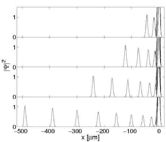
Figure 6.1: Space-time decay of the wave packet for the parameters of the experiment [126]. From top to bottom, the panels correspond to $t=3\,{\rm ms}$, $5\,{\rm ms}$, $7\,{\rm ms}$ and $10\,{\rm ms}$, respectively.

Figure 6.1 shows the evolution of the superposition of the ground Wannier-Stark resonances for $V(x)=\cos x$. The system parameters are $\hbar=3.3806$, $F=0.0661$ and $\sigma=15$, which correspond to the setting of the experiment [126]. The figure was calculated in the following way: First the ground $l=0$ Wannier-Stark state was calculated in the momentum representation. Then the wave function was multiplied with the amplitude modulation factor $\widetilde{C}(Ft/\hbar+k)$ taken at the specified times and truncated according to equation (6.7). (We shifted the truncation edge by $k_{0}=1/2$ in order to avoid a truncation directly at the maxima. As mentioned in Sec. 6.1 this shift takes into account the finite extension of the initial state.) Finally the resulting function was Fourier transformed into coordinate space. The obtained result reproduces the findings of the experiment [126]. A series of pulses is formed which then accelerate according to the free motion. At a fixed value of the coordinate, the sequence is periodic in time (after the first pulse passed), up to an overall exponential decay which reflects the fact that every pulse takes away a certain amount of probability.

A few words should be added about the validity of the one-particle approximation. In fact, in the experiment cited, the authors used a Bose-Einstein condensate of Rubidium atoms, uploaded in a vertically aligned optical lattice. Thus a description of the system with the help of the Gross-Pitaevskii equation

$${\rm i}\hbar\partial_{t}\Psi=\left[\frac{p^{2}}{2M}+V_{0}\cos(2k_{L}z)+Mgz+V_{\rm int}|\Psi|^{2}\right]\Psi\,,$$ (6.16)

looks more appropriate. Equation (6.16) was studied numerically in Ref. [187, 188, 189, 190, 191, 192, 193]. It was found that for moderate densities of the condensate (realized in practice) the pulse formation is only slightly modified by the nonlinear term in the Gross-Pitaevskii equation. Thus the physics behind the experimentally observed phenomenon is provided by single-particle quantum mechanics and can be well understood in terms of Wannier-Stark resonance states.

6.3 Atom laser mode-locking

The crucial point for the existence of the pulse output in the Wannier-Stark system is the fixed phase relation between the probability amplitude $c_{l}$ in Eq. (6.12). In the experiment [126], this fixed phase relation was achieved by the self-interaction of the Bose condensate. In the following we show that one can prepare an appropriate initial state within single particle quantum mechanics. Explicitly, the statement is as follows. Take an arbitrary initial state (i.e. arbitrary $c_{l}$) and drive the system for a finite time $T_{\rm int}$ with the frequency matching the Bloch frequency $\omega_{B}$. If the driving amplitude is sufficiently large and the interaction time $T_{\rm int}$ is long enough, the initial state decays with a pulse output afterwards.

The physics behind this effect is the selective decay of the quasienergy Wannier-Bloch state discussed in Sec. 5.5. Indeed, let the $\Phi_{\alpha,\kappa}(k)$ be the quasienergy states of the dc-ac Hamiltonian (5.2). Then we can expand the initial state $\psi(k,0)$ in this basis

$$\psi(k,0)=\sum_{\alpha}\int_{-1/2}^{1/2}{\rm d}\kappa\,c_{\alpha}(\kappa)\,\Phi_{\alpha,\kappa}(k)\,,$$ (6.17)

where the $c_{\alpha}(\kappa)$ are periodic functions of the quasimomentum. [In particular, assuming the adiabatic switching of the field, the initial condition $\psi(k,0)=\Psi_{0,l}(k)$ will correspond to $c_{\alpha}(\kappa)=\delta_{\alpha,0}\exp({\rm i}\kappa l)$.] Note that the expansion (6.17) is also valid in the case of a pure dc field considered in the previous section, but we preferred there the alternative basis of the Wannier-Stark states [see Eq. (6.12)]. After $N$ periods of driving the wave function reads

$$\psi(k,NT_{B})\approx\int_{-1/2}^{1/2}{\rm d}\kappa\,c_{0}(\kappa)\,\exp\left(-{\rm i}\,\frac{\mathcal{E}_{0}(\kappa)NT_{B}}{\hbar}\right)\,\Phi_{0,\kappa}(k)\,,$$ (6.18)

where we assumed that all quasienergy states, excluding the ground states $\alpha=0$, have decayed. Now the ac field is switched off, and we take the final state $\psi(k,NT_{B})$ as the initial state of the pure dc dynamics. Expanding it in the basis of the Wannier-Stark states yields $\psi(k,NT_{B})=c_{0}(k)\,\exp(-{\rm i}\mathcal{E}_{0}(k)NT_{B}/\hbar)\,\Psi_{0,0}(k)$, where the functions $c_{0}(\kappa)$ and $\mathcal{E}_{0}(\kappa)$ are treated now as the periodic function of the momentum instead of the quasimomentum. Then

$$\psi(k,t>NT_{B})=\Psi_{\alpha,0}(k,t)\,\widetilde{C}\left(\frac{Ft}{\hbar}+k\right)\,,\quad\widetilde{C}(k)=c_{0}(k)\,\exp\left(-{\rm i}\,\frac{\mathcal{E}_{0}(k)NT_{B}}{\hbar}\right)\;.$$ (6.19)

Comparing this result with Eq. (6.13), we notice that the prefactor $c_{0}(k)\exp(-{\rm i}\mathcal{E}_{0}(k)NT_{B}/\hbar)$ takes the role of the amplitude modulation factor $\widetilde{C}(k)$ of the new initial state. Let us discuss this factor in more detail.

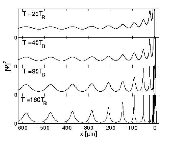
Figure 6.2: Tail of the wave function after the system was driven for different times $T=NT_{B}$. The parameters are $\hbar=3.3806$, $F=0.0661$ and $\varepsilon=0.1$.

As shown in Sec. 5.4, for small $\varepsilon$ the dispersion relation of the complex quasienergy band is $\mathcal{E}_{0}(\kappa)=\mathcal{E}_{0}+(\Delta_{0}^{\rm Re}/2+{\rm i}\Delta_{0}^{\rm Im}/2)\cos(2\pi\kappa)$. Thus the absolute value of the amplitude modulation factor is given by

$$|\widetilde{C}(k)|^{2}=|c(k)|^{2}\exp\left[-\frac{\Gamma_{0}NT_{B}}{\hbar}-\frac{\Delta_{0}^{\rm Im}NT_{B}}{2\hbar}\cos(2\pi k)\right]\,.$$ (6.20)

If the interaction time $T_{\rm int}=NT_{B}$ is large enough (and if $c(k)$ is sufficiently smooth), the strong modulation of the exponential dominates the form of the amplitude modulation factor. Then the wave function is periodically peaked in momentum space. Of course, such a periodically peaked structure is also found for larger values of $\varepsilon$ where formula (5.46) is no longer valid. In fact, due to the stronger modulation of $\Gamma_{0}(\kappa)$, it appears even for short interaction times.

The behavior of the wave function in coordinate space is additionally modified by the dispersion due to the real parts of the quasienergies. If we approximate it by the cosine and again apply the stationary phase approximation in the Fourier transform of equation (6.19), the stationary points $k_{s}$ are solutions of the slightly modified equation $\hbar^{2}k_{s}^{2}/2+\pi\Delta_{0}{\rm Re}N\sin(2\pi k_{s})=E_{0}-Fx$. The implications are as follows. In coordinate space, the form of the peaks is changed compared to the dispersion-free case, in particular, the peaks can be broadened or narrowed. Note that for small $|k_{s}|$ there may be three instead of one stationary point for each branch of the square root. Then the wave function shows additional interferences due to the interaction of the three different contributions. However, for large $|k_{s}|$ (i.e. for $x\rightarrow-\infty$), the dispersion only slightly influences the shape of the peaks. Thus, for large $|x|$, the shape of the peaks of the decay tail mainly reflects the function $\Gamma_{0}(\kappa)$, which provides a method to experimentally access of this function.

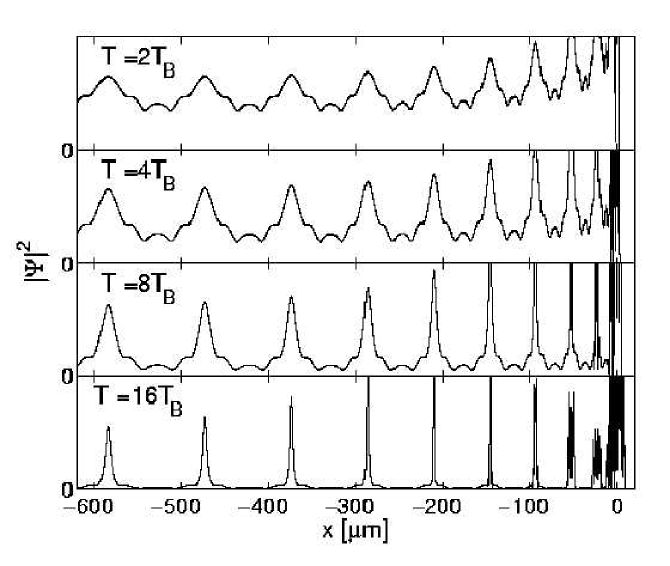
Figure 6.3: The same as in Fig. 6.2 but $\varepsilon=1.5$.

To support the above analysis, Fig. 6.2 shows the decay tails which develop for a weak driving with $\varepsilon=0.1$. In this numerical example we choose the ground Wannier-Stark resonance $\Psi_{0,0}(x)$ as the initial state (the other parameters are the same as in Fig. 6.1) and drive the system for different interaction time. (Explicitly, we calculated the resonances wave function $\Psi_{0,0}(k)$, multiplied by the amplitude modulation factor $\exp(-{\rm i}\mathcal{E}_{0}(k)NT_{B}/\hbar)$, where the dispersion relation was calculated independently, and finally Fourier transformed to coordinate space.) After short interaction times, the tail is slightly modulated. For longer interaction times, the modulation depth increases and pulses develop, which finally are clearly separated. Note that, apart from effects due to the dispersion, we can decrease the width of the pulses by further increasing the interaction time, which provides a simple way to tune the width experimentally.

A crucial point of the weak driving regime is the long interaction time which is needed to generate well separated pulses. The relevant timescale is set by the most long-lived state from the ground band. For the case $\varepsilon=0.1$, the minimum width is $\Gamma_{\rm min}=7.214\cdot 10^{-3}$, which corresponds to a lifetime approximately $10\,T_{B}$. Thus, the interaction time is much longer than the lifetime of the most stable state. Consequently, a predominant part of the initial wave packet has already decayed before pulses are being formed. One can, however, surmount this problem by increasing the amplitude of the resonant driving. Figure 6.3 shows the decay tail for $\varepsilon=1.5$. Now the pulses develop after much shorter interaction times. For $\varepsilon=1.5$, the function $\Gamma_{0}(\kappa)$ has four minima, which are due to two crossings with higher excited Wannier-Stark ladders (see Sec. 5.4). Note that one can directly read off this property from the substructure of the pulses on the decay tail. In the lower panels of the figure one can also see the narrowing caused by the dispersion. In particular, the first peaks (counted from the right) strongly oscillate, which reflects the existence of three stationary points in this region. However, the last peaks have approximately the same shape, i.e. here the narrowing effect can be neglected.

Chapter 7 Chaotic scattering

This chapter continues the analysis of Wannier-Stark system affected by an ac field. In chapters 5-6 we have considered the case of a relatively large scaled Planck constant $\hbar$ (see Sec. 1.4) and relatively small values of driving amplitude $\varepsilon$, where the perturbation approach can be applied to analyze the spectral and dynamical properties of the system. Now we turn to the region of small $\hbar\rightarrow 0$. In this region even a weak driving violates the condition of perturbation theory which roughly reads $\varepsilon/\hbar<1$. On the other hand, a small $\hbar$ corresponds to the semiclassical region, where the classical mechanics can guide the quantum-mechanical analysis. It turns out (see next section) that the classical dynamics of the system (5.2) is typically chaotic. Then the question we address sounds as “What are the quantum manifestations of this chaotic dynamics?”. This question belongs to the list of problems considered by the modern branch of quantum mechanics known as Quantum Chaos (and actually can be considered as the definition of the field) [194].

A powerful tool of the theory of quantum chaos is the random matrix theory (RMT) [194, 195, 196, 197]. Its application is based on the conjecture that the spectral properties of a classically chaotic system are similar to those of a random matrix of the same (as the Hamiltonian) symmetry class. Recently a considerable progress has been made in nonhermitian random matrix theory, which aims at describing the properties of chaotic scattering systems [198, 199, 200, 201, 202]. In what follows we study the system (5.2) from the point of view of nonhermitian random matrix theory. In particular, we numerically calculate the distribution of the width of the quasienergy Wannier-Stark resonances and distribution of the Wigner delay time and compare them with the prediction of RMT. We would like to note that presently there are just a few physical models which allow a detailed comparison with analytical results of RMT. In this context, the driven Wannier-Stark system (5.2),

$$H=\frac{p^{2}}{2}+\cos[x+\varepsilon\cos(\omega t)]+Fx\,,\quad\varepsilon=\frac{F_{\omega}}{\omega^{2}}\;,$$ (7.1)

(to be concrete, we choose $V(x)=\cos x$) serves an excellent example for testing an abstract RMT.

7.1 Classical dynamics

We begin with the analysis of the classical dynamics of the driven Wannier-Stark system (7.1). Let us consider first the case $F=0$. Expanding the space- and time-periodic potential in a Fourier series yields

$$\cos[x+\varepsilon\cos(\omega t)] = J_{0}(\varepsilon)\cos(x)-J_{1}(\varepsilon)\,[\,\sin(x+\omega t)+\sin(x-\omega t)\,]$$ (7.2)

$$\quad-J_{2}(\varepsilon)\,[\,\cos(x+2\omega t)+\cos(x-2\omega t)\,]$$

$$\quad+J_{3}(\varepsilon)\,[\,\sin(x+3\omega t)+\sin(x-3\omega t)\,]+\dots$$

Then, from the perspective of the classical nonlinear dynamics [214], the system (5.2) is a system of many interacting nonlinear resonances. Depending on a particular choice of the parameters $\omega$ and $\varepsilon$, its dynamics can be either quasiregular or chaotic [215]. This is exemplified by Fig. 7.1, where the stroboscopic surface of section is shown for $\omega=10/6$ and $\varepsilon=0.1$ and $\varepsilon=1.5$. In the quasiregular case with $\varepsilon=0.1$ only the three terms, $\cos x$ and $\sin(x\pm\omega t)$, in series (7.2) are important. The three corresponding nonlinear resonances are clearly visible in the left panel. The main resonance of $\cos x$ appears as the large central island and the two other resonances correspond to the two smaller islands at $x\approx 1$ and $p\approx\pm 1.5$. For large $\varepsilon=1.5$ many such nonlinear resonances overlap, and a broad chaotic band appears. Assuming an initial condition in this chaotic band, the classical motion is then confined to this chaotic region, i.e. in the field free case $F=0$ it remains bounded in the momenta.

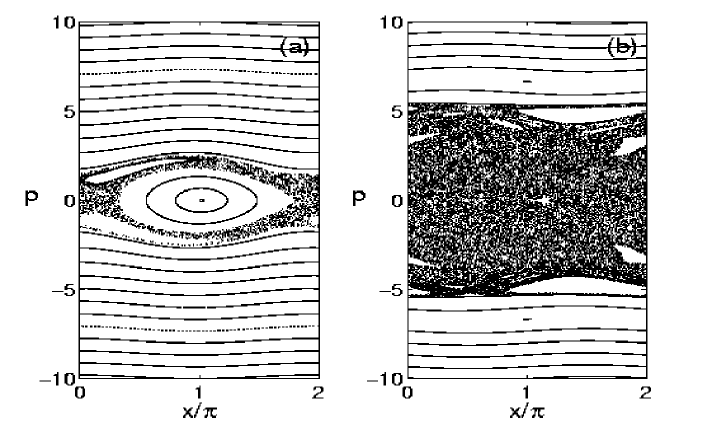
Figure 7.1: Classical stroboscopic surface of section of the system (7.1) for $F=0$. The driving frequency is $\omega=10/6$, and the amplitude $\varepsilon=0.1$ (a) and $\varepsilon=1.5$ (b). In the first case the system is almost regular, in the second case a broad chaotic band appears.

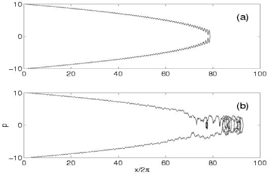
Figure 7.2: Example of classical trajectories for the system (7.1) with parameters $\omega=10/6$, $F=0.13$ and $\varepsilon=0$ (a), $\varepsilon=1.5$ (b).

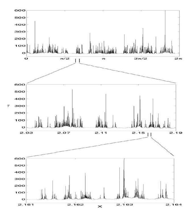
Figure 7.3: Fractal structure of the classical delay time $\tau$ as a function of the initial coordinate $x$. The system parameters are $F=0.3$, $\omega=10/6$ and $\varepsilon=1.5$.

Adding a dc field changes this property, since it destroys the invariant curves separating the chaotic component of the phase space from the outer region of the regular motion. In fact, the static field connects the regions of large momentum, because a particle initially localized in the regular region of large positive momentum $p\gg p^{*}\approx 5$ can then move into chaotic region (small momentum $|p|<p^{*}$) from where it can finally reach the region of large negative momentum. Thus the scattering process $p\rightarrow-p$ consists of tree stages: almost uniformly deaccelerated motion for $p>p^{*}$, temporal chaotic motion $|p|<p^{*}$, and accelerated motion for $p<-p^{*}$ (see Fig. 7.2). The time spent by the particle in the chaotic region is the delay or dwell time $\tau$, which we define as the time gain or loss relative the case $V(x,t)\equiv 0$

$$\tau=\lim_{p_{0}\rightarrow\infty}\left[\tau(p_{0}\rightarrow-p_{0})-2p_{0}/F\right]\,.$$ (7.3)

Figure 7.3 shows the delay time (measured in periods $T_{\omega}$) as function of the initial coordinate $x_{0}$ (the momentum $p_{0}$ is kept fixed). The function is very irregular. Regions where it is approximately constant are intermitted by regions of irregular peak structures. If we zoom into such a structure, this behavior repeats on a finer scale, and altogether the function $\tau(x_{0})$ shows a fractal behavior which is one of the main characteristics of classical chaotic scattering.

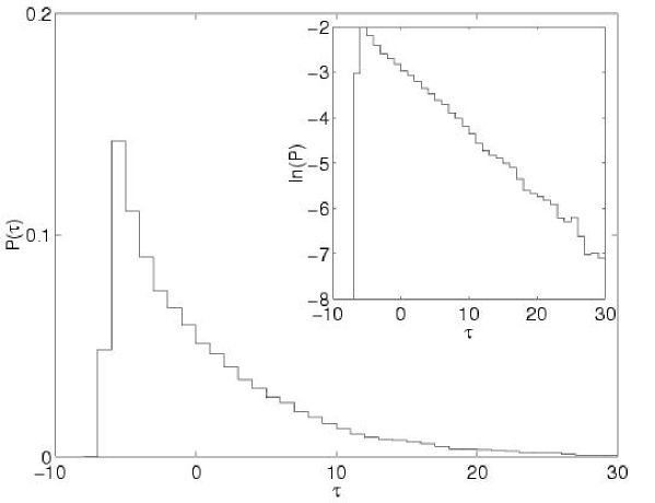
Figure 7.4: Distribution of the scaled ($\tau\rightarrow F\tau$) classical delay time for $\omega=10/6$, $\varepsilon=1.5$ and $F=0.065$.

The randomness of $\tau$ suggests its statistical analysis. Figure 7.4 shows the distribution $P_{cl}(\tau)$ of the classical delay time for $\omega=10/6$, $\varepsilon=1.5$ and $F=0.065$. It is seen that the distribution has an exponential tail

$$P_{cl}(\tau)\sim\exp(-\nu\tau)\;,$$ (7.4)

which is another characteristic feature of the chaotic scattering. The value of the decay increment $\nu$ primarily depends on $F$, and for $F=0.13$ and $F=0.065$ (used later on in the quantum simulation) it is $\nu\approx 0.13F$ or $\nu\approx 0.20F$, respectively. Note that the distribution of the delay times also defines the decay of the classical survival probability $P_{cl}(t)$. Assuming an ensemble of classical particles with initial conditions in the chaotic region, the latter quantity is defined as the relative number of particles remaining in the chaotic band. Obviously, the classical survival probability (asymptotically) decreases exponentially with the same increment $\nu$, i.e. $P_{cl}(t)\approx\exp(-\nu t)$.

7.2 Irregular quasienergy spectrum

We proceed with the quantum mechanical analysis of the system. Let us recall that we consider the commensurate case of a rational ratio between the Bloch period $T_{B}$ and the period $T_{\omega}$ of the exciting force, i.e. $T_{B}/T_{\omega}=\hbar\omega=p/q$ with integers $p$ and $q$ (see Sec. 5.1). We begin with the analysis of the complex quasienergy spectrum for the simplest case $p=q=1$, where the quasienergy spectrum coincides with the spectrum of the Floquet-Bloch operator (5.4).

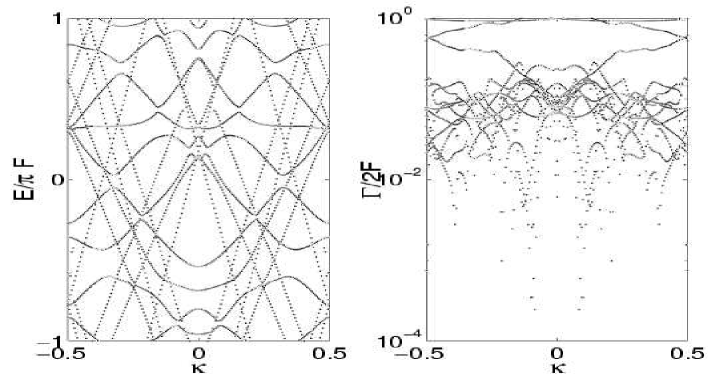
Figure 7.5: Real and imaginary parts for the quasienergy spectrum $\mathcal{E}_{\alpha}(\kappa)$ of the system (7.1) with parameters $\hbar=0.5$, $\omega=10/6$, $\varepsilon=1.5$ and $F\approx 0.13$.

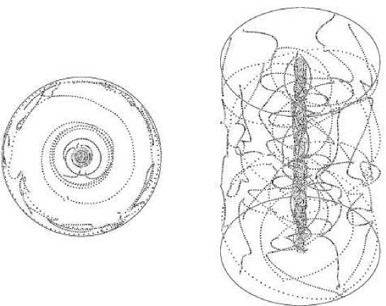
Figure 7.6: Eigenvalues $\lambda_{\alpha}(\kappa)=\exp(-{\rm i}\mathcal{E}_{\alpha}(\kappa)/F)$ in a polar plot. The left panel shows the location of the eigenvalues inside the unit circle, the right panel additionally shows the dependence on the quasimomentum.

Figure 7.5 shows the real and imaginary part of the spectrum $\mathcal{E}_{\alpha}(\kappa)$ for $\omega=10/6$, $\varepsilon=1.5$ and $\hbar=0.5$. (The value of the static force is fixed by the resonant condition $\omega=\omega_{B}=2\pi F/\hbar$, which corresponds to $F\approx 0.133$.) For each value of the quasimomentum $\kappa$, the 15 most stable resonances are plotted. In addition to Fig. 7.5, Fig. 7.6 shows the same spectrum as a polar plot for the eigenvalues $\lambda_{\alpha}(\kappa)=\exp(-{\rm i}\mathcal{E}_{\alpha}(\kappa)/F)$, where the axis of the cylinder is the quasimomentum axis. Now 30 resonances are depicted. It is seen in the figures that, apart from the symmetry $\kappa\rightarrow-\kappa$ [which reflects the symmetry $t\rightarrow-t$, $p\rightarrow-p$ of the Hamiltonian (7.1)], the spectrum looks very irregular. The formal reason for this irregularity is the interaction of the quasienergy bands discussed in Sec. 5.4. However, in the presently considered case of small $\hbar$, this interaction appears to be so strong, that it makes an analytic description of the dispersion relation impossible.

An important result following from the numerical data is a clear separation of the resonances according to their stability. Namely, for every $\kappa$ there is a finite number of relatively stable resonances which occupy the region near the unit circle in Fig. 7.6. The rest of the resonances are very unstable and they occupy the region in the center of the unit circle. Using the phase-space representation of the resonance wave function (for example the Husimi representation [161]) it can be shown that the former resonances are supported by the chaotic region of Fig. 7.1 and, thus, are associated with the chaotic component of the classical phase space. The latter resonances are associated with the outer regular region of the classical phase space and can be considered as a kind of “above-barrier” resonances. According to the Weyl rule, the total number of the relatively stable (chaotic) resonances can be estimated as

$$N=\frac{1}{2\pi\hbar}\,\oint p\,{\rm d}x\;,$$ (7.5)

where the integral $\oint p{\rm d}x$ stands for the volume of the chaotic component. Let us also note that these resonances have the width of nearly the same order of magnitude. This fact and the avoided crossings in the real part reflect the chaotic structure of the interaction region in classical phase space, which quantum mechanically results in a strong interaction of the participating states.

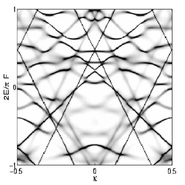
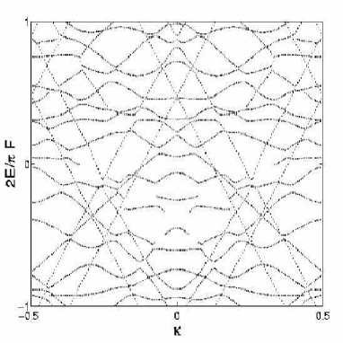
Figure 7.7: The Wigner delay time (left panel) and the real part of the quasienergy spectrum (right panel) for the system (7.1) with parameters $\varepsilon=1.5$, $\omega=10/6$ and $\hbar=0.25$ in the case $p/q=1/2$.

Additional information about the structure of the quasienergy spectrum can be obtained by considering the Wigner delay time (5.33). As an example, Fig. 7.7 shows the Wigner delay time $\tau(E)$ for $\omega/\omega_{B}=1/2$. As already mentioned in Sec. 3.4, since

$$\tau(E)\sim\sum_{\alpha}\frac{\Gamma_{\alpha}}{(E-E_{\alpha})^{2}+\Gamma_{\alpha}^{2}/4}\;,$$ (7.6)

the Wigner delay times reveals only the narrow resonances. The majority of these resonances can be identified with the chaotic resonances, which form an irregular pattern in Fig. 7.7. However, besides this irregular pattern, a regular one in the form of a rhombus is clearly seen. Below we show that this regular structure is due to the stability islands of the classical phase space.

In fact, let us consider an arbitrary term in Eq. (7.2). This term corresponds to classical nonlinear resonance at $p\approx m\omega$. Assuming that the interaction between the nonlinear resonances does not completely destroy this particular resonance, the dynamics of the system in the vicinity of its stable periodic point is locally governed by the effective Hamiltonian

$$H_{{\rm eff}}=\frac{p^{2}}{2}+J_{m}(\varepsilon)\cos(x\pm m\omega t)+Fx$$ (7.7)

(the sign of the Bessel function and the sin or cosine dependence does not matter). By substituting $x^{\prime}=x\pm m\omega t$, the Hamiltonian (7.7) is transformed to the time-independent form $H^{\prime}_{\rm eff}=(p\pm m\omega)^{2}/2+J_{m}(\varepsilon)\cos x^{\prime}+Fx^{\prime}$. The latter Hamiltonian can support localized Wannier-Stark states $\Psi_{\alpha,l}(x^{\prime})$ or, alternatively, extended Wannier-Bloch states $\Phi_{\alpha,\kappa}(x^{\prime})$. Denoting by $\mathcal{E}^{\prime}_{\alpha}$ the degenerate band of these Wannier-Bloch states, the dispersion relation for the quasienergy spectrum of the effective Hamiltonian (7.7) reads (up to an additive term)

$$\mathcal{E}_{\alpha}(\kappa)=\left\{\left(\frac{(m\omega)^{2}}{2}+\mathcal{E}^{\prime}_{\alpha}\right)\pm\kappa\,m\hbar\omega\right\}_{{\rm mod:}\hbar\omega}=\left\{\left(\frac{(m\omega)^{2}}{2}+\mathcal{E}^{\prime}_{\alpha}\right)\pm\kappa\,m2\pi F\,\frac{p}{q}\right\}_{{\rm mod:}\hbar\omega}\;.$$ (7.8)

It follows from the last equation that the nonlinear resonance index $m$ can be extracted from the slope of the dispersion lines. In particular, one can clearly identify the stability islands with $m=\pm 2$ and the remnant of the stability islands with $m=\pm 1$ in Fig. 7.1.

To summarize, the quasienergy spectrum of the Wannier-Stark system consists of two components, associated with the regular and chaotic components of the classical phase space. The “chaotic” component of the spectrum shows a rather complicated structure. This suggests a statistical analysis of the spectrum, which will be done in Sec. 7.4. Before doing this, however, we shall briefly discuss some results of random matrix theory.

7.3 Random matrix model

As was mentioned in the introductory part of this chapter, the main conjecture of random matrix theory of quantum chaos is that the spectral statistics of a classically chaotic system coincides with those of an appropriate ensemble of the random matrix. Let us first discuss which ensemble is “appropriate” to model the spectral statistics of the system of our interest.

According to the results of Sec. 5.2, the quasienergy resonances of the Wannier-Stark system are given by the eigenvalues of the nonunitary matrix (5.19), which enters in the definition of the scattering matrix (5.31). In the random matrix approach it is reasonable to keep the same structure of the matrix. In other words, we model the case of rational $\omega/\omega_{B}=p/q$ by the random scattering matrix

$$S(E)=e_{M}[B-{\rm e}^{-{\rm i}E}\leavevmode\hbox{\small 1\kern-3.8pt\normalsize 1}]^{-1}e^{M}\;,\quad e_{M}=\left(\begin{array}[]{cc}O_{N,M}&\leavevmode\hbox{\small 1\kern-3.8pt\normalsize 1}_{M,M}\end{array}\right)\;,\quad e^{M}=\left(\begin{array}[]{c}\leavevmode\hbox{\small 1\kern-3.8pt\normalsize 1}_{M,M}\\[5.69054pt] O_{N,M}\end{array}\right)\;,$$ (7.12)

where nonunitary matrix $B$ is given by

$$B=\left(\begin{array}[]{cc}O_{M,N}&O_{M,M}\\[5.69054pt] W_{N,N}&O_{N,M}\\ \end{array}\right)\;,$$ (7.13)

and $W_{N,N}$ is a random unitary matrix of size $N\times N$. In Eq. (7.12) and Eq. (7.13), the parameter $M$ is identical with the denominator $q$ in the condition of comensurability. Moreover, we choose $W_{N,N}$ to be a member of Circular Unitary Ensemble (CUE). The reason for this is that matrix $W_{N,N}$ should model the unitary matrix $\widetilde{U}^{(\kappa)}$,

$$\widetilde{U}^{(\kappa)}=\widehat{\exp}\left(-\frac{{\rm i}}{\hbar}\int_{0}^{T}{\rm d}t\,\left[\frac{(p+\hbar\kappa-Ft)^{2}}{2}+V(x,t)\right]\right)$$ (7.14)

which, excluding the cases $\kappa=0$ and $\kappa=\pm 1/2$, has no time-reversal symmetry.

Now we discuss the statistics of the resonance widths. The histograms in the left panel of Fig. 7.8 show the distribution of the scaled resonance widths for the random matrix model (7.12), (7.13) for $M=1,2,3$. These histograms are obtained in the following way. First, we generate a random $40\times 40$ GOE (Gaussian Orthogonal Ensemble) matrix, i.e., a symmetric matrix with Gaussian-distributed random elements. Then, multiplying the eigenvectors of this matrix (arranged column-wise in a square matrix) by a random-phase factor, we obtain a member of CUE [216]. This CUE matrix is enlarged to a nonunitary matrix $B$ and diagonalized. After diagonalization, we have $(N-M)$ non-zero eigenvalues $\lambda=\exp[-{\rm i}(E-{\rm i}\Gamma/2)]$. To ensure the convergence in the limit $N\rightarrow\infty$, the resonance widths $\Gamma$ are scaled based on the mean level spacing $\Delta=2\pi/(N-M)$ as $\Gamma_{s}=N\Gamma/2\approx\pi\Gamma/\Delta$. Finally, the distribution of the scaled widths is calculated for an ensemble of 1000 random matrices.

In Fig. 7.8 the distribution of the resonance widths is compared with the analytical expression

$$\Pi(\Gamma_{s})=\frac{(-1)^{M}}{(M-1)!}\,\Gamma_{s}^{M-1}\frac{{\rm d}^{M}}{{\rm d}\Gamma_{s}^{M}}\left[\frac{1-\exp(-2\Gamma_{s})}{2\Gamma_{s}}\right]\,,$$ (7.15)

valid in the limit $N\rightarrow\infty$ [217]. Note that the distribution (7.15) was originally obtained for a different random matrix model, which was aimed to model the chaotic scattering of the ballistic electrons in the mesoscopic cavities [200], and corresponds there to the so-called case of perfect coupling [199], which is realized in the case considered here. The asymptotic behavior of the distribution (7.15) is given by $\Pi(\Gamma_{s})\approx M/2\Gamma_{s}^{2}$ for $\Gamma_{s}\gg 1$, and $\Pi(\Gamma_{s})\sim\Gamma_{s}^{M-1}$ for $\Gamma_{s}\ll 1$. A perfect coincidence between the depicted numerical data and analytical results is noticed in all three considered cases.

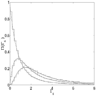
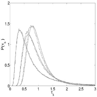
Figure 7.8: Distribution of the resonance widths (left panel) and distribution of the sum of partial delay time (right panel) for $M=1,\,2,\,3$ decay channels. Numerical data (histograms) are compared with theoretical curves (solid lines). With increasing $M$, the maxima of the distributions shift to the right.

We proceed with the distribution of the Wigner delay time. The advantage of the Wigner delay time is that it can be directly compared to classical delay time (7.3). Within the random matrix approach discussed above, the Wigner delay time can be calculated by taking the trace of the Smith matrix (5.33), where the random matrix analogue of the scattering matrix (5.31) is given in Eq. (7.12). Alternatively, we can calculate the Wigner delay time by using an $M$-channel analogue of Eq.(2.31)

$$\tau(E)=\frac{1}{M}\,{\rm Tr}\left(e^{M,{\rm t}}[B^{\dagger}-{\rm e}^{{\rm i}E}\leavevmode\hbox{\small 1\kern-3.8pt\normalsize 1}]^{-1}[B-{\rm e}^{-{\rm i}E}\leavevmode\hbox{\small 1\kern-3.8pt\normalsize 1}]^{-1}e^{M}\right)\;.$$ (7.16)

Note that the scattering matrix (7.12) yields only positive delay times whereas the Wannier-Stark system (where the delay time is compared to the “free” motion) also allows for negative values. However, we can easily take this fact into account by shifting the delay time (7.16) by $N$ units.

The distributions $P_{\rm qu}(\tau)$ of the Wigner delay times require an additional remark. The random matrix theory predicts only the distribution of the partial delay times [see Eq.(7.17) below], whereas we are interested in the Wigner delay time, which is the sum of partial delay times divided by the number of channels. Because the partial delay times are correlated, the exact distribution of the Wigner delay time is a rather complicated problem in random matrix theory [218]. However, “in the first order approximation”, the correlation of the partial delay times may be neglected. According to [219], the correlation between partial delay times decrease as $1/(M+1)$ with increasing number of scattering channels.

Then the distribution $P_{\rm qu}(\tau)$ of the Wigner delay time is the $M$-fold convolution of the distribution $P(\tau)$ for the partial delay times. According to the results of Ref. [153, 199], the latter is given by

$$P(\tau_{s})=\frac{1}{M!}\,\tau_{s}^{-M-2}\,e^{-1/\tau_{s}}\,,$$ (7.17)

where $\tau_{s}=\tau/N\approx\tau\Delta/2\pi$ is the scaled delay time.

In the right panel of Fig. 7.8, the distributions of the sum of the partial delay times are compared with the $M$-fold convolution of the distribution (7.17). An ensemble contains $1000$ random matrices of the size $40\times 40$, and for each matrix the delay time is calculated at $100$ equally spaced values of $E$. In the one channel case both results agree perfectly, whereas in the other cases the curves are slightly shifted. However, even here the agreement is pretty good. Thus, the assumption of independent partial delay times really yields a good approximation to the data.

7.4 Resonance statistics

In the previous section we introduced a random matrix model of the driven Wannier-Stark system which yields analytical results for the distribution of the resonance width and Wigner delay time. In this section we compare the actual distributions, obtained numerically, to these theoretical predictions. In our calculation, we construct the statistical ensemble by scanning the quasimomentum $\kappa$ with a step $\Delta\kappa$ over the first Brillouin zone $-1/2p\leq\kappa\leq 1/2p$. To get a good statistics, $\Delta\kappa$ should be as small as possible. On the other hand, because the widths and the delay times depend smoothly on the quasimomentum, there is a characteristic value of $\Delta\kappa$ such that a further decrease does not improve the statistics. In the following calculations we choose $\Delta\kappa=1/200p$, i.e. we average over $200$ spectra.

The other problem arising in the statistical analysis of the numerical data is the appropriate rescaling of the resonance width and the delay time. In fact, the notion of matrix size $N$ is not directly specified in our approach. However, we can use the semiclassical estimate (7.5) to specify the parameter $N$. For the value of the scaled Plank constant $\hbar=0.25$ considered below this gives $N\approx 32$. In what follows, however, we use a slightly smaller value $N=28$ which accounts for the embedded islands of stability.

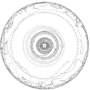
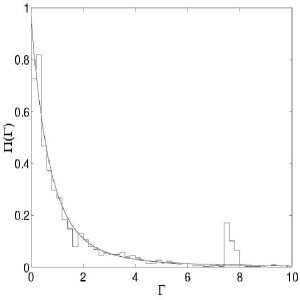
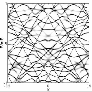
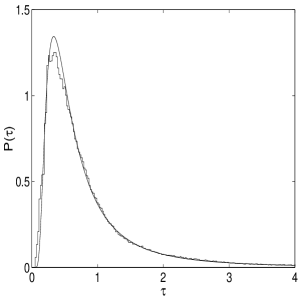
Figure 7.9: Complex quasienergies, distribution of the widths, delay time and distribution of the delay times of the system (7.1) for the case $p/q=1$ with parameters $\varepsilon=1.5$, $\omega=10/6$ and $\hbar=0.25$. In this case the constant force is $F\approx 0.066$.

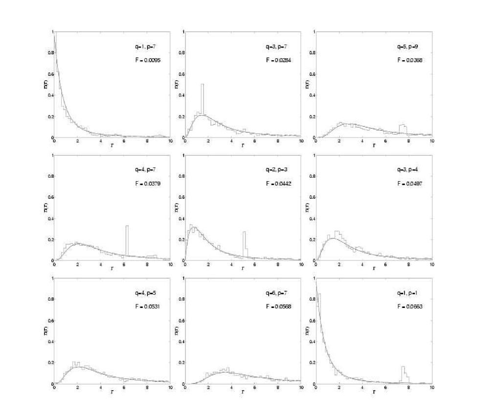
Figure 7.10: Distribution of the resonance widths for different field strengths $F$ with $\varepsilon=1.5$, $\omega=10/6$ and $\hbar=0.25$. The histogram show the numerical data, the solid lines are the random matrix predictions (7.15) for the proper number of decay channels.

The two upper panels of Fig. 7.9 show the complex quasienergies and the distribution of the resonance widths for the most simple single channel case $p=q=1$. A good agreement between the random matrix results and the calculated distribution is noticed. The distribution has its maximum at $\Gamma_{s}=0$, i.e. the resonances tend to be long-lived. The main deviation is a peak at $\Gamma_{s}\approx 8$, which is due to states associated with stability islands in the classical surface of section. One also finds these resonances in the delay time shown in the left lower panel of Fig. 7.9. As discussed in Sec. 7.2, resonances corresponding to classical stability islands form straight lines in the quasienergy spectrum. Indeed, we can see the lines with the slope $\pm 4\pi$ and remnants of two lines with slope $\pm 2\pi$. Because such resonances have approximately the same widths, their signatures are easily identified in the distribution of the widths.

The right lower panel shows the distribution of the delay time (to facilitate the comparison, the histogram for the scaled delay time is shifted to the right by one unit.) Here the agreement is pretty good, either. The location of the maxima at $\tau_{s}=0.33$ and the shape of both distributions coincide almost perfectly.

We proceed with the case $p/q\neq 1$, where we restrict ourselves to an analysis of the resonance widths. The most striking prediction of the random matrix model of Sec. 7.3 is that the statistics of the resonance widths is solely defined by the integer $q$. On the other hand, the random matrix model is supposed to describe the properties of the real system with four parameters. Thus, provided $q$ is the same, the distribution of the resonance widths should be independent on the particular choice of the other system parameters. (Of course, the condition for chaotic dynamics should be fulfilled.) To check this prediction we proceed as follows.

The number $q$ of decay channels is defined by the rationality condition $pT_{\omega}=qT_{B}$, i.e. in terms of the system parameters by $F=q\hbar\omega/p2\pi$. As in the preceding cases, we choose $\varepsilon=1.5$ and $\omega=10/6$ to ensure that the system is classically chaotic, and $\hbar=0.25$ in order to be in the semiclassical regime. Then we calculate the distribution of the resonance widths for several combinations of the integers $p$ and $q$, which correspond to increasing values of $F$. Naively one would expect that with increasing $F$ the resonances tend to destabilize. Instead the distributions follow closely the RMT distributions for the $q$-channel case as can be seen in Fig. 7.10. The first and the last picture for the smallest and the largest field strength correspond to the one-channel case $q=1$. Note that the field strength differs by a factor seven, but the distributions are essentially the same. For the intermediate field strengths the distributions vary according to the number of decay channels. We should stress that the only adjusted parameter, the number of states $N=28$ defining the scaled width $\Gamma_{s}$, is constant in all figures.

7.5 Fractional stabilization

In this section we discuss an interesting application of the results of preceding section, which can be referred to as fractional stabilization of the Wannier-Stark system.

Let us discuss again the spectroscopic experiment [123], where the survival probability for the cold atoms in the accelerated optical lattice was measured as a function of the driving frequency (see Sec. 4.3).We assume now the following modifications of the experimental setup. The value of the scaled Planck constant (which is inversely proportional to the laser intensity) is small enough to insure the semiclassical dynamics of the system. The value of the driving amplitude is large enough to guarantee the classical chaotic dynamics of the atoms. (Note that both these condition were satisfied in a different experiment [221].) The atomic survival probability is measured as a function of the acceleration but not as the function of the driving frequency, i.e. we vary $\omega_{B}$ instead of varying $\omega$. (This condition is actually optional.)

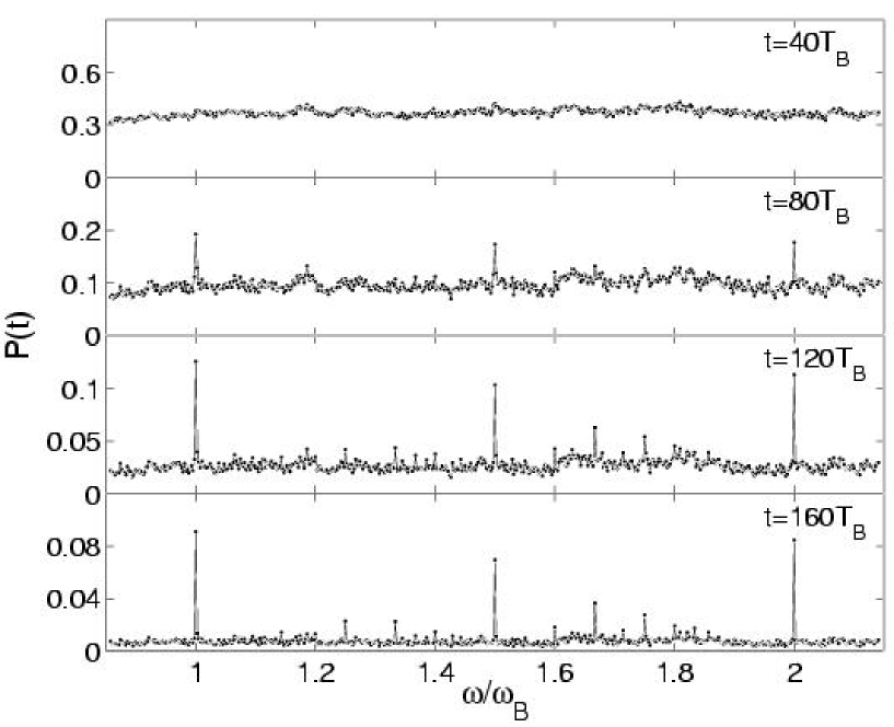
Figure 7.11: Survival probability as function of the control parameter $\gamma=\omega/\omega_{B}$. The system parameters are $\omega=10/6$, $\varepsilon=1.5$ and $\hbar=0.25$.

Figure 7.11 shows the results of the numerical calculation of the quantum survival probability $P_{\rm qu}(t)$ based on direct numerical simulation of the wave packet dynamics. The survival probability shows an interesting behavior. For small times, the curve fluctuates around an approximately constant value. When the time is increased, this average value decreases exponentially. In addition, however, peaks develop at integer values $\gamma=\omega/\omega_{B}$ and, incrementally, at rational $\gamma=p/q$ with small denominator. Thus, the decay is slowed down for rational $\gamma$. In what follows we explain this stabilization effect by using RMT approach.

Indeed, the system parameters were chosen to ensure the regime of chaotic scattering. Then the distribution of the resonance widths is given by equation (7.15). Let us assume that the initial state uniformly populates all resonances. If we then neglect the overlap of the resonances (this is the so-called diagonal approximation) the survival probability is given by the integral [220]

$$P_{\rm qu}(t)=\int_{0}^{\infty}{\rm d}\Gamma\,\Pi(\Gamma)\,{\rm e}^{-\Gamma t/\hbar}\,,$$ (7.18)

where $\Gamma=2\Gamma_{s}/N$ and $N$ is the number of states in the interaction region. The long-time asymptotics of this integral is defined by the behavior of $\Pi(\Gamma)$ at small $\Gamma$, where it increases as the power law $\Pi(\Gamma)\sim\Gamma^{q-1}$. Consequently, the survival probability asymptotically follows the inverse power law $P_{\rm qu}(t)\sim t^{-q}$. Thus, the asymptotics depend on the number of decay channels and therefore on the denominator of the control parameter $\gamma=\omega/\omega_{B}=p/q$.

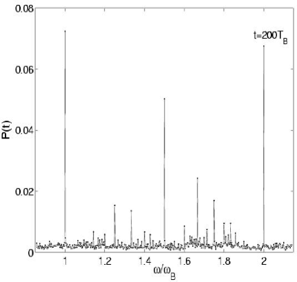
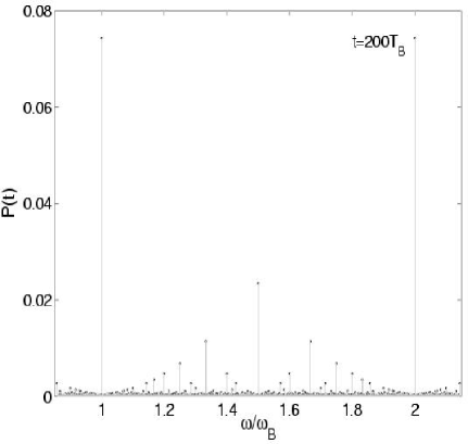
Figure 7.12: Survival probability at $t=200T_{B}$. The left part shows the numerical data, the right part the theoretical curve based on equation (7.19). To stress the discontinuous character of the latter function, we slightly changed its graphical representation.

With the help of supersymmetric techniques, $P_{\rm qu}(t)$ can be calculated beyond the diagonal approximation. This gives more elaborated result [220]

$$P_{\rm qu}(t)\approx\left(1+\frac{\Gamma_{W}t}{\hbar q}\right)^{-q}\;.$$ (7.19)

where $\Gamma_{W}$ is the so-called Weisskopf width (which is a free parameter in the abstract random matrix theory). For rational $\gamma$ and large times the decay of the survival probability is algebraic, $P_{\rm qu}(t)\sim t^{-q}$, as found in the diagonal approximation. The case of irrational $\gamma$ can be approximated by the limit $q\rightarrow\infty$. Then the system shows the exponential decay, $P_{\rm qu}(t)=\exp(-\Gamma_{W}t/\hbar)$ and its natural to identify the parameter $\Gamma_{W}/\hbar$ with the classical decay coefficient $\nu$.

The right panel in Fig. 7.12 shows the values of the function (7.19) for $t=200\,T_{B}$ and some rational values of $\gamma=\omega/\omega_{B}$. Here we use a slightly different graphic presentation of $P_{\rm qu}(t)$ to stress that the function (7.19) is a discontinuous function of $\gamma$ for any $t$. In contrast, the atomic survival probability shown in the left panel is a continuous function of $\gamma$ where its discontinuous structure develops gradually as $t\rightarrow\infty$. In fact, the survival probabilities calculated for two close rational numbers $\gamma_{1}$ and $\gamma_{2}$ follow each other during a finite “correspondence” time. (For instance, for $\gamma_{1}=1$ and $\gamma_{2}=999/1000$ the correspondence time is found to be about $50\,T_{B}$.) Thus it takes some time to distinguish two close rationals, although they may have very different denominators and, therefore, very different asymptotics. With this remark reserved, a nice structural (and even semiquantitative) correspondence is noticed.

The described numerical experiment suggest a simple laboratory experiment with cold atoms in optical lattice, where one can test the statistics of the resonance width indirectly, by measuring the survival probability for atoms.

Chapter 8 Conclusions and outlook

In this section we review the main results of the work and outline some problems which are still waiting for their solutions. In the overview we shall mainly follow the table of contents.

The approach introduced in Sec. 2 gives us a powerful tool for analyzing an arbitrary one-dimensional Wannier-Stark system, i.e. a system with potential energy given by the sum of periodic and linear terms. The success of the method is ensured by two key points. First, we inverted the traditional solid state approach, where the linear term has been treated as “a perturbation” to the periodic term, and formulate the problem as scattering of a quantum particle by a periodic potential. Second, instead of dealing with the Hamiltonian, we work with the evolution operator. Although both these points were discussed earlier, it is only a combination of them, which provides solution of the Wannier-Stark problem. Let us also note that the use of the evolution operator provides a way to an analysis of the Wannier-Stark system affected additionally by a time-periodic perturbation. The corresponding generalization of the method, which leads to the notion of the metastable quasienergy Wannier-Stark states, is discussed in Sec. 5 of this review.

We apply the developed theory to analyze the Wannier-Stark ladder of resonances in two particular systems – undoped semiconductor superlattices in a static electric field and the system of cold atoms in optical lattices in an accelerated frame. Both of these systems mimic the crystal electron in a static electric field (which was the original formulation of the problem) and have their own advantages and disadvantages. In particular, the semiconductor superlattices allow (at least, in principle) to create an arbitrary periodic potential. One may think, for example, about a periodic sequence of double wells, where the interaction of the Wannier-Stark ladders (which is essentially the resonance tunneling effect) should have an especially interesting form. In Sec. 3 we restricted ourselves by considering the cosine and square-box shaped potentials. The structure of the Wannier-Stark states and the interaction of the ladders in periodic potentials of a different form (like the already mentioned double-well array or asymmetric ratchet-like potential) is an open problem.

A disadvantage of the semiconductor superlattice is that this is a more “dirty” (in comparison with the optical superlattice) system, where the effects in question interfere with other effects like electron-hole Coulomb interaction, scattering by impurities, etc. Nevertheless, if we want to move further, we should learn how to deal with these complications. In the first turn, the effect of Coulomb interaction should be taken into account. We believe that now this problem can be solved rigorously by extending the one-particle scattering theory of Sec. 2 to the case of two particles.

We turn to the spectroscopic results of Sec. 4. In this section we derive an analytic expression for the decay spectrum of the system of cold atoms in an optical lattice and the absorption spectrum of semiconductor superlattices. This expression involves complex valued squared transition matrix elements (non-real squared matrix elements appear because of the resonance nature of the Wannier-Stark states), which lead to a non-Lorentzian shape of the absorption lines. Although the relation of these results to the famous Fano theory is obvious, the details of this relation remain unexplored.

The brief Sec. 6 was inspired by the experiment of Anderson and Kasevich, where a pulsed output from the periodic array of cold atoms was observed. We give a proper theoretical description of this phenomenon which, in fact, is the Bloch oscillations in the case of a strong static field. In this sense, Sec. 6 is the only section of the review discussing Bloch oscillations. One might be interested in other regimes of Bloch oscillations. Evolution of the theory in this direction is reflected by a recent paper [222].

As already mentioned in the introduction, Sec. 7 deals with the very different problem of chaotic scattering, which is primary of interest to the members of quantum chaos community. Nevertheless, from the formal point of view, the results of Sec. 7 are just the results beyond the perturbative approach of Sec. 5. Thus, when the experimentalists overcome the perturbation limit (the present state of the art), Sec. 7 may change its status from of “pure theoretical interest” to that of “practical importance”.

To conclude, we would like to highlight one more problem. This work is devoted entirely to one-dimensional Wannier-Stark systems. However, practically nothing is known about the Wannier-Stark states in 3D- or 2D-lattices (a first step in this direction was taken only recently [223]). An extension of the present theory to higher dimension is of much theoretical and practical interest and one may expect on this way a variety of new phenomena which are absent in the one-dimensional case.

Furthermore, the results presented in this review will also be relevant in connection with recent new developments in quantum transport in driven periodic lattices with broken symmetry, i.e. quantum hamiltonian ratchets [224, 225, 226, 227, 228].  Such ratchets are usually studied in the case of vanishing mean potential gradient. An interesting situation arises, e.g., for ratchets inclined in the direction opposed to the current that would occur in the unbiased case.  In addition, it should be noted that in the previous studies of the classical – quantum correspondence for driven Wannier–Stark systems as discussed in Sec. 7, the parameters have been chosen to guarantee (almost) fully chaotic dynamics in the scattering region, i.e. classical stability islands are of minor importance. Larger islands can be observed, however, and will certainly effect the decay properties discussed in Sec. 7, as for instance by chaos–assisted tunneling, a topic of much interest in theoretical [229, 230, 231] and very recently also experimental studies [232, 233, 234], were this phenomenon was rediscovered.

Acknowledgments

The authors gratefully acknowledge the support of the Deutsche Forschungsgemeinschaft via the Schwerpunktprogramm SSP 470 “Zeitabhängige Phänomene und Methoden in Quantensystemen der Physik und Chemie” as well as the Graduiertenkolleg “Laser- und Teilchenspektroskopie”. Stimulating discussions with many colleagues are gratefully acknowledged, in particular, among others, with J. E. Avron, Y. V. Fyodorov, M. Holthaus, K. Leo, N. Moiseyev, Q. Niu, M. G. Raizen, D. V. Savin, V. V. Sokolov, and K. Zyczkowski. It is also a pleasure to thank the graduate students Michael Hankel, Christian Hebell, Frank Keck, Stefan Mossmann, Frank Zimmer who contributed to our studies of Wannier-Stark systems. Moreover, we thank P. Hänggi for many useful suggestions which considerably improved the present review.

Bibliography

- [1] F. Bloch, Über die Quantenmechanik der Electronen in Kristallgittern, Z. Phys 52 (1928) 555
- [2] C. Zener, A Theory of Electrical Breakdown of Solid Dielectrics, Roy. Soc. Lond. A 145 (1934) 523
- [3] G. H. Wannier, Wave Functions and Effective Hamiltonian for Bloch Electrons in an Electric Field, Phys. Rev. 117 (1960) 432
- [4] J. Zak, Stark Ladder in Solids?, Phys. Rev. Lett. 20 (1968) 1477
- [5] G. H. Wannier, Stark Ladder in Solids? A Reply, Phys. Rev. 181 (1969) 1364
- [6] J. Zak, Stark Ladder in Solids? A Reply to a Reply, Phys. Rev. 181 (1969) 1366
- [7] A. Rabinovitch and J. Zak, Electrons in Crystals in Finite-Range Electric Fields, Phys. Rev. B 4 (1971) 2358
- [8] W. Shockley, Stark Ladders for Finite, One-Dimensional Models of Crystals, Phys. Rev. Lett. 28 (1972) 349
- [9] A. Rabinowitch and J. Zak, Does a Bloch Electron in a Constant Electric Field Oscillate?, Phys. Lett. A 40 (1972) 189
- [10] J. N. Churchill and F. E. Holmstrom, Comments on the Existence of Bloch Oscillations, Phys. Lett. A 85 (1981) 453
- [11] J. N. Churchill and F. E. Holmstrom, Energy States and Bloch States for an Accelerated Electron in a Periodic Lattice, Phys. Scripta 27 (1983) 91
- [12] J. B. Krieger and G. J. Iafrate, Time Evolution of Bloch Electrons in a Homogeneous Electric Field, Phys. Rev. B 33 (1986) 5494
- [13] D. Emin and C. F. Hart, Existence of Wannier-Stark Localization, Phys. Rev. B 36 (1987) 7353
- [14] C. F. Hart and D. Emin, Time evolution of a Bloch electron in a constant electric field, Phys. Rev. B 37 (1988) 6100
- [15] L. Kleinman, Comment on ”Existence of Wannier-Stark localization”, Phys. Rev. B 41 (1990) 3857
- [16] J. Zak, Comment on the existence proofs of the Wannier-Stark ladder, Phys. Rev. B 43 (1991) 4519
- [17] D. A. Page and E. Brown, Comment on ”Existence of Wannier-Stark localization”, Phys. Rev. B 43 (1991) 2423
- [18] J. Leo and A. MacKinnon, Comment on ”Existence of Wannier-Stark localization”, Phys. Rev. B 43 (1991) 5166
- [19] X. G. Zhao, Bloch Electron in a Uniform Electric Field, Phys. Rev. B 46 (1992) 1305
- [20] G. Nenciu, Dynamics of band electrons in electric and magnetic fields: rigorous justification of the effective Hamiltonians, Rev. Mod. Phys. 63 (1991) 91
- [21] A. M. Bouchard and M. Luban, Bloch Oscillations and other Dynamical Phenomena of Electrons in Semiconductor Superlattices, Phys. Rev. B 52 (1995) 5105
- [22] F. Rossi, Bloch Oscillations and Wannier-Stark Localization in Semiconductor Superlattices, in E. Schöll, editor, Theory of Transport Properties of Semiconductor Nanostructures, page 283. Chapman & Hall, London, 1998
- [23] J. E. Avron, J. Zak, A. Grossmann, and L. Gunther, Instability of the continuous spectrum: The N-band Stark ladder, J. Math. Phys. 18 (1977) 918
- [24] F. Bentosela, R. Carmona, P. Duclos, B. Simon, B. Souillard, and R. Weder, Schrödinger Operators with an Electric Field and Random or Deterministic Potentials, Com. Math. Phys. 88 (1983) 387
- [25] I. W. Herbst and J. S. Howland, The Stark Ladder and Other One-Dimensional External Field Problems, Com. Math. Phys. 80 (1981) 23
- [26] J. Agler and R. Froese, Existence of Stark Ladder Resonances, Com. Math. Phys. 100 (1985) 161
- [27] J.-M. Combes and P. D. Hislop, Stark Ladder Resonances for Small Electric Fields, Com. Math. Phys. 140 (1991) 291
- [28] F. Bentosela and V. Grecchi, Stark Wannier Ladders, Com. Math. Phys. 142 (1991) 169
- [29] N. Moiseyev, Quantum theory of resonances: calculating energies, widths and cross-sections by complex scaling, Phys. Rep. 302 (1998) 211
- [30] J. E. Avron, Model Calculations of Stark Ladder Resonances, Phys. Rev. Lett. 37 (1976) 1568
- [31] J. E. Avron, The Lifetime of Wannier Ladder States, Ann. Phys. (N.Y.) 143 (1982) 33
- [32] V. Grecchi, M. Maioli, and A Sacchetti, Wannier Ladders and Perturbation Theory, J. Phys. A 26 (1993) L379
- [33] V. Grecchi, M. Maioli, and A Sacchetti, Stark Ladder of Resonances: Wannier Ladders and Perturbation Theory, Com. Math. Phys. 159 (1994) 605
- [34] V. Grecchi and A. Sacchetti, Crossing and Anticrossing of Resonances: The Wannier-Stark Ladders, Ann. Phys. (N.Y.) 241 (1995) 258
- [35] V. Grecchi and A. Sacchetti, Metastable Bloch Oscillators, Phys. Rev. Lett. 78 (1997) 4474
- [36] V. Grecchi and A. Sacchetti, Lifetime of the Wannier-Stark Resonances and Parturbation Theory, Com. Math. Phys. 185 (1997) 359
- [37] V. Grecchi and A. Sacchetti, Wannier-Bloch Oscillators, Com. Math. Phys. 197 (1998) 553
- [38] V. Buslaev and A. Grigis, Imaginary Parts of Stark-Wannier Resonances, J. Math. Phys. 39 (1998) 2520
- [39] J. Banavar and D. D. Coon, Widths and Spacing of Stark Ladder Levels, Phys. Rev. B 17 (1978) 3744
- [40] F. Bentosela, V. Grecchi, and F. Zironi, Approximate ladder of resonances in a semi-infinite crystal, J. Phys. C: Solid State Phys. 15 (1982) 7119
- [41] F. Bentosela, V. Grecchi, and F. Zironi, Oszillations of Wannier Resonances, Phys. Rev. Lett. 50 (1983) 84
- [42] M. Ritze, N. J. M. Horing, and R. Enderlein, Density of States and Wannier-Stark Levels of Superlattices in an Electric Field, Phys. Rev. B 47 (1993) 10437
- [43] M. C. Chang and Q. Niu, Local density of states and level width for Wannier-Stark ladders, Phys. Rev. B 48 (1993) 2215
- [44] C. L. Roy and P. K. Mahapatra, Bloch electrons in finite crystals in the presence of a uniform electric field, Phys. Rev. B 25 (1982) 1046
- [45] B. Soucail, R. Ferreira, G. Bastard, and P. Voisin, Instability of Energy Band Structure at Low Electric Field: Numerical Analysis of Superlattice Minibands, Europhys. Lett. 15 (1991) 857
- [46] B. Mendez and F. Dominguez-Adame, Stark Ladders in Periodically Si--Doped GaAs, Phys. Rev. B 49 (1994) 11471
- [47] S. Glutsch and F. Bechstedt, Interaction of Wannier-Stark Ladders and Electrical Breakdown in Superlattices, Phys. Rev. B 60 (1999) 16584
- [48] H. Fukuyama, R. A. Bari, and H. C. Fogedby, Tightly Bound Electrons in a Uniform Electric Field, Phys. Rev. B 8 (1973) 5579
- [49] D. H. Dunlap and V. M. Kenkre, Dynamic localization of a charges particle moving under the influence of an electric field, Phys. Rev. B 34 (1986) 3625
- [50] X.-G. Zhao, Dynamic Localization Conditions of a Charged Particle in a dc-ac Electric Field, Phys. Lett. A 155 (1991) 299
- [51] X.-G. Zhao, Motion of Bloch Electrons in Time-Dependent Electric Fields with Off-Diagonal Effects, Phys. Lett. A 167 (1992) 291
- [52] N. Hhong-Shon and H. N. Nazareno, J. Phys. Cond. Matter 4 (1992) L611
- [53] X.-G. Zhao and Q. Niu, Localization of Band Electrons in dc-ac Electric Fields, Phys. Lett. A 191 (1994) 181
- [54] X.-G. Zhao, R. Jahnke, and Q. Niu, Dynamic Fractional Stark Ladders in dc-ac Fields, Phys. Lett. A 202 (1995) 297
- [55] K. Drese and M. Holthaus, Exploring a Metal-Insulator Transition with Ultracold Atoms in Standing Light Waves?, Phys. Rev. Lett. 78 (1997) 2932
- [56] M. Grifoni and P. H. Hänngi, Driven Quantum Tunneling, Phys. Rep. 304 (1998) 229
- [57] D. W. Hone and M. Holthaus, Locally Disordered Lattices in Strong Ac Electric Fields, Phys. Rev. B 48 (1993) 15123
- [58] H. Yamada, K. Ikeda, and M. Goda, Quantum diffusion in a coherently time-varying one-dimensional disordered system, Phys. Lett. A 182 (1993) 77
- [59] M. Holthaus, G. H. Ristow, and D. W. Hone, ac-Field-Controlled Anderson Localization in Disordered Semiconductor Superlattices, Phys. Rev. Lett. 75 (1995) 3914
- [60] M. Holthaus, G. H. Ristow, and D. W. Hone, Random lattices in combined ac and dc electric fields: Anderson vs. Wannier-Stark localization, Europhys. Lett. 32 (1995) 241
- [61] K. Drese and M. Holthaus, Anderson Localization in an ac-Driven Two-Band Model, J. Phys. Condens. Matter 8 (1996) 1193
- [62] H. Yamada, K. S. Ikeda, Anomalous diffusion and scaling behavior of dynamically perturbed one-dimensional disordered quantum systems, Phys. Lett. A 248 (1993) 179
- [63] D. Suqing and X.-G. Zhao, Effect of External Noise on Dynamic Localization of a Charged Particle, Phys. Rev. B 61 (2000) 5442
- [64] V. I. Kovanis and V. M. Kenkre, Exact Self-Propagators for Quasiparticle Motion on a Chain with Alternating Site Energies or Intersite Interactions, Phys. Lett. A 130 (1988) 147
- [65] X.-G. Zhao, Exact Solutions for a Charged Particle in a Uniform Electric Field with Alternating Site Energies: Perturbation Theory, J. Phys.: Condens. Matter 3 (1991) 6021
- [66] X.-G. Zhao, Dynamics of a Periodic Binary Sequence in an AC Field, J. Phys.: Condens. Matter 9 (1997) L385
- [67] S.-Q. Bao, X.-G. Zhao, X.-W. Zhang, and W.-X. Yan, Dynamics of a Charged Particle on a Periodic Binary Sequence in an External Field, Phys. Lett. A 240 (1998) 7771
- [68] P. H. Rivera and P. A. Schulz, Tuning of Dynamic Localization in Coupled Minibands: Signatures of a Field-Induced Metal-Insulator Transition, Phys. Rev. B 61 (2000) R7865
- [69] J. Rotvig, A.-P. Jauho, and H. Smith, Bloch Oscillations, Zener Tunneling and Wannier-Stark Ladders in the Time Domain, Phys. Rev. Lett. 74 (1995) 1831
- [70] J. Rotvig, A.-P. Jauho, and H. Smith, Theory of coherent time-dependent transport in one-dimensional multiband semiconductor superlattices, Phys. Rev. B 54 (1996) 17691
- [71] D. W. Hone and X.-G. Zhao, Time-periodic behaviour of multiband superlattices in static electric fields, Phys. Rev. B 53 (1996) 4834
- [72] X.-G. Zhao, W.-X. Yan, and D. W. Hone, Zener transitions between dissipative Bloch bands, Phys. Rev. B 57 (1998) 9849
- [73] W.X. Yan, X.-G. Zhao, and S.-Q. Bao, Dynamics of two-band semiconductor superlattices driven by static and time-dependent fields, Physica B 252 (1998) 63
- [74] X.-G. Zhao, G. A. Georgakis, and Q. Niu, Rabi oscillations between Bloch bands, Phys. Rev. B 54 (1996) R5235
- [75] W. Kohn, Construction of Wannier Functions and Applications to Energy Bands, Phys. Rev. B 7 (1972) 4388
- [76] W. Kohn, Analytic Properties of Bloch Waves and Wannier Functions, Phys. Rev. 115 (1959) 809
- [77] G. Nenciu, Existence of the Exponentially Localized Wannier Functions, Com. Math. Phys. 91 (1983) 81
- [78] W. V. Houston, Acceleration of Electrons in a Crystal lattice, Phys. Rev. 57 (1940) 184
- [79] L. D. Landau, Phys. Z. Sov. 1 (1932) 46
- [80] R. W. Koss and L. M. Lambert, Experimental Observation of Wannier Levels in Semi-Insulating Gallium Arsenide, Phys. Rev. B 5 (1972) 1479
- [81] L. Esaki, The Evolution of Semiconductor Quantum Structures. Do-It-Yourself Quantum Mechanics,, in A. Stella and L. Miglio, editors, Superreticoli e Interface die Semiconduttori, number 117 in Proceedings of the International School of Physics ”Enrico Fermi”, page 1, Amsterdam, 1993. North-Holland
- [82] E. E. Mendez, F. Agullo-Rueda, and J. M. Hong, Stark Localizations in GaAs-GaAlAs Superlattices under an Electric field, Phys. Rev. Lett. 60 (1988) 2426
- [83] P. Voisin, J. Bleuse, C. Bouche, S. Gaillard, C. Alibert, and A. Regreny, Observation of the Wannier-Stark quantization in a semiconductor superlattice, Phys. Rev. Lett. 61 (1988) 1639
- [84] E. E. Mendez and G. Bastard, Wannier-Stark Ladders and Bloch Oscillations in Superlattices, Physics Today 46(6) (1993) 34
- [85] J. Feldmann, K. Leo, J. Shah, B. A. B. Miller, J. E. Cunningham, T. Meier, G. von Plessen, A. Schulze, P. Thomas, and S. Schmitt-Rink, Optical Investigation of Bloch Oscillations in a Semiconductor Superlattice, Phys. Rev. B 46 (1992) 7252
- [86] K. Leo, P. H. Bolivar, F. Brüggemann, R. Schwedler, and K. Köhler, Observation of Bloch Oscillations in a Semiconductor Superlattice, Solid State Comm. 84 (1992) 943
- [87] G. von Plessen and P. Thomas, Method for Observing Bloch Oscillations in the Time Domain, Phys. Rev. B 45 (1992) 9185
- [88] C. Waschke, H. G. Roskos, R. Schwedler, K. Leo, H. Kurz, and K. Köhler, Coherent Submillimeter-Wave Emission from Bloch Oscillations in a Semiconductor Superlattice, Phys. Rev. Lett. 70 (1993) 3319
- [89] T. Dekorsy, P. Leisching, K. Köhler, and H. Kurz, Electro-Optic Detection of Bloch Oscillations, Phys. Rev. B 50 (1994) 8106
- [90] G. C. Cho, T. Dekorsy, H. J. Bakker, H. Kurz, A. Kohl, and B. Opitz, Bloch-Oscillations in In-Ga-As-P/In-Ga-As-P Heterostructures Oberved with Time-Resolved Transmission Spectroscopy, Phys. Rev. B 54 (1996) 4420
- [91] K. Leo, Interband Optical Investigation of Bloch Oscillations in Semiconductor Superlattices, Semicond. Sci. Technol. 13 (1998) 249
- [92] T. Dekorsy, R. Ott, and H. Kurz, Bloch Oscillations at Room Temperature, Phys. Rev. B 51 (1995) 17275
- [93] V. G. Lyssenko, G. Valusis, F. Löser, T. Hasche, and K. Leo, Direct Measurement of the Spatial Displacement of Bloch-Oscillating Electrons In Semiconductor Superlattices, Phys. Rev. Lett. 79 (1997) 301
- [94] M. Sudzius, V. G. Lyssenko, F. Löser, K. Leo, M. M. Dignam, and K. Köhler, Optical Control of Bloch-Oscillation Amplitudes: From Harmonic Spatial Motion to Breathing Modes, Phys. Rev. B 57 (1998) R12693
- [95] B. Soucail, N. Dupuis, R. Ferreira, P. Voisin, A. P. Roth, D. Morris, K. Gibb, and C. Lacelle, Electron Minibands and Wannier-Stark Quantization in an In0.15Ga0.85As-GaAs Strained-Layer Superlattice, Phys. Rev. B 41 (1990) 8568
- [96] D. M. Whittaker, M. S. Skolnick, G. W. Smith, and C. R. Whitehouse, Wannier-Stark Localization of and States in GaAs-AlAs Short-Period Superlattices, Phys. Rev. B 42 (1990) 3591
- [97] H. Schneider, K. Jawashima, and K. Fujiwara, Stark Localization of a Pair of Coupled Minibands in GaAs/AlAs Double-Period Superlattice, Phys. Rev. B 44 (1991) 5943
- [98] R. H. Yu, Wannier-Stark Localization in Modulation-Doped Multiple-Quantum-Well Structures, Phys. Rev. B 49 (1994) 4673
- [99] D. W. Peggs, M. S. Skolnik, D. M. Whittaker, R. A. Hogg, A. R. K. Willcox, D. J. Mowbray, R. Grey, G. J. Rees, L. Hart, M. Hopkinson, G. Hill, and M. A. Pate, Observation of Wannier-Stark Ladder Transitions in InxGa1-xAs-GaAs Piezoelectric Superlattices, Phys. Rev. B 52 (1995) R14340
- [100] K. Gibb, M. M. Digman, J. E. Sipe, and A. P. Roth, Observation of Wannier-Stark Localization by Electroreflectance Spectroscopy, Phys. Rev. B 48 (1993) 8156
- [101] C. Hamaguchi, M. Yamaguchi, M. Morifuji, H. Kubo, K. Taniguchi, C. Gmachl, and E. Gornik, Wannier-Stark Effect in Superlattices, Semicond. Sci. Technol. 9 (1994) 1994
- [102] H. Schneider, H. T. Grahn, K. v. Klitzing, and K. Ploog, Resonance-Induced Delocalization of Electrons in GaAs-AlAs Superlattices, Phys. Rev. Lett. 65 (1990) 2720
- [103] M. Nakayama, I. Tanaka, H. Nishimura, K. Kawashima, and K. Fujiwara, Electroreflectance Detection of Resonant Coupling between Wannier-Stark Localization States in Semiconductor Superlattices, Phys. Rev. B 44 (1991) 5935
- [104] I. Tanaka, M. Nakayama, H. Nishimure, K. Kawashime, and K. Fujiwara, Electroreflectance Intensity for Resonant Coupling between Wannier-Stark Localisation States in GaAs/AlAs Superlattice, Phys. Rev. B 46 (1992) 7656
- [105] G. Bastard, R. Ferreira, S. Chelles, and P. Voisin, Interaction between Wannier-States in Semiconductor Superlattices, Phys. Rev. B 50 (1994) 4445
- [106] H. Kümmel, R. Till, and A. Philip, Photocurrent Spectroscopy of Low-Electric-Field Anticrossings in Semiconductor Superlattices, Phys. Rev. B 60 (1999) 4470
- [107] G. von Plessen, T. Meier, J. Feldmann, E. O. Göbel, P. Thomas, K. W. Goossen, J. M. Kuo, and R. F. Kopf, Influence of Scattering on the Formation of Wannier-Stark Ladders and Bloch-Oscillations in Semiconductor Superlattices, Phys. Rev. B 49 (1994) 14058
- [108] J.-B. Xia, Scattering Rates of Wannier States in Superlattices in an Electric Field, Phys. Rev. B 50 (1994) 15067
- [109] F. Löser, Y. A. Kosevich, K. Köhler, and K. Leo, Dynamics of Bloch Oscillation under the Influence of Scattering and Coherent Plasmon Coupling, Phys. Rev. B 61 (2000) R13373
- [110] E. Ribeiro, F. Cerdeira, and A. P. Roth, Step-by-Step Evolution from Franz-Keldysh Oscillations to Wannier-Stark confinement in an In0.12Ga0.88/GaAs Superlattice, Phys. Rev. B 46 (1992) 12542
- [111] K. H. Schmidt, N. Linder, G. H. Döhler, H. T. Grahn, K. Ploog, and H. Schneider, Coexistence of Wannier-Stark Transitions and Miniband Franz-Keldysh Oscillations in Strongly Coupled GaAs-AlAs Superlattices, Phys. Rev. Lett. 72 (1994) 2769
- [112] N. Linder, K. H. Schmidt, W. Geisselbrecht, G. H. Döhler, H. T. Grahn, K. Ploog, and H. Schneider, Coexistence of the Franz-Keldysh and Wannier-Stark Effect in Semiconductor Superlattices, Phys. Rev. B 52 (1995) 17352
- [113] M. M. Dignam and J. E. Sipe, Exciton Stark Ladders in Semiconductor Superlattices, Phys. Rev. B 43 (1991) 4097
- [114] A. M. Fox, C. A. B. Miller, J. E. Cunningham, W. Y. Jan, C. Y. P. Chao, and S. L. Chuang, Suppression of the Observation of Stark Ladders in Optical Measurements on Superlattices by Excitonix Effects, Phys. Rev. B 46 (1992) 15365
- [115] P. Leisching, P. H. Bolivar, W. Beck, Y. Dhaibi, F. Brüggemann, R. Schwedler, H. Kurz, K. Leo, and K. Köhler, Bloch Oscillations of Excitonic Wave Packets in Semiconductor Superlattices, Phys. Rev. B 50 (1994) 14389
- [116] M. Dignam, J. E. Sipe, and J. Shah, Coherent Excitations in the Stark Ladder: Excitonic Bloch Oscillations, Phys. Rev. B 49 (1994) 10502
- [117] N. Linder, Excitons in Superlattices: Absorption Asymmetry, Dimensionality Transition and Exciton Localization, Phys. Rev. B 55 (1997) 13664
- [118] A. di Carlo, P. Vogl, and W. Pötz, Theory of Zener Tunneling and Wannier-Stark states in Semiconductors, Phys. Rev. B 50 (1994) 8358
- [119] A. Sibille, J. F. Palmier, and F. Laruelle, Zener Interminiband Resonant Breakdown in Superlattices, Phys. Rev. Lett. 80 (1998) 4506
- [120] M. Helm, W. Hilber, G. Strasser, R. de Meester, F. M. Peeters, and A. Wacker, Continuum Wannier-Stark Ladders Strongly Coupled by Zener Resonances in Semiconductor Superlattices, Phys. Rev. Lett. 82 (1999) 3120
- [121] B. Rosam, D. Meinhold, F. Løser, V. G. Lyssenko, S. Glutsch, F. Bechstedt, F. Rossi, K. Köhler, and K. Leo, Field-Induced Delocalization and Zener Breaakdown in Semiconductor Superlattices, Phys. Rev. Lett. 86 (2001) 1307.
- [122] B. P. Anderson, T. L. Gustavson, and M. A. Kasevich, Atom Trapping in Nondissipative Optical Lattices, Phys. Rev. A 53 (1996) R3727
- [123] S. R. Wilkinson, C. F. Bharucha, K. W. Madison, Qian Niu, and M. G. Raizen, Observation of Atomic Wannier-Stark Ladders in an Accelerating Optical Potential, Phys. Rev. Lett. 76 (1996) 4512
- [124] C. F. Bharucha, K. W. Madison, P. R. Morrow, S. R. Wikinson, B. Sundaram, and M. G. Raizen, Observation of Atomic Tunneling from an Accelerating Optical Potential, Phys. Rev. A 55 (1997) R857
- [125] K. W. Madison, M. C. Fischer, and M. G. Raizen, Observation of the Wannier-Stark Fan and the Fractional Ladder in an Accelerating Optical Lattice, Phys. Rev. A 60 (1999) R1767
- [126] B. P. Anderson and M. A. Kasevich, Macroscopic Quantum Interference from Atomic Tunnel Arrays, Science 282 (1998) 1686
- [127] S. Friedel, C. D’Andrea, J. Walz, M. Weitz, and T. W. H nsch, CO2-Laser Optical Lattice with Cold Rubidium Atoms, Phys. Rev. A 57 (1998) R20
- [128] S. K. Dutta, B. K. Teo, and G. Raithel, Tunneling Dynamics and Gauge Potentials in Optical Lattices, Phys. Rev. Lett. 83 (1999) 1934
- [129] M. B. Dahan, E. Peik, J. Reichel, Y.Castin, and C. Salomon, Bloch Oscillations of Atoms in an Optical Potential, Phys. Rev. Lett. 76 (1996) 4508
- [130] L-Guidoni and P. Verkerk, Direct Observation of Atomic Localization in Optical Superlattices, Phys. Rev. A 57 (1998) R1501
- [131] K. Vant, G. Ball, H. Amman, and N. Christensen, Experimental Evidence for the Role of Cantori as Barriers in Quantum Systems, Phys. Rev. E 59 (1999) 2846
- [132] T. Müller-Seydlitz, M. Hartl, B. Brezger, H. H nsel, C. Keller, A. Schnetz, R. J. C. Spreeuw, T. Pfau, and J. Mlynek, Atoms in the Lowest Motional Band of a Three-Dimensional Optical Lattice, Phys. Rev. Lett. 78 (1997) 1038
- [133] C. S. Adams and M. Sigel and J. Mlynek, Atom Optics, Phys. Rep. 240 (1994) 143
- [134] H. Wallis, Quantum Theory of Atomic Motion in Laser Light, Phys. Rep. 255 (1995) 203
- [135] S. Bernet, R. Abfalterer, C. Keller, M. K. Oberthaler, J. Schmiedmayer, and A. Zeilinger, Matter Waves in Time-Modulated Complex Light Potentials, Phys. Rev. A 62 (2000) 023606
- [136] Qian Niu, Xian-Geng Zhao, G. A. Georgakis, and M. G. Raizen, Atomic Landau-Zener Tunneling and Wannier-Stark ladders in Optical Potentials, Phys. Rev. Lett. 76 (1996) 4504
- [137] M. G. Raizen, C. Salomon, and Qian Niu, New light on quantum transport, Physics Today July (1997) 30
- [138] K. W. Madison, M. C. Fisher, R. B. Diener, Qian Niu, and M. G. Raizen, Dynamical Bloch Band Supression in an Optical Lattice, Phys. Rev. Lett. 81 (1998) 5093
- [139] G. Monsivais, M. del Castillo-Mussot, and F. Claro, Stark-Ladder Resonances in the Propagation of Electromagnetic Waves, Phys. Rev. Lett. 64 (1990) 1433
- [140] C. M. de Sterke, J. N. Bright, P. A. Krug, and T. E. Hammon, Observation of an optical Stark ladder, Phys. Rev. E 57 (1998) 2365
- [141] U. Peschel, T. Pertsch, and F. Lederer, Optical Bloch Oscillations in waveguide arrays, Opt. Lett. 23 (1998) 1701
- [142] G. Lenz, I. Talanina, and C. Martijin de Sterke, Bloch Oscillations in an Array of Curved Optical Waveguides, Phys. Rev. Lett. 83 (1999) 963
- [143] A. Kavokin, G. Malpuech, A. Di Carlo, P. Lugli, and F. Rossi, Photonic Bloch Oscillations in laterally confined Bragg Mirrors, Phys. Rev. B 61 (2000) 4413
- [144] R. Morandotti, U. Peschel, J. S. Aitchinson, H. S. Eisenberg, and Y. Silberberg, Experimental Observation of Linear and Nonlinear Optical Bloch Oscillations, Phys. Rev. Lett. 83 (1999) 4756
- [145] T. Pertsch, P. Dannberg, W. Elflein, A. Br uer, and F. Lederer, Optical Bloch Oscillations in Temperature Tuned Waveguide Arrays, Phys. Rev. Lett. 83 (1999) 4752
- [146] V. I. Sankin, I. A. Stolichnov, and A. A. Mal’tsev, Strong Wannier-Stark localization effects in 6H and 4H silicon carbide polytypes, Pis’ma Zh. Tekh. Fiz. 22 (1996) 881
- [147] V. I. Sankin, I. A. Stolichnov, Negative differential conduction in the Bloch oscillations regime in the hexagonal silicon carbide polytypes 4H, 6H, and 8H, Superlattices and Microstructures, 23 (1997) 999
- [148] J. L. Mateos, G. Monsivais, Stark-ladder resonances in elastic waves, Physica A 207 (1994) 445
- [149] M. Glück, A. R. Kolovsky, H. J. Korsch, and N. Moiseyev, Calculation of Wannier-Bloch and Wannier-Stark states, Eur. Phys. J. D 4 (1998) 239
- [150] M. Glück, A. R. Kolovsky, and H. J. Korsch, Bloch particle in presence of dc and ac fields, Phys. Lett. A 249 (1998) 483
- [151] M. Glück, A. R. Kolovsky, and H. J. Korsch, Chaotic Wannier-Bloch resonance states, Phys. Rev. E 58 (1998) 6835
- [152] M. Glück, A. R. Kolovsky, and H. J. Korsch, A truncated shift-operator technique for the calculation of resonances in Stark systems, J. Phys. A 32 (1999) L49
- [153] M. Glück, A. R. Kolovsky, and H. J. Korsch, Lifetime statistics for a Bloch particle in ac and dc fields, Phys. Rev. E 60 (1999) 247
- [154] M. Glück, A. R. Kolovsky, and H. J. Korsch, Bloch particle in presence of dc and ac fields: Statistics of the Wigner delay time, Phys. Rev. Lett. 82 (1999) 1534
- [155] M. Glück, A. R. Kolovsky, and H. J. Korsch, Lifetime of Wannier-Stark states, Phys. Rev. Lett. 83 (1999) 891
- [156] M. Glück, A. R. Kolovsky, and H. J. Korsch, Perturbation theory for Wannier resonance states affected by ac-field, Phys. Lett. A 258 (1999) 383
- [157] M. Glück, M. Hankel, A. R. Kolovsky, and H. J. Korsch, Wannier-Stark Ladders in Driven Optical Lattices, Phys. Rev. A 61 (2000) 061402(R)
- [158] M. Glück, A. R. Kolovsky, and H. J. Korsch, Fractal stabilization of Wannier-Stark resonances, Europhys. Lett. 51 (2000) 255
- [159] M. Glück, M. Hankel, A. R. Kolovsky, and H. J. Korsch, Induced transitions between Wannier ladders, Journal of Optics B: Quantum and Semiclassical Optics 2 (2000) 612
- [160] M. Glück, A. R. Kolovsky, and H. J. Korsch, Resonant tunneling of Wannier-Stark-states, Journal of Optics B: Quantum and Semiclassical Optics 2 (2000) 694
- [161] M. Glück, A. R. Kolovsky, and H. J. Korsch, A quantum cable car for Wannier-Stark ladders, Phys. Lett. A 276 (2000) 167
- [162] M. Glück, A. R. Kolovsky, and H. J. Korsch, About Universality of Lifetime Statistics in Quantum Chaotic Scattering, Physica E 9 (2001) 478
- [163] M. Glück, A. R. Kolovsky, H. J. Korsch, and F. Zimmer, Wannier-Stark resonances in semiconductor superlattices, Phys. Rev. B (2002), to appear.
- [164] M. Glück, Wannier-Stark resonances, PhD thesis, Universität Kaiserslautern, 2000.
- [165] M. Abramowitz and I. A. Stegun, Handbook of Mathematical Functions, Dover Publications, Inc., New York, New York, 1972
- [166] N. Ashby and S. C. Miller, Electric and Magnetic Translation Group, Phys. Rev. 139 (1965) A428
- [167] Qian Niu, Effect of an electric field on a split Bloch band, Phys. Rev. B 40 (1989) 3625.
- [168] A. J. F. Siegert, On the derivation of the Dispersion Formula for Nuclear Reactions, Phys. Rev. 56 (1939) 750
- [169] M. Wagner and H. Mizuta, Complex-energy analysis of intrinsic lifetimes of resonances in biased multiple quantum wells, Phys. Rev. B 48 (1993) 14393
- [170] E. Hernandez, A Jauregui, and A. Mondragon, Degeneracy of Resonances in a Double Barrier Potential, J. Phys. A 33 (2000) 4507
- [171] M. Philipp, P. von Brentano, G. Pascovici, and A. Richter, Frequency and Width Crossing of Two Interacting Resonances in a Microwave Cavity, Phys. Rev. E 62 (2000) 1922
- [172] U. Fano, Effects of configuration interaction on intensities and phase shifts, Phys. Rev. 124 (1961) 1866
- [173] H. A. Kramers,, in R. Stoops, editor, Les Particules Èlèmentaires, Proceedings of the Eighth Solvay Conference, New York, 1950. Wiley
- [174] H.A.Kramers, Collected Scientific Papers, North-Holland, Amsterdam, 1956
- [175] W. C. Henneberger, Perturbation Method for Atoms in Intense Light Beams, Phys. Rev. Lett. 21 (1968) 838
- [176] C. K. Choi, W. C. Henneberger, and F. C. Sanders, Intensity-dependent Ionization Potentials for H and He in Intense Laser Beams, Phys. Rev. A 9 (1974) 1895
- [177] J. Zak, Finite Translations in Time and Energy, Phys. Rev. Lett. 71 (1993) 2623
- [178] J. Zak, Quasienergy states for a Bloch electron in a constant electric field, J.Phys. Cond. Mat. 8 (1996) 8295
- [179] F. G. Bass and A. P. Tetervov, Hight-frequency phenomena in semiconductor superlattices, Phys. Rep. 140 (1986) 237
- [180] D. R. Hofstadter, Energy Levels and Wave Functions of Bloch Electrons in Rational and Irrational Magnetic fields, Phys. Rev. B 14 (1076) 2239
- [181] F. Bensch, H.-J. Korsch, and N. Moiseyev, Simple method for constructing the ionization spectra of driven time-periodic Hamiltonians, Phys. Rev. A 43 (1991) 5145
- [182] F. T. Smith, Lifetime Matrix in Collision Theory, Phys. Rev. B 118 (1960) 349
- [183] W van Dijk, F. Kataoka and Y. Nogami, Space–time evolution of a decaying quantum state, J. Phys. A 32 (1999) 6347
- [184] W van Dijk and Y. Nogami, Novel Expression for the Wave Function of a Decaying Quantum System, Phys. Rev. Lett. 83 (1999) 2867
- [185] J. R. Taylor, Scattering theory, John Wiley, New York, 1972
- [186] A. S. Parkins and D. F. Walls, The Physics of Trapped Dilute-Gas Bose-Einstein Condensates, Phys. Rep. 303 (1998) 1
- [187] M. L. Chiofalo and M. P. Tosi, Output from Bose Condensates in Tunnel Arrays: The Role of Mean-Field Interactions and of Transverse confinement, Phys. Lett. A 268 (2000) 406
- [188] K. Berg-Sørensen and K. Mølmer, Bose-Einstein Condensates in Spatially Periodic Potentials, Phys. Rev. A 58 (1998) 1480
- [189] Dae-Il Choi and Qian Niu, Bose-Einstein Condensates in an Optical Lattice, Phys. Rev. Lett. 82 (1999) 2022
- [190] Biao Wu and Qian Niu, Nonlinear Landau-Zener Tunneling, Phys. Rev. A 61 (2000) 023402
- [191] J. Javanainen, Phonon Approach to an Array of Traps Containing Bose-Einstein Condensates, Phys. Rev. A 60 (1999) 4902
- [192] O. Zobay and B. M. Garraway, Time-dependent Tunneling of Bose-Einstein Condensates, Phys. Rev. A 61 (2000) 033603
- [193] M. M. Cerimele, M. L. Chiofalo, F. Pistella, S. Succi, and M. P. Tosi, Numerical Solution of the Gross-Pitaevskii Equation Using an Explicit Finite-Difference Scheme: An Application to Trapped Bose-Einstein Condensates, Phys. Rev. E 62 (2000) 1382
- [194] F. Haake, Quantum Signatures of Chaos, Springer, New York, 1991
- [195] T. Guhr, A. Müller-Groeling, and H. A. Weidenmüller, Random-Matrix Theories in Quantum Physics: Common Concepts, Phys. Rep. 299 (1998) 189
- [196] C. W. J. Beenakker, Random-Matrix Theory of Quantum Transport, Rev. Mod. Phys. 69 (1997) 731
- [197] O. Bohigas, M. J. Giannoni, and C. Schmit, Characterization of Chaotic Spectra and Universality of Level Fluctuation Laws, Phys. Rev. Lett. 52 (1984) 1
- [198] N. Lehmann, D. V. Savin, V. V. Sokolov, and H.-J. Sommers, Time Delay Correlations in Chaotic Scattering: Random Matrix Approach, Physica D 86 (1995) 572
- [199] Y. V. Fyodorov and H.-J. Sommers, Statistics of resonance poles, phase shifts and time delay in quantum chaotic scattering: Random matrix approach for systems with broken time-reversal invariance, J. Math. Phys. 38 (1997) 1918
- [200] P. Seba, Random Matrix Theory and Mesoscopic Fluctuations, Phys. Rev. B 53 (1996) 13024
- [201] P. Seba, K. Zyczkowski, and J. Zakrewski, Statistical Properties of Random Scattering Matrices, Phys. Rev. E 54 (1996) 2438
- [202] H.-J. Sommers, Y. V. Fyodorov, and M. Titov, S-Matrix Poles for Chaotic Quantum Systems as Eigenvalues of Complex Symmetric Random Matrices: From Isolated to Overlapping Resonances, J. Phys. A 32 (1999) L77
- [203] H. Ishio and J. Burgdörfer, Quantum Conductance Fluctuations and Classical Short-Path Dynamics, Phys. Rev. B 51 (1995) 2013
- [204] L. Wirtz, J.-Z. Tang, and J. Burgdörfer, Geometry-Dependent Scattering through Ballistic Microstructures: Semiclassical Theory beyond the Stationary-Phase Approximation, Phys. Rev. B 56 (1997) 7589
- [205] H. Ishio, Resonance Poles and Width Distribution for Time-Reversal Transport through Mesoscopic Open Billards, Phys. Rev. E 62 (2000) R3035
- [206] R. Blümel, Existence of a Ericson Regime in Stretched Helium, Phys. Rev. A 54 (1996) 5420
- [207] V. A. Mandelshtam and H. S. Taylor, The quantum resonance spectrum of the H molecular ion for . An accurate calculation using filter–diagonalization, J. Chem. Soc., Faraday Trans. 93 (1997) 847
- [208] V. A. Mandelshtam and H. S. Taylor, Spectral Analysis of Time Correlation Function for a Dissipative Dynamical System Using Filter Diagonalization: Application to Calculation of Unimolecular Decay Rates, Phys. Rev. Lett. 78 (1997) 3274
- [209] F. Borgonovi, I. Guarneri, and D. L. Shepelyansky, Statistics of Quantum Lifetimes in a Classically Chaotic System, Phys. Rev. A 43 (1991) 4517
- [210] G. Casati, G. Maspero, and D. L. Shepelyansky, Relaxation Process in a Regime of Quantum Chaos, Phys. Rev. E 56 (1997) R6233
- [211] G. Casati, I. Guarneri, and G. Maspero, Fractal Survival Probability Fluctuations, Phys. Rev. Lett. 84 (2000) 63
- [212] T. Kottos and U. Smilansky, Quantum Chaos on Graphs, Phys. Rev. Lett. 79 (1997) 4794
- [213] T. Kottos and U. Smilansky, Chaotic Scattering on Graphs, Phys. Rev. Lett. 85 (2000) 968
- [214] A. J. Lichtenberg, M. A. Lieberman, Regular and Chaotic Dynamics, (Springer, Berlin, 1983)
- [215] R. Graham, M. Schlautmann, and P. Zoller, Dynamical localization of atomic-beam deflection by a modulated standing light wave, Phys. Rev. A 45 (1992) R19
- [216] M. Pozniak, K. Zyczkowski, and M. Kus, Composed ensembles of random unitary matrices, J. Phys. A 31 (1998) 1059
- [217] K. Zyczkowski and H.-J. Sommers, Truncation of Random Unitary Matrices, J. Phys. A 33 (2000) 2045
- [218] D. V. Savin, Y. V. Fyodorov, and H.-J. Sommers, Reducing Nonideal to Ideal Coupling in Random Matrix Description of Chaotic Scattering: Application to the Time-Delay Problem, Phys. Rev. E 63 (2001) 035202(R)
- [219] D. V. Savin, private communication
- [220] D. V. Savin and V. V. Sokolov, Quantum versus Classical Decay Laws in Open Chaotic Systems, Phys. Rev. E 56 (1997) R4911
- [221] J. C. Robinson, C. Bharucha, F. L. Moore, R. Jahnke, G. A. Georgakis, Q. Niu, and M. G. Raizen, Study of Quantum Dynamics in the Transition from Classical Stability to Chaos, Phys. Rev. Lett. 74 (1995) 3963
- [222] A. R. Kolovsky, Bloch oscillations of the atoms in a standing laser wave, unpublished
- [223] M. Glück, F. Keck, A. R. Kolovsky, and H. J. Korsch, Wannier-Stark states of a quantum particle in 2D lattices, Phys. Rev. Lett. 86 (2001) 3116
- [224] S. Flach, O. Yevtushenko, and Y. Zolotaryuk, Directed current due to broken time-space symmetry, Phys. Rev. Lett. 84 (2000) 2358
- [225] T. Dittrich, R. Ketzmerick, M. F. Otto, and H. Schanz, Classical and quantum transport in deterministic Hamiltonian ratchets, Ann. Phys. (Leipzig) 9 (2000) 755 (2000)
- [226] H. Schanz, M.-F. Otto, R. Ketzmerick, and T. Dittrich, Classical and quantum Hamiltonian ratchets Phys. Rev. Lett. 87 (2001) 070601
- [227] I. Goychuk and P. Hänggi, Directed Current without Dissipation: Reincarnation of a Maxwell–Loschmidt Demon, Lecture Notes in Physics: ”Stochastic Processes in Physics”, J. Freund and T. Pöschl, Eds., Vol. 557, pp. 7-20, Springer Verlag, Berlin, Heidelberg, 2000
- [228] I. Goychuk and P. Hänggi, Minimal Quantum Brownian Rectifiers, J. Phys. Chem.105 (2001) 6642
- [229] R. Utermann, T. Dittrich, and P. Hänggi, Tunneling and the Onset of Chaos in a Driven Bistable System, Phys. Rev. E 49 (1994) 273
- [230] S. Tomsovic and D. Ullmo, Chaos assisted tunneling, Phys. Rev. E 50 (1994) 145
- [231] V. Averbukh, N. Moiseyev, B. Mirbach and H. J. Korsch, Dynamical Tunneling through a Chaotic Region – A Continuously Driven Rigid Rotor, Z. Phys. D 35 (1995) 247
- [232] W. K. Hensinger, H. Häffner, A. Browaeys, N. R. Heckenberg, K. Helmerson, C. McKenzie, G. J. Milburn, W. D. Phillips, S. L. Rolston, H. Rubinsztein-Dunlop, and B. Upcroft, Dynamical tunnelling of ultracold atoms, Nature 412 (2001) 52
- [233] D. A. Steck, W. H. Oskay, and M. G. Raizen, Observation of Chaos-Assisted Tunneling between Islands of Stability, Science 293 (2001) 274
- [234] B. Goss Levi, Atoms hop between islands of regular motion in a sea of chaos, Physics Today, August 2001, 15