Temporal imperfections building up correcting codes

Abstract

We address the timing problem in realizing correcting codes for quantum information processing. To deal with temporal uncertainties we employ a consistent quantum mechanical approach. The conditions for optimizing the effect of error correction in such a case are determined.

I Introduction

Quantum error correction protects quantum information against environmental noise [1]. After the initial discovery of quantum error correction codes [2, 3] significant progress has been made in the development and understanding of these codes. Of particular significance has been the discovery of minimal codes [4], which are the simplest codes able to correct amplitude and/or phase errors [1]. Also the possibility of encoding and decoding in presence of noise has been demonstrated [5]. However, these fault-tolerant schemes are extremely complicated and involve many more qubits than simple codes. Their experimental implementation is therefore unlikely, at least in a near future.

On the other hand, the issue of errors arising during encoding and decoding has been partially investigated in the simplest error correcting codes [6]. These are the codes that would, hopefully, be implemented in a near future. Along this line, we would address the question of how timing problems affect the performances of simple codes.

As matter of fact, encoding and decoding procedures, even for simple codes, take place in several steps requiring turning on and off given interactions. Hence, it should be natural to deal with time uncertainties leading to noisy effect. These may be due, for instance, to the timing of laser pulses [7], or RF fields [8], and might compromise the correction procedure.

Thus, the aim of this work is to study the circumstances under which a simple correcting code results beneficial notwithstanding temporal imperfections during encoding and decoding. To this end we shall exploit a quantum mechanical consistent approach [9].

II Perfect error correction

Let us consider a single qubit in a two dimensional Hilbert space. A convenient basis is given by the eigenstates of the Pauli matrix $\sigma_{z}$. We denote them as $\{|0\rangle\,,\,|1\rangle\}$. Then, the environmental effects on the qubit can be described by means of the Lindblad master equation (in natural units)

$$\dot{\rho}=-i\left[H,\rho\right]+\sum_{j}\left(L_{j}\rho L_{j}^{{\dagger}}-\frac{1}{2}L_{j}^{{\dagger}}L_{j}\rho-\frac{1}{2}\rho L_{j}^{{\dagger}}L_{j}\right)\,,$$ (1)

where $H$ is the system Hamiltonian and $L_{j}$ are the Lindblad operators representing the interaction with the environment. We are now going to consider the free Hamiltonian $H=\sigma_{z}$ having unit frequency. Furthermore, the most general interaction is represented by the isotropic noise with Lindblad operators $L_{1}=\sqrt{\gamma}\sigma_{x}$, $L_{2}=\sqrt{\gamma}\sigma_{y}$, $L_{3}=\sqrt{\gamma}\sigma_{z}$; $\gamma$ being the decoherence rate.

For a generic initial state

$$|\psi\rangle=c_{0}|0\rangle+c_{1}|1\rangle\,,$$ (2)

the solution of the master equation (1), in case of isotropic noise, reads

$$\rho(t) = \left[\frac{|c_{0}|^{2}}{2}\left(1+e^{-4\gamma t}\right)+\frac{|c_{1}|^{2}}{2}\left(1-e^{-4\gamma t}\right)\right]|0\rangle\langle 0|$$ (3)

$$+ \left[\frac{|c_{0}|^{2}}{2}\left(1-e^{-4\gamma t}\right)+\frac{|c_{1}|^{2}}{2}\left(1+e^{-4\gamma t}\right)\right]|1\rangle\langle 1|$$ (4)

$$+ \left[\frac{c_{0}c_{1}^{*}}{2}\left(e^{-2\gamma t}+e^{-6\gamma t}\right)\right]|0\rangle\langle 1|e^{2it}$$ (5)

$$+ \left[\frac{c_{0}^{*}c_{1}}{2}\left(e^{-2\gamma t}+e^{-6\gamma t}\right)\right]|1\rangle\langle 0|e^{-2it}\,.$$ (6)

In the following we shall consider a simple information process, i.e. the information storage. Thus the single qubit dynamics is exactly described by Eq.(1). The probability that the qubit (2) remains error free (for isotropic noise) after a time $t$, is given by

$${\cal P}_{s}(t)={\rm Tr}\left\{\rho(t)\rho_{rev}(t)\right\}_{ave}\,,$$ (7)

where the subscript $rev$ means the evolution under the reversible part of the master equation (i.e. only that containing $H$), while $ave$ means the average overall possible states (all possible values of $c_{0}$ and $c_{1}$). It results, for a storage time $T$, that

$${\cal P}_{s}(T)=\frac{1}{2}+\frac{1}{4}e^{-4\gamma T}+\frac{1}{8}\left(e^{-2\gamma T}+e^{-6\gamma T}\right)\,.$$ (8)

Consider now the $5$-qubit encoding and decoding procedure [4] which is able to correct perfectly for a single error in one of the $5$ qubits, but fails if there are two or more errors . Then, the probability of survival of a single encoded qubit state for time $T$ is the sum of the zero error and one error probabilities; that is

$${\cal P}^{*}_{s}(T)=[{\cal P}_{s}(T)]^{5}+5[{\cal P}_{s}(T)]^{4}\times[1-{\cal P}_{s}(T)]\,,$$ (9)

where we assumed each qubit suffering the same decoherence rate. The star superscript on $P_{s}$ reminds us that the probability refers to the encoded qubit.

III Imperfect error correction

Consider now the case where encoding and decoding procedures are not immune from the noise. Specifically, we wish to consider the case where only timing problems occur; so, we assume the isotropic noise to be negligible during this stages. This could be reasonable if the decoherence rate is very small and the encoding (decoding) time is much smaller than the storage time. Then, we denote with $T_{ed}/2$ the time for the encoding procedure. The same is also true for the reverse process, the decoding. So that the total encoding+decoding time would be $T_{ed}$ with $T_{ed}\ll T$.

To account for timing problems we exploit a recent theory developed by one of us [9]. Namely, the evolution of a system is averaged on a suitable probability distribution $\wp(t,t^{\prime})$ where $t^{\prime}$ represents all possible times within the ensemble. Let $\rho(0)$ be the initial state, then the evolved state would be

$${\overline{\rho}}(t)=\int^{\infty}_{0}\,dt^{\prime}\,\wp(t,t^{\prime})\,\rho(t^{\prime})\,,$$ (10)

where $\rho(t^{\prime})=\exp\{-i{\cal L}t^{\prime}\}\rho(0)$ is the solution of the Liouville-Von Neumann equation.

One can write as well

$${\overline{\rho}}(t)={\cal U}(t)\rho(0)\,,$$ (11)

where the superoperator ${\cal U}$ is given by

$${\cal U}(t)=\int^{\infty}_{0}\,dt^{\prime}\,\wp(t,t^{\prime})\,e^{-i{\cal L}t^{\prime}}\,.$$ (12)

In Ref. [9], the function $\wp(t,t^{\prime})$ has been determined to satisfy the following conditions: i) ${\overline{\rho}}(t)$ must be a density operator; ii) ${\cal U}(t)$ satisfies the semigroup property. These requirements are satisfied by

$${\cal U}(t)=\frac{1}{(1+i{\cal L}\tau)^{t/\tau}}\,,$$ (13)

and

$$\wp(t,t^{\prime})=\frac{1}{\tau}\frac{e^{-t^{\prime}/\tau}}{\Gamma(t/\tau)}\left(\frac{t^{\prime}}{\tau}\right)^{(t/\tau)-1}\,,$$ (14)

where $\Gamma(.)$ is the Gamma function and the parameter $\tau$ naturally appears as a scaling time. Its meaning can be understood by considering the mean $\langle t^{\prime}\rangle=t$, and the variance $\langle t^{\prime 2}\rangle-\langle t^{\prime}\rangle^{2}=\tau t$. Hence, $\tau$ rules the strength of time fluctuations, or, otherwise, the characteristic correlation time of fluctuations. When $\tau\to 0$, $\wp(t,t^{\prime})\to\delta(t-t^{\prime})$ so that ${\overline{\rho}}(t)\equiv\rho(t)$ and ${\cal U}(t)=\exp\{-i{\cal L}t\}$ is the usual evolution.

Coming back to our problem, we consider the reversible evolution in Eq.(3) (i.e., $\gamma\to 0$), and we then average obtaining $\overline{\rho}(t)$ accordingly to Eq.(10). Therefore, the probability that the system remains unaffected by timing errors is

$${\cal P}_{t}(t)={\rm Tr}\left\{\overline{\rho}_{rev}(t)\rho_{rev}(t)\right\}_{ave}\,.$$ (15)

Roughly speaking, this can be used to calculate the probability of no errors per qubit during encoding+decoding procedure, that is

$${\cal P}_{t}(T_{ed})=\frac{3}{4}+\frac{1}{4}{\rm Re}\left\{(1+2i\tau)^{-T_{ed}/\tau}e^{2iT_{ed}}\right\}\,.$$ (16)

Thus, the probability that there is no error in the $5$-qubit system is the product of the probability (16) of all $5$ qubits surviving $T_{ed}$ with the probability (9) of zero or one error (which can be corrected) during the time $T$. This leads to

$$P(T_{ed},T)=[{\cal P}_{t}(T_{ed})]^{5}\times{\cal P}_{s}^{*}(T)\,.$$ (17)

We now introduce a parameter which markers the efficiency of the correction procedure. Namely, we introduce the ratio of the mismatch without correction to the mismatch with correction

$${\cal R}=\frac{1-[{\cal P}_{s}(T+T_{ed})]^{5}}{1-P(T_{ed},T)}\,.$$ (18)

Provided that ${\cal R}$ stays above unit value, there should be benefit from error correction even though timing errors occur during encoding+decoding.

In Figure 1 we show the contours of ${\cal R}$ in the plane of parameters $\tau$ and $T_{ed}$. From bright to dark region the correction procedure becomes less efficient. In the black zone it results useless since ${\cal R}<1$.

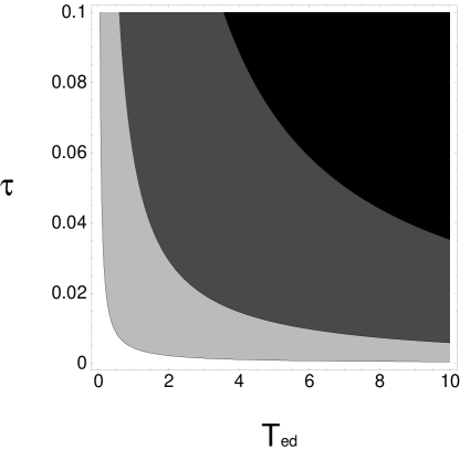
FIG. 1.: Contour plot of the quantity ${\cal R}$ as function of $\tau$ and $T_{ed}$. The values of other parameters are $\gamma=10^{-5}$, $T=10^{4}$ (frequencies and times are dimensionless since they are properly scaled through the system frequency). Contours values are $3$, $2$ and $1$, moving from bright to dark region.

IV Repeated correction procedure

The number of correction procedures applied during the time $T$ can be varied. Consider the problem of optimizing error correction to achieve the greatest probability success for the storage of a qubit state, given the freedom to apply an arbitrary number $N$ of encoding+decoding procedures during $T$. Assume that these are spaced out equally. In case of perfect error correction, it is obviously beneficial to apply as many corrections as possible. The probability of success for $N$ applications is

$${\cal P}_{N}=[{\cal P}_{s}^{*}(T/N)]^{N}\,.$$ (19)

This maximizes for $N\to\infty$, tending to unity. Such behavior is like the Zeno or watchdog effect; there is no change at all from the initial state as $N\to\infty$ [10].

However, in case of timing errors, there should be an optimum value of $N$. The generalization of Eq. (17) to $N$ equally spaced corrections is

$$P_{N}=[{\cal P}_{t}(T_{ed})]^{5N}\times[{\cal P}_{s}^{*}(T/N)]^{N}\,.$$ (20)

Then, in Figure 2 we plot $P_{N}$ as function of $N$. We see that the optimum number $N$ which maximize the probability decreases by increasing the value of $\tau$. In figure, we pass from $N_{opt}=6$ for $\tau=0.003$, to $N_{opt}=3$ for $\tau=0.01$, and $N_{opt}=1$ for $\tau=0.05$. Beyond that value the error correction becomes useless.

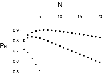
FIG. 2.: Success probability $P_{N}$ for $N$-repeated correction procedures as function of $N$, for different values of $\tau$ (circles $\tau=0.003$; squares $\tau=0.01$; triangles $\tau=0.05$). The values of other parameters in frequency units are $\gamma=10^{-5}$, $T=10^{4}$, $T_{ed}=1$ (frequencies and times are dimensionless since they are properly scaled trough the system frequency).

V Conclusion

In conclusion we have considered the problem of temporal imperfections in building up correcting codes. To this end we have exploited a quite ductile model based on random time evolution.

In Ref. [11] non-dissipative decoherence bounds for ion-trap based quantum computation were established by estimating $\tau\approx 10^{-3}$. In such a case $\tau$ gives an estimate of the pulse are fluctuations for the laser inducing transitions. This value of $\tau$ gives the restriction $T_{ed}/T<10^{-3}$ for the success of the above considered code.

Finally, we recognize that our approach is somewhat rough since the reversible dynamics during encoding and decoding has been identified with the free dynamics. Nevertheless, it allows an estimation of realistic performances of simple challenging codes. A more accurate study is left for future work.

REFERENCES

- [1] Nielsen, M. A., and Chuang, I. L., 2000, Quantum Computation and Quantum Information, (Cambridge University Press).
- [2] Shor, P. W., 1990, Phys. Rev. A, 52, 2493.
- [3] Steane, A. M., 1996, Phys. Rev. Lett., 77, 793.
- [4] Bennet, C. H., DiVincenzo, D. P., Smolin, J. A., and Wootters, W. K., 1996 Phys. Rev. A, 54, 3824; Laflamme, R., Miquel, C., Paz, J. P., and Zurek, W. H., 1996, Phys. Rev. Lett., 77, 198.
- [5] DiVincenzo, D. P., and Shor, P., 1996, Phys. Rev. Lett., 77, 3260; Steane, A. M., 1997, Phys. Rev. Lett., 78, 2252; Gottesman, D., 1998, Phys. Rev. A, 57, 127.
- [6] Chuang, I. L., and Yamamoto, Y., 1997, Phys. Rev. A, 55, 114; Barenco, A., Brun, T. A., Schack, R., and Spiller, T. P., 1997, Phys. Rev. A, 56, 1177.
- [7] Wineland, D. J., Monroe, C., Itano, W. M., Leibfried, D., King, B. E., and Meekhof, D. M., 1998, J. Res. NIST, 103, 259.
- [8] Jones, J. A., Hansen, R. H., and Mosca, M., 1998, J. Magn. Reson., 135, 353.
- [9] Bonifacio, R., 1999, Il Nuovo Cimento, 114 B, 473; Bonifacio, R., 1999 in Mysteries, Puzzles and Paradoxes in Quantum Mechanics, Ed. by Bonifacio, R. (AIP, Woodbury).
- [10] Misra, B., and Sudarshan, E. C. G., 1997, J. Math. Phys., 18, 756; Zurek, W. H., 1984, Phys. Rev. Lett., 53, 391.
- [11] Mancini, S., and Bonifacio, R., 2001, Phys. Rev. A, 63, 032310.