A security proof of quantum cryptography based entirely on entanglement purification

Abstract

We give a proof that entanglement purification, even with noisy apparatus, is sufficient to disentangle an eavesdropper (Eve) from the communication channel. In the security regime, the purification process factorises the overall initial state into a tensor-product state of Alice and Bob, on one side, and Eve on the other side, thus establishing a completely private, albeit noisy, quantum communication channel between Alice and Bob. The security regime is found to coincide for all practical purposes with the purification regime of a two-way recurrence protocol. This makes two-way entanglement purification protocols, which constitute an important element in the quantum repeater, an efficient tool for secure long-distance quantum cryptography.

I Introduction

A central problem of quantum communication is how to faithfully transmit unknown quantum states through a noisy quantum channel Schumacher (1996). While information is sent through such a channel (for example an optical fiber), the carriers of the information interact with the channel, which gives rise to the phenomenon of decoherence and absorption; an initially pure quantum state becomes a mixed state when it leaves the channel. For quantum communication purposes, it is necessary that the transmitted qubits retain their genuine quantum properties, for example in form of an entanglement with qubits on the other side of the channel.

In quantum cryptography Bennett and Brassard (1985); Ekert (1991), noise in the communication channel plays a crucial role: In the worst-case scenario, all noise in the channel is attributed to an eavesdropper, who manipulates the qubits in order to gain as much information on their state as possible, while introducing only a moderate level of noise Ekert et al. (1994); Fuchs and Peres (1996); Lütkenhaus (1996); Fuchs et al. (1997).

There are two well-established methods to deal with the problem of noisy channels. The theory of quantum error correction Calderbank and Shor (1996); Steane (1996) has mainly been developed to make quantum computation possible despite the effects of decoherence and imperfect apparatus. Since data transmission – like data storage – can be regarded as a special case of a computational process, clearly quantum error correction can also be used for quantum communication through noisy channels. An alternative approach, which has been developed roughly in parallel with the theory of quantum error correction, is the purification of mixed entangled states Bennett et al. (1996a, b); Deutsch et al. (1996).

In quantum cryptography, noise in the communication channel plays a crucial role: In the worst-case scenario, all noise in the channel is attributed to an eavesdropper, who manipulates the qubits in order to gain as much information on their state as possible, while introducing only a moderate level of noise.

To deal with this situation, two different techniques have been developed: Classical privacy amplification allows the eavesdropper to have partial knowledge about the raw key built up between the communicating parties Alice and Bob. From the raw key, a shorter key is “distilled” about which Eve has vanishing (i. e. exponentially small in some chosen security parameter) knowledge. Despite of the simple idea, proofs taking into account all eavesdropping attacks allowed by the laws of quantum mechanics have shown to be technically involved Mayers (1996); Biham et al. (2000); Inamori . Recently, Shor and Preskill Shor and Preskill (2000) have given a simpler physical proof relating the ideas in Mayers (1996); Biham et al. (2000) to quantum error correcting codes Calderbank and Shor (1996) and, equivalently, to one-way entanglement purification protocols Bennett et al. (1996b). Quantum privacy amplification (QPA) Deutsch et al. (1996), on the other hand, employs a two-way entanglement purification recurrence protocol that eliminates any entanglement with an eavesdropper by creating a few perfect EPR pairs out of many imperfect (or impure) EPR pairs. The perfect EPR pairs can then be used for secure key distribution in entanglement-based quantum cryptography Deutsch et al. (1996); Ekert (1991); Bennett et al. (1992). In principle, this method guarantees security against any eavesdropping attack. However, the problem is that the QPA protocol assumes ideal quantum operations. In reality, these operations are themselves subject to noise. As shown in Briegel et al. (1998); Dür et al. (1999); Giedke et al. (1999), there is an upper bound $F_{\text{max}}$ for the achievable fidelity of EPR pairs which can be distilled using noisy apparatus. A priori, there is no way to be sure that there is no residual entanglement with an eavesdropper. This problem could be solved if Alice and Bob had fault tolerant quantum computers at their disposal, which could then be used to reduce the noise of the apparatus to any desired level. This was an essential assumption in the security proof given by Lo and Chau Lo and Chau (1999).

In this paper, we show that the standard two-way entanglement purification protocol alone, with some minor modifications to accomodate certain security aspects as discussed below, can be used to efficiently establish a perfectly private quantum channel, even when both the physical channel connecting the parties and the local apparatus used by Alice and Bob are noisy.

In Section II we will briefly review the concepts of entanglement purification and of the quantum repeater, and discuss why it is interesting to combine the security features of entanglement purification with the long-distance feature of the quantum repeater. Section III will give the main result of our work: we prove that it is possible to factor out an eavesdropper using EPP, even when the apparatus used by Alice and Bob is noisy. One important detail in the proof is the flag update function, which we will derive in Section IV. We conclude the paper with a discussion in Section V.

II Entanglement purification and the quantum repeater

II.1 Entanglement purification

As two-way entanglement purification protocols (2–EPP) play an important role in this paper, we will briefly review one example of a a recurrence protocol which was described in Deutsch et al. (1996), and called quantum privacy amplification (QPA) by the authors. It is important to note that we distinguish the entanglement purification protocol from the distillation process: the first consists of probabilistic local operations (unitary rotations and measurements), where two pairs of qubits are combined, and either one or zero pairs are kept, depending on the measurement outcomes. The latter, on the other hand, is the procedure where the purification protocol is applied to large ensemble of pairs recursively (see Fig. (1)).

Figure 1: The entanglement purification protocol (a) and the entanglement distillation process (b).

In the quantum privacy amplification 2–EPP, two pairs of qubits, shared by Alice and Bob, are considered to be in the state $\rho_{A_{1}B_{1}}\otimes\rho_{A_{2}B_{2}}$. Without loss of generality (see later), we may assume that the state of the pairs is of the Bell-diagonal form,

$$\rho_{AB}=A\left|\Phi^{+}\right\rangle\!\left\langle\Phi^{+}\right|+B\left|\Psi^{-}\right\rangle\!\left\langle\Psi^{-}\right|+C\left|\Psi^{+}\right\rangle\!\left\langle\Psi^{+}\right|+D\left|\Phi^{-}\right\rangle\!\left\langle\Phi^{-}\right|.$$ (1)

Following Deutsch et al. (1996), the protocol consists of three steps:

1. Alice applies to her qubits a $\pi/2$ rotation, $U_{x}$, Bob a $-\pi/2$ rotation about the $x$ axis, $U_{x}^{-1}$.

2. Alice and Bob perform the bi-lateral CNOT operation

   $$\mathrm{BCNOT_{A_{1}B_{1}}^{A_{2}B_{2}}}=\mathrm{CNOT}_{A_{1}}^{A_{2}}\otimes\mathrm{CNOT}_{B_{1}}^{B_{2}}$$

   on the four qubits.

3. Alice and Bob measure both qubits of the target pair $A_{2}B_{2}$ of the BCNOT operation in the $z$ direction. If the measurement results coincide, the source pair $A_{1}B_{1}$ is kept, otherwise it is discarded. The target pair is always discarded, as it is projected onto a product state by the bilateral measurement.

By a straigtforward calculation, one gets the result that the state of the remaining pair is still a Bell diagonal state, with the diagonal coefficients Deutsch et al. (1996)

$$\begin{split}A^{\prime}&=\frac{A^{2}+B^{2}}{N},\quad B^{\prime}=\frac{2CD}{N}\\ C^{\prime}&=\frac{C^{2}+D^{2}}{N},\quad D^{\prime}=\frac{2AB}{N},\\ \end{split}$$ (2)

and the normalization coefficient $N=(A+B)^{2}+(C+D)^{2}$, which is the probability that Alice’s and Bob’s measurement results in step 3 coincide. Note that, up to the normalization, these recurrence relations are a quadratic form in the coefficients $A,B,C,$ and $D$. These relations allow for the following interpretation (which can be used to obtain the relations (2) in the first place): As all pairs are in the Bell diagonal state (1), one can interpret $A,B,C,$ and $D$ as the relative frequencies with which the states $\left|\Phi^{+}\right\rangle,\left|\Psi^{-}\right\rangle,\left|\Psi^{+}\right\rangle,$ and $\left|\Phi^{-}\right\rangle$, respectively, appear in the ensemble. By looking at (2) one finds that the result of combining two $\left|\Phi^{+}\right\rangle$ or two $\left|\Psi^{-}\right\rangle$ pairs is a $\left|\Phi^{+}\right\rangle$ pair, combining a $\left|\Psi^{+}\right\rangle$ and a $\left|\Phi^{-}\right\rangle$ (or vice versa) yields a $\left|\Psi^{-}\right\rangle$ pair, and so on. Combinations of $A,B,C,$ and $D$ that do not occur in (2), namely $AC$, $AD$, $BC$ and $BD$, are “filtered out”, i. e. they give different measurement results for the bilateral measurement in step 3 of the protocol. We will use this way of calculating recurrence relations for more complicated situations later.

Numerical calculations Deutsch et al. (1996) and, later, an analytical investigation Macchiavello (1998) have shown that for all initial states (1) with $A>1/2$, the recurrence relations (2) approach the fixpoint $A=1,B=C=D=0$; this means that given a sufficiently large number of initial pairs, Alice and Bob can distill asymptotically pure EPR pairs.

II.2 Entanglement purification with noisy apparatus and the quantum repeater

Under realistic conditions, the local operations (quantum gates, measurements) themselves, that constitute a purification protocol, will never be perfect and thus introduce a certain amount of noise to the ensemble when they are applied by Alice and Bob. The follow questions then arise: How does a protocol perform under the influence of local noise? How robust is it and what is the threshold for purification? These questions have been dealt with in Refs. Briegel et al. (1998); Dür et al. (1999); Giedke et al. (1999). The main results are, in brief, that for a finite level of local noise, there is a maximum achievable fidelity $F_{\text{max}}<1$ beyond which purification is not possible. Similarly, the minimum required fidelity $F_{\text{min}}>1/2$ for purification has increased with respect to the ideal protocol Bennett et al. (1996a). The purification regime $[F_{\text{min}},F_{\text{max}}]\in[1/2,1]$ has thus become smaller compared to the noiseless case. With an increasing noise level, the size of the purification regime shrinks until, at the purification threshold, $F_{\text{min}}$ and $F_{\text{max}}$ coincide and the protocol breaks down. At this point, the noise of the local operations corresponds to a loss of information that is larger than the gain of information ontained by a destillation step in the ideal case.

For a moderate noise level (of the order of a few percent for the recurrence protocols of Refs. Bennett et al. (1996a); Deutsch et al. (1996)), entanglement purification remains an efficient tool for establishing high-fidelity (although not perfect) EPR pairs, and thus for quantum communication over distances of the order of coherence length of a noisy channel. The restriction to the coherence length is due to the fact that the fidelity of the initial ensemble needs to be above the value $F_{\text{min}}(>1/2)$.

Long-distance quantum communication describes a situation where the length of the channel connecting the parties is typically much longer than its coherence- and absorption length. As the depolarisation errors and the absorption losses scale exponentially with the length of the channel, one cannot send qubits directly through the channel.

To solve this problem, there are two solutions known. The first is to treat quantum communication as a (very simplistic) special case of quantum computation. The methods of fault tolerant quantum computation Preskill (1998); Knill et al. (1996) and quantum error correction could then be used for the communication task. An explicit scheme for data transmission and storage has been discussed by Knill and Laflamme Knill and Laflamme (1996), using the method of concatenated quantum coding. While this idea shows that it is in principle possible to get polynomial or even polylogarithmic Kitaev (1997); Aharonov and Ben-Or ; Knill et al. (1998) scaling in quantum communication, it has an important drawback: long-distance quantum communication using this idea is as difficult as fault tolerant quantum computation, despite the fact that short distance QC is (from a technological point of view) already ready for practical use.

The other solution for the long-distance problem is the entanglement based quantum repeater (QR) Briegel et al. (1998); Dür et al. (1999) with two-way classical communication. It employs both entanglement purification Bennett et al. (1996a, b); Deutsch et al. (1996) and entanglement swapping Bennett et al. (1993); Zukowski et al. (1993); Pan et al. (1998) in a meta-protocol, the nested two-way entanglement purification protocol (NEPP). The apparatus used for quantum operations in the NEPP tolerates noise on the (sub-) percent level. As this tolerance is two orders of magnitude less restrictive than for fault tolerant quantum computation, it seems to make the quantum repeater a promising concept also for practical realisation in the future. Please note that the quantum repeater has been designed not only to solve the problem of decoherence, but also of absorption. For the latter, the possiblity of quantum storage is required at the repeater stations. An explicit implementation that takes into account absorption is given by the photonic channel of Ref. van Enk et al. (1997, 1998) (see also Briegel et al. (2000)).

II.3 The quantum repeater and quantum privacy amplification

The aim of this paper, as mentioned in the introduction, is to show that entanglement distillation using realistic apparatus is sufficient to create private entanglement between Alice and Bob, i. e. pairs of entangled qubits of which Eve is guaranteed to be disentangled even though they are not pure EPR pairs. If these pairs are used to teleport quantum information from Alice to Bob, they can be regarded as a noisy but private quantum channel.

This will also prove the security of quantum communication using the entanglement-based quantum repeater, since it is only necessary to consider the outermost entanglement purification step in the NEPP, which is performed by Alice and Bob exclusively, i.e. without the support of the parties at the intermediate repeater stations. In particular, it is not necessary to analyze the effect of noisy Bell measurements on the security. In the worst case scenario, Alice and Bob assume that all repeater stations are completely under Eve’s control, anyway. For this reason, Alice and Bob are not allowed to make assumptions on the method how the pairs have been distributed.

The role of the quantum repeater in the security proof is thus the following. It tells us that it is possible to distribute EPR pairs of high fidelity over arbitrary distances (with polynomial overhead), given that the noise level of the apparatus (or operations) used in the entanglement purification is below a certain (sub percent) level. The noise in the apparatus will reflect itself in the fact that the final distributed pairs between Alice and Bob are also imperfect (i.e. not pure Bell states), and so the question arises whether these imperfect pairs can be used for e.g. secure key distribution. The answer is yes. Since the security regime practically coincides with the purification regime (see Sec. III.4), quantum communication is guaranteed to be secure whenever the noise level of the local operations is in the operation regime of the quantum repeater.

III Factorization of Eve

In this section we will show that 2–EPP with noisy apparatus is sufficient to factor out Eve in the Hilbertspace of Alice, Bob, their laboratories, and Eve. For the proof, we will first introduce the concept of the lab demon as a simple model of noise. Then we will consider the special case of binary pairs, where we have obtained analytical results. Using the same techniques, we generalize the result to the case of Bell-diagonal ensembles. To conclude the proof, we show how the most general case of ensembles, described by an arbitray entangled state of all the qubits on Alice’s and Bob’s side, can be reduced to the case of Bell-diagonal ensembles.

III.1 The effect of noise

In this section we will answer the following question: what is the effect of an error, introduced by some noisy operation at a given point of the distillation process? We restrict our attention to the following type of noise:

• It acts locally, i. e. the noise does not introduce correlations between remote quantum systems.

• It is memoryless, i. e. on a timescale imposed by the sequence of steps in a given protocol, there are no correlations between the “errors” that occur at different times.

The action of noisy apparatus on a quantum system in state $\rho\in\mathcal{B}(\mathcal{H})$ can be formally described by some trace conserving, completely positive map. Any such map can be written in the operator-sum representation Kraus (1983); Schumacher (1996),

$$\rho\rightarrow\sum_{i}A_{i}\rho A_{i}^{\dagger},$$ (3)

with linear operators $A_{i}$, that fulfill the normalization condition $\sum_{i}AA^{\dagger}=\mathbf{1}$. The operators $A_{i}$ are the so-called Kraus operators Kraus (1983).

As we have seen above, in the purification protocol the CNOT operation, which acts on two qubits $a$ and $b$, plays an important role. For that reason, it is necessary to consider noise which acts on a two-qubit Hilbert space $\mathcal{H}=\mathbb{C}^{2}_{a}\otimes\mathbb{C}^{2}_{b}$. Eq. (3) describes the most general non-selective operation that can, in principle, be implemented. For technical reasons, however, we restrict our attention to the case that the Kraus operators are proportional to products of Pauli matrices. The reason for this choice is that Pauli operators map Bell states onto Bell states, which will allow us to introduce the very useful concept of error flags later. Eq. (3) can then be written as

$$\rho_{ab}\rightarrow\sum_{\mu,\nu=0}^{3}f_{\mu\nu}\sigma_{\mu}^{(a)}\sigma_{\nu}^{(b)}\rho_{ab}\sigma_{\mu}^{(a)}\sigma_{\nu}^{(b)}\,,$$ (4)

with the normalization condition $\sum_{\mu,\nu=0}^{3}f_{\mu\nu}=1$. Note that Eq. (4) includes, for an appropriate choice of the coefficients $f_{\mu\nu}$, the one- and two-qubit depolarizing channel and combinations thereof, as studied in Briegel et al. (1998); Dür et al. (1999); but it is more general. Below, we will refer to these special Kraus operators as error operators.

The proof can be extended to more general noise models if a slightly modified protocol is used, where the twirl operation of step 1 is repeated after every distillation round . The concatenated operation, which consists of a general noisy operation followed by this regularization operation, is Bell diagonal i. e. it maps Bell-diagonal states onto Bell-diagonal states, but since it maps all states to a Bell-diagonal state, it clearly cannot be written in the form (4). However, for the purpose of the proof, it is in fact only necessary that the concatenated map restricted to the space of all Bell-diagonal ensembles can be written in the form (4); we call such a map a restricted Bell-diagonal map. Clearly, not all restricted Bell-diagonal maps are of the form (4), which can be seen considering a map which maps any Bell diagonal state to a pure Bell state. Such a map could, however, not be implemented locally. Thus the question remains whether a restricted Bell-diagonal map which can be implemented locally can be written in the form (4). Though we are not aware of a formal proof of such a theorem, we conjecture that it holds true: the reduced density operator of each qubit must remain in the maximally mixed state, which is indeed guaranteed by a mixture of unitary rotations. We also have numerical evidence which supports this conjecture. Note that in the case of such an active regularization procedure, it is important that the Pauli rotations in step 1 can be performend well enough to keep the evolution Bell diagonal. This is, however, not a problem, since Alice and Bob are able to propagate the Pauli rotations through the unitary operations of the EPP, which allows them to perform the rotations just before a measurement, or, equivalently, to rotate the measurement basis. This is similar to the concept of error correctors (where the error consists in ommiting a required Pauli operaton), as described in Section IV.1, and to the by-product matrix formalism developed in Raussendorf and Briegel (2001).

The coefficients $f_{\mu\nu}$ in (4) can be interpreted as the joint probability that the Pauli rotations $\sigma_{\mu}$ and $\sigma_{\nu}$ occur on qubits $a$ and $b$, respectively. For pedagogic purposes we employ the following interpretation of (4): Imagine that there is a (ficticious) little demon in Alice’s laboratory – the “lab demon” – which applies in each step of the distillation process randomly, according to the probability distribution $f_{\mu\nu}$, the Pauli rotation $\sigma_{\mu}$ and $\sigma_{\nu}$ to the qubits $a$ and $b$, respectively. The lab demon summarizes all relevant aspects of the lab degrees of freedom involved in the noise process.

Noise in Bob’s laboratory, can, as long as we restrict ourselves to Bell diagonal ensembles, be attributed to noise introduced by Alice’s lab demon, without loss of generality; this is, however, not a crucial restriction, as we will show in Section III.5. It is also possible to think of a second lab demon in Bob’s lab who acts similarly to Alice’s lab demon. This would, however, not affect the arguments employed in this paper.

The lab demon does not only apply rotations randomly, he also maintains a list in which he keeps track of which rotation he has applied to which qubit pair in which step of the distillation process. What we will show in the following section is that, from the mere content of this list, the lab demon will be able to extract – in the asymptotic limit – full information about the state of each residual pair of the ensemble. This will then imply that, given the lab demons knowledge, the state of the distilled ensemble is a tensor product of pure Bell states. Furthermore, Eve cannot have information on the specific sequence of Bell pairs (beyond their relative frequencies) — otherwise she would also be able to learn, to some extent, at which stage the lab demon has applied which rotation.

From that it follows that Eve is factored out, i. e. the overall state of Alice’s, Bob’s and Eve’s particles is described a density operator of the form

$$\rho_{\mathrm{ABE}}=\left(\sum_{i,j=0}^{1}f^{(i,j)}\left|\mathcal{B}_{i,j}\right\rangle_{\!\mathrm{AB}}\!\left\langle\mathcal{B}_{i,j}\right|\right)\otimes\rho_{\mathrm{E}}\,,$$ (5)

where $\sum_{i,j}f^{(i,j)}=1$, and $\mathcal{B}_{i,j}$ describe the four Bell states as defined in Sec. III.5.

Note that the lab demon was only introduced for pedagogical reasons. In reality, there will be other mechanisms of noise. However, all physical processes that result in the same completely positive map (4) are equivalent, i. e. cannot be distinguished from each other if we only know how they map an input state $\rho_{i}$ onto an output state $\rho_{f}$. In particular, the processes must lead to the same level of security (regardless whether or not error flags are measured or calculated by anybody): otherwise they would be distinguishable.

In order to separate conceptual from technical considerations and to obtain analytical results, we will first concentrate on the special case of binary pairs and a simplified error model. After that, we generalize the results to any initial state.

III.2 Binary pairs

In this section we restrict our attention to pairs in the state

$$\rho_{AB}=A\left|\Phi^{+}\right\rangle_{\!AB}\!\left\langle\Phi^{+}\right|+B\left|\Psi^{-}\right\rangle_{\!AB}\!\left\langle\Psi^{-}\right|,$$ (6)

and to errors of the form

$$\rho_{AB}^{(1)}\otimes\rho_{AB}^{(2)}\rightarrow\sum_{\mu,\nu\in\{0,1\}}f_{\mu\nu}U^{(1)}_{\mu}U^{(2)}_{\nu}\rho_{AB}^{(1)}\otimes\rho_{AB}^{(2)}{U^{(1)}_{\mu}}^{\dagger}{U^{(2)}_{\nu}}^{\dagger}$$ (7)

with $U_{0}^{(1,2)}=\text{id}^{(1,2)}$ and $U_{1}^{(1,2)}={\sigma_{x}}^{(1,2)}$. Eq. (7) describes a two-bit correlated spin-flip channel. The indices 1 and 2 indicate the source and target bit of the bilateral CNOT (BCNOT) operation, respectively. It is straightforward to show that, using this error model in the 2–EPP, binary pairs will be mapped onto binary pairs.

At the beginning of the distillation process, Alice and Bob share an ensemble of pairs described by (6). Let us imagine that the lab demon attaches one classical bit to each pair, which he will use for book-keeping purposes. At this stage, all of these bits, which we call “error flags”, are set to zero. This reflects the fact that the lab demon has the same a priori knowledge about the state of the ensemble as Alice and Bob.

In each purification step, two of the pairs are combined. The lab demon first simulates the noise channel (7) on each pair of pairs by the process described. Whenever he applies a $\sigma_{x}$ operation to a qubit, he inverts the error flag of the corresponding pair. Alice and Bob then apply the 2–EPP to each pair of pairs; if the measurement results in the last step of the protocol coincide, the source pair will be kept. Obviously, the error flag of that remaining pair will also depend on the error flag of the the target pair, i. e. the error flag of the remaining pair is a function of the error flags of both “parent” pairs, which we call the flag update function. In the case of binary pairs, the flag update function maps two bits (the error flags of both parents) onto one bit. In total, there exist 16 different functions $f\!:\!\{0,1\}^{2}\to\{0,1\}$. From these, the lab demon chooses the logical AND function as the flag update function, i. e. the error flag of the remaining pair is set to “1” if and only if both parent’s error flags had the value “1”.

After each purification step, the lab demon divides all pairs into two subensembles, according to the value of their error flags. By a straightforward calculation, we obtain for the coefficients $A_{i}$ and $B_{i}$, which completely describe the state of the pairs in the subensemble with error flag $i$, the following recurrence relations:

$$\begin{split}A_{0}^{\prime}=&\frac{1}{N}(f_{00}(A_{0}^{2}+2A_{0}A_{1})+f_{11}(B_{1}^{2}+2B_{0}B_{1})\\ &+f_{s}(A_{0}B_{1}+A_{1}B_{1}+A_{0}B_{0}))\\ A_{1}^{\prime}=&\frac{1}{N}\left(f_{00}A_{1}^{2}+f_{11}B_{0}^{2}+f_{s}A_{1}B_{0}\right)\\ B_{0}^{\prime}=&\frac{1}{N}(f_{00}(B_{0}^{2}+2B_{0}B_{1})+f_{11}(A_{1}^{2}+2A_{0}A_{1})\\ &+f_{s}(B_{0}A_{1}+B_{1}A_{1}+B_{0}A_{0}))\\ B_{1}^{\prime}=&\frac{1}{N}\left(f_{00}B_{1}^{2}+f_{11}A_{0}^{2}+f_{s}B_{1}A_{0}\right)\end{split}$$ (8)

with $N=(f_{00}+f_{11})((A_{0}+A_{1})^{2}+(B_{0}+B_{1})^{2})+2f_{s}(A_{0}+A_{1})(B_{0}+B_{1})$ and $f_{s}=f_{01}+f_{10}$.

For the case of uncorrelated noise, $f_{\mu\nu}=f_{\mu}f_{\nu}$, we obtain the following analytical expression for the relevant fixpoint of the map (8):

$$\begin{split}A_{0}^{\infty}&=\frac{4f_{0}^{2}-4f_{0}+(2f_{0}-1)\sqrt{4f_{0}-3}+1}{2(2f_{0}-1)^{2}},\\ A_{1}^{\infty}&=0,\quad B_{0}^{\infty}=0,\quad B_{1}^{\infty}=1-A_{0}^{\infty}.\end{split}$$ (9)

Note that, while Eq. (9) gives a fixpoint of (8) for $f_{0}\geq 3/4$, this does not imply that this fixpoint is an attractor. In order to investigate the attractor properties, we calculate the eigenvalues of the matrix of first derivatives,

$$M_{D}=\left.\left(\begin{array}[]{c c c}\frac{\partial A_{0}^{\prime}}{\partial A_{0}}&\cdots&\frac{\partial B_{1}^{\prime}}{\partial A_{0}}\\ \vdots&\ddots&\vdots\\ \frac{\partial A_{0}^{\prime}}{\partial B_{1}}&\cdots&\frac{\partial B_{1}^{\prime}}{\partial B_{1}}\\ \end{array}\right)\right|_{\mathrm{fixpoint}}\quad.$$ (10)

We find that the modulus of the eigenvalues of this matrix is smaller than unity for $f_{0}^{\mathrm{crit}}=0.77184451<f_{0}\leq 1$, which means that in this interval, the fixpoint (9) is also an attractor. This is in excellent agreement with a numerical evaluation of (8), where we found that $0.77182<f_{0}^{\mathrm{crit}}<0.77188$.

We have also evaluated (8) numerically in order to investigate correlated noise (see Fig. 2). Like in the case of uncorrelated noise, we found that the coefficients $A_{0}$ and $B_{1}$ reach, during the distillation process, some finite value, while the coefficients $A_{1}$ and $B_{0}$ decrease exponentially fast, whenever the noise level is moderate.

In other words, both subensembles, characterized by the value of the respective error flags, approach a pure state asymptotically: The pairs in the ensemble with error flag “0” are in the state $\left|\Phi^{+}\right\rangle$, while those in the ensemble with error flag “1” are in the state $\left|\Psi^{+}\right\rangle$.

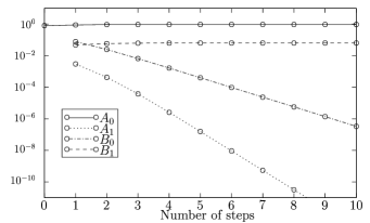
Figure 2: The evolution of the four parameters $A_{0},A_{1},B_{0}$, and $B_{1}$ in the security regime. Note that both $A_{1}$ and $B_{0}$ decrease exponentially fast in the number of steps. The initial fidelity was 80%, and the values of the noise parameters were $f_{00}=0.8575$, $f_{01}=f_{10}=f_{11}=0.0475$.

A map of the fixpoints

In Fig. 3, the values of $A_{0}^{\infty},A_{1}^{\infty},B_{0}^{\infty},B_{1}^{\infty},F^{\infty},$ and $F^{\mathrm{cond,\infty}}$ have been plotted as a function of the noise parameter $f_{0}$. Most interesting in this graph is the shape of the curve representing the conditional fidelity: For all noise parameters $f_{0}\leq 0.75$, the conditional fidelity reaches at the fixpoint the value $0.5$, while for noise parameters $f_{0}\geq 0.77184451$, the conditional fidelity reaches unity. In the intermediate regime ($0.75<f_{0}<77184451$), the curve can be fitted by a square root function $F^{\mathrm{cond}}(f_{0})=0.5+3.4\sqrt{f_{0}-0.75}.$

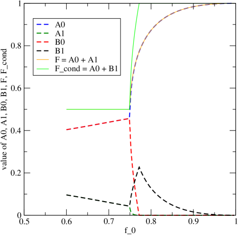
Figure 3: The values of $A_{0},A_{1},B_{0},B_{1},F,F^{\mathrm{cond}}$ at the fixpoint as a function of the noise parameter $f_{0}$.

The emergence of the intermediate regime of noise parameters, where the 2–EPP is able to purify and the lab demon does not gain full information on the state of the pairs is somewhat surprising and shows that the factorization of the eavesdropper is by no means a trivial consequence of (noisy) EPP. From a mathematical point of view, it is consistent with the finding after Eq. (10).

The purification curve

To understand the emergence of the intermediate regime better, we have plotted the purification curve for binary pairs, i. e. the $F^{\mathrm{cond}}_{n}-F^{\mathrm{cond}}_{n+1}$-diagram. A problem with this diagram is that the state of the pairs is specified by three independent parameters ($A_{0},A_{1},B_{0},B_{1}$ minus normalization), so that such plots can only show a specific section through the full parameter space. Below we explain in detail how these sections have been constructed. Fig. 4 shows an overdrawn illustration of what we found: for noise parameters close to the purification threshold, the purification curves have a point of inflection. If the noise level increases (i. e. $f_{0}$ decreases), the curves are quasi “pulled down”. For $f_{0}=0.77184451$, the slope of the purification curve at the fixpoint $F^{\mathrm{cond}}=1$ equals unity. If we further decrease $f_{0}$, the fixpoint is no longer an attractor, but due to the existence of the point of inflection, a new attractive fixpoint appeares.

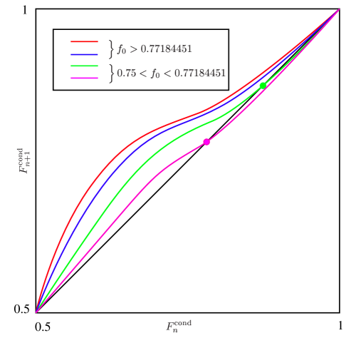
Figure 4: Illustration of the purification curve for variouse noise levels $f_{0}$. In order to make the point clear, the effect has been strongly overdrawn. See text.

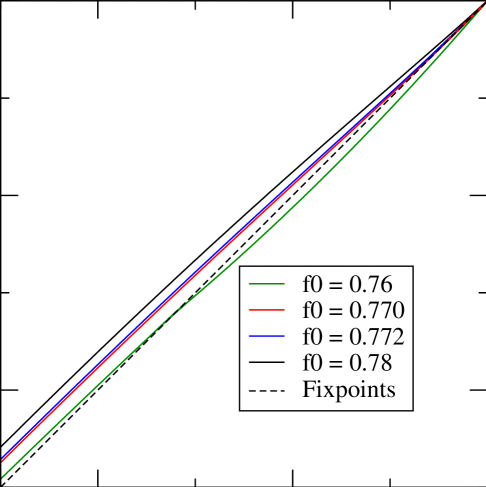
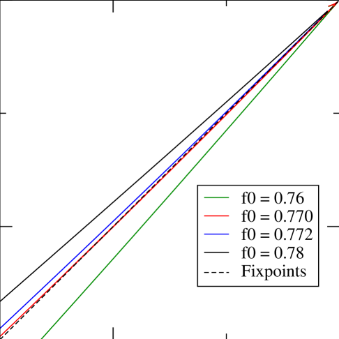
Figure 5: Actual data from which Fig. (4) has been infered.

To obtain the one-parametric curves shown in Fig 5, we used the following technique: starting with the point $(A_{0},A_{1},B_{0},B_{1})^{n=0}=(0.6,0,0.4,0)$, we calculated $(A_{0},A_{1},B_{0},B_{1})^{n=1}$ by applying the recursion relations (8) once. The points on the straight line in parameter space connecting these two points have then been used as input values for the map given by the $n$th power of (8). For the plot, the resulting curve segments have been concatenated. This procedure has been repeated for all noise parameters $f_{0}$ that are specified in Fig. 5. Note that at the critical value $f_{0}^{\mathrm{crit}}=0.77184451$, the number of iterations required to reach any $\epsilon$-environment of the fixpoint diverges. This fact will later be discussed in a more general case, see Fig. 9.

To conclude this section, we summarize: For all values $0.77184451\equiv f_{0}^{\mathrm{crit}}\leq f_{0}\leq 1$ the 2–EPP purifies and at the same time any eavesdropper is factored out. In a small interval, $0.75<f_{0}<f_{0}^{\mathrm{crit}}\equiv 0.77184451$, just above the threshold of the purification protocol, the conditional fidelity does not reach unity, while the protocol is in the purification regime. Even though this interval is small and of little practical relevance (for these values of $f_{0}$ we are already out of the repeater regime Briegel et al. (1998) and purification is very inefficient), its existence shows that the process of factorization is not trivially connected to the process of purification.

III.3 Bell-diagonal initial states

Now we want to show that the same result is true for arbitrary Bell diagonal states (Eq. (1)) and for noise of the form (4). The procedure is the same as in the case of binary pairs; however, a few modifications are required.

In order to keep track of the four different error operators $\sigma_{\mu}$ in (4), the lab demon has to attach two classical bits to each pair; let us call them the phase error bit and amplitude error bit. Whenever a $\sigma_{x}$ ($\sigma_{z}$, $\sigma_{y}$) error occurs, the lab demon inverts the error amplitude bit (error phase bit, both error bits). To update these error flags, he uses the update function given in Tab. 1. The physical reason for the choice of the flag update function will be given in the next section.

	(00)	(01)	(10)	(11)
(00)	(00)	(00)	(00)	(10)
(01)	(00)	(01)	(11)	(00)
(10)	(00)	(11)	(01)	(00)
(11)	(10)	(00)	(00)	(00)

Table 1: The value (phase error,amplitude error) of the updated error flag of a pair that is kept after a 2–EPP step, given as a function of the error flags of $P_{1}$ and $P_{2}$ (left to right and top to bottom, respectively).

Here, the lab demon divides all pairs into four subensembles, according to the value of their error flag. In each of the subensembles the pairs are described by a Bell diagonal density operator, like in Eq. (1), which now depends on the subensemble. That means, in order to completely specify the state of all four subensembles, there are 16 real numbers $A^{ij},B^{ij},C^{ij},D^{ij}$ with $i,j\in\{0,1\}$ required, for which one obtaines recurrence relations of the form

$$\begin{split}A^{(00)}_{n}&\rightarrow A^{(00)}_{n+1}(A^{(00)}_{n},A^{(01)}_{n},\ldots,D^{(11)}_{n}),\\ A^{(01)}_{n}&\rightarrow A^{(01)}_{n+1}(A^{(00)}_{n},A^{(01)}_{n},\ldots,D^{(11)}_{n}),\\ &\,\,\,\vdots\\ D^{(11)}_{n}&\rightarrow D^{(11)}_{n+1}(A^{(00)}_{n},A^{(01)}_{n},\ldots,D^{(11)}_{n}).\\ \end{split}$$ (11)

These generalize the recurrence relations (8) for the case of binary pairs, and the relations (2) for the case of noiseless apparatus.

Like the recurrence relations (2) and (8), respectively, these relations are (modulo normalization) quadratic forms in the 16 state variables $\vec{a}=\left(A^{(00)},A^{(00)},\ldots,D^{(11)}\right)^{T}$, with coefficients that depend on the error parameters $f_{\mu\nu}$ only. In other words, (11) can be written in the more compact form

$$\vec{a}^{\prime}_{j}=\vec{a}M_{j}\vec{a}^{T},$$ (12)

where, for each $j\in\{1,\ldots 16\}$, $M_{j}$ is a real $16\times 16$-matrix whose coefficients are polynomials in the noise parameters $f_{\mu\nu}$.

III.4 Numerical results

The 16 recurrence relations (11) imply a reduced set of 4 recurrence relations for the quantities $A_{n}=\sum_{ij}A_{n}^{(ij)}$, $\ldots$, $D_{n}=\sum_{ij}D_{n}^{(ij)}$ that describe the evolution of the total ensemble (that is, the blend Englert (1999) of the four subensembles) under the purification protocol. Note that these values are the only ones which are known and accessible to Alice and Bob, as they have no knowledge of the values of the error flags. It has been shown in Briegel et al. (1998) that under the action of the noisy entanglement distillation process, these quantities converge towards a fixpoint $(A_{\infty},B_{\infty},C_{\infty},D_{\infty})$, where $A_{\infty}=F_{\text{max}}$ is the maximal attainable fidelity Dür et al. (1999).

Fig. 6 shows for typical initial conditions the evolution of the 16 coefficients $A_{n}^{(00)}\ldots D_{n}^{(11)}$. They are organized in a $4\times 4$-matrix, where one direction represents the Bell state of the pair, and the other indicates the value of the error flag. The figure shows the state (a) at the beginning of the entanglement purification procedure, (b) after few purification steps, and (c) at the fixpoint. As one can see, initially all error flags are set to zero and the pairs are in a Werner state with a fidelity of $70\%$. After a few steps, the population of the diagonal elements starts to grow; however, none of the elements vanishes. At the fixpoint, all off-diagonal elements vanish, which means that there are strict correlations between the states of the pairs and their error flags.

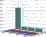
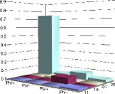
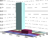
Figure 6: Typical evolution of the extended state under the purification protocol for the noise parameters $f_{00}=0.83981,f_{0j}=f_{i0}=0.021131$ and $f_{ij}=0.003712$ for $i,j\in\{1,2,3\}$. This corresponds to a combination of one- and two-qubit white noise, as studied in Briegel et al. (1998); Dür et al. (1999), with noise parameters $p_{1}=0.92$ and $p_{2}=0.9466$, considering noise in Alice’s lab only, or $p_{1}=0.9592$ and $p_{2}=0.973$, considering noise in Alice’s and Bob’s laboratory. We have choosen these values for didactical reasons, in order to make the effect more visible.

In order to determine how fast the state converges, we investigate two important quantities: the first is the fidelity $F_{n}\equiv A_{n}$, and the second is the conditional fidelity $F_{n}^{\text{cond}}\equiv A_{n}^{(00)}+B_{n}^{(11)}+C_{n}^{(01)}+D_{n}^{(10)}$. Note that the first quantity is the sum over the four $\left|\Phi^{+}\right\rangle$ components in Fig. 6, while the latter is the sum over the four diagonal elements. The conditional fidelity is the fidelity which Alice and Bob would assign to the pairs if they knew the values of the error flags, i. e.

$$F_{n}^{\text{cond}}=\sum_{i,j}\left\langle\Phi^{+}\right|\sigma_{i,j}\rho_{i,j}\sigma_{i,j}\left|\Phi^{+}\right\rangle,$$ (13)

where $\rho_{i,j}$ is the non-normalized state of the subensemble of the pairs with the error flag $(i,j)$. For convenience, we use the phase- and spin-flip bits $i$ and $j$ as indices for the Pauli matrices, i. e. $\sigma_{00}=\mathrm{Id},\sigma_{01}=\sigma_{x},\sigma_{11}=\sigma_{y},\sigma_{10}=\sigma_{z}$. We will utilize the advantages of this notation in Section IV.

Figure 7: The fidelities $F$ and $F_{\text{cond}}$ as a function of the number of steps in the security regime of the entanglement distillation process (analytical results (lines) and Monte Carlo simulation (circles)). The noise parameters for this plot were $f_{00}=0.91279120$, $f_{0j}=f_{i0}=0.0113896$ and $f_{ij}=0.0020968$ for $i,j\in\{1,2,3\}$, corresponding to white noise with noise parameters $p_{1}=0.96$ and $p_{2}=0.968$ (see Fig. 6). The Monte Carlo simulation was started with 10000000 pairs; the numbers indicate how many pairs are left after each step of the distillation process. This decreasing number is the reason for the increasing fluctuations around the analytical curves.

The results that we obtain are similar to those for the binary pairs. We can again distinguish three regimes of noise parameters $f_{\mu\nu}$. In the high-noise regime (i. e., small values of $f_{00}$), the noise level is above the threshold of the 2–EPP and both the fidelity $F$ and the conditional fidelity $F^{\mathrm{cond}}$ converge to the value 0.25. In the low-noise regime (i. e., large values of $f_{00}$), F converges to the maximum fidelity $F_{\mathrm{max}}$ and $F^{\mathrm{cond}}$ converges to unity (see Fig. 7). This regime is the security regime, where we know that secure quantum communication is possible. Like for binary pairs, there exists also an intermediate regime, where the 2–EPP purifies but $F^{\mathrm{cond}}$ does not converge to unity. For an illustration, see Fig 8. Note that the size of the intermediate regime is very small, compared to the security regime. Whether or not secure quantum communication is possible in this regime is unknown. However, the answer to this question is irrelevant for all practical purposes, because in the intermediate regime the distillation process converges very slowly, as shown in Fig. 9. In fact, the divergent behaviour of the process near the critical points has features remnant of a phase transition in statistical mechanics.

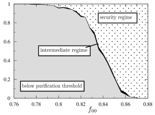
Figure 8: The size and the location of the three regimes of the distillation process. For fixed values of $f_{00}$, the remaining 15 noise parameters $f_{\mu\nu}$ have been choosen at random. Plotted is the relative frequency of finding the noise parameters in any of the three regimes as a function of $f_{00}$.

To estimate the size of the intermediate regime and to compare it to the case of binary pairs (Fig. 3), we consider the case of one-qubit white noise, i.e. $f_{\mu\nu}=f_{\mu}f_{\nu}$ and $f_{1}=f_{2}=f_{3}=(1-f_{0})/3$. Here, this regime is known to be bounded by

$$0.8983<f^{\mathrm{crit,lower}}<f_{0}<f^{\mathrm{crit,upper}}<0.8988.$$

Note that the size of the intermediate regime is much smaller than in the case of binary pairs.

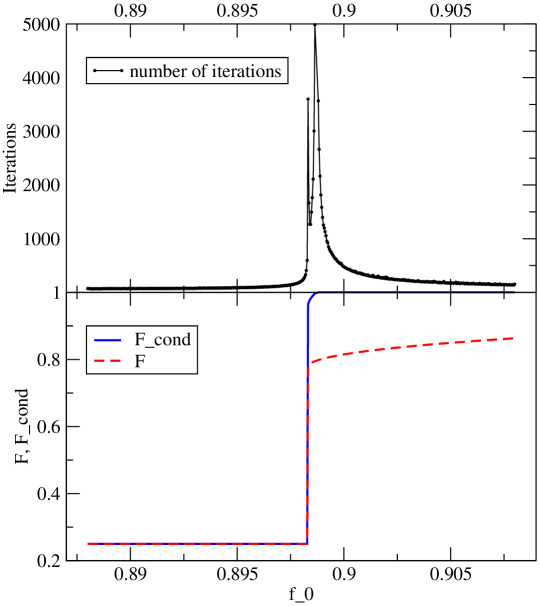
Figure 9: The effect of one-qubit white noise on the fidelity $F$, the conditional fidelity $F^{\text{cond}}$ and the number of iterations required for the convergence up to an uncertainty $\epsilon=10^{-12}$.

Regarding the efficiency of the distillation process, it is an important question how many initial pairs are needed to create one pair with fidelity $F^{\text{cond}}$, corresponding to the security parameter $\epsilon\equiv 1-F^{\text{cond}}$. Both the number of required initial pairs (resources) and the security parameter scale exponentially with the number of distillation steps, so that we expect a polynomial relation between the resources and the security parameter $\epsilon$. Fig. 10 confirms this relation in a log-log plot for different noise parameters. The straight lines are fitted polynomial relations; the fit region is indicated by the lines themselves.

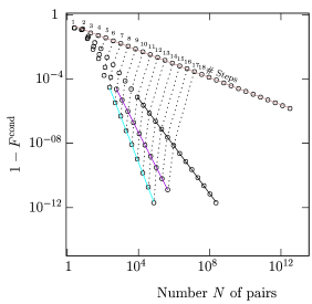
Figure 10: Number $N$ of pairs needed to create one pair with conditional fidelity $F^{\rm cond}$. The initial state of the pairs was of the Werner type with fidelity $F_{0}$ = 85%. One- and two-qubit white noise (see Fig. 6) has been assumed with the noise parameters $(p_{1},p_{2})=(0.9333,0.9466)$, $(0.9733,0.9786)$, $(0.9866,0.9833)$, $(0.9933,0.9946)$ (from top to bottom).

III.5 Non-Bell-diagonal pairs

In the worst-case scenario, Eve generates an ensemble of $N$ qubit pairs which she distributes to Alice and Bob. For that reason, Alice and Bob are not allowed to make specific assumptions on the state of the pairs. Most generally, the state of the $2N$ qubits, of which Alice and Bob obtain $N$ qubits each, can be written in the form

$$\rho_{AB}=\sum_{\mu_{1}\dots\mu_{N}\atop\mu_{1}^{\prime}\dots\mu_{N}^{\prime}}\alpha_{\mu_{1}\ldots\mu_{N}\atop\mu_{1}^{\prime}\ldots\mu_{N}^{\prime}}|{\cal B}_{\mu_{1}}^{(a_{1}b_{1})}\cdots{\cal B}_{\mu_{N}}^{(a_{N}b_{N})}\rangle\!\langle{\cal B}_{\mu_{1}^{\prime}}^{(a_{1}b_{1})}\cdots{\cal B}_{\mu_{N}^{\prime}}^{(a_{N}b_{N})}|.$$ (14)

Here, $|\mathcal{B}_{\mu_{j}}^{(a_{j}b_{j})}\rangle$, ${\mu_{j}}=00,01,10,11$ denote the 4 Bell states associated with the two particles $a_{j}$ and $b_{j}$ and $j=1,\ldots,N$. Specifically, $\left|\mathcal{B}_{00}\right\rangle\equiv\left|\Phi^{+}\right\rangle=\left(\left|00\right\rangle+\left|11\right\rangle\right)/\sqrt{2}$, $\left|\mathcal{B}_{01}\right\rangle\equiv\left|\Psi^{+}\right\rangle=\left(\left|01\right\rangle+\left|01\right\rangle\right)/\sqrt{2}$, $\left|\mathcal{B}_{10}\right\rangle\equiv\left|\Phi^{-}\right\rangle=\left(\left|00\right\rangle-\left|11\right\rangle\right)/\sqrt{2}$, $\left|\mathcal{B}_{11}\right\rangle\equiv\left|\Psi^{-}\right\rangle=\left(\left|01\right\rangle-\left|10\right\rangle\right)/\sqrt{2}$. In general, (14) will be an entangled state of $2N$ particles, which might moreover be entangled with additional quantum systems in Eve’s hands; this allows for the possibility of so-called coherent attacks Cirac and Gisin (1997).

Upon reception of all pairs, Alice and Bob apply the following protocol to them. Note that steps 1 and 2 are only applied once, while steps 3, 4, and 5 are applied recursively in the subsequent distillation process.
Step 1: On each pair of particles $(a_{j},b_{j})$, they apply randomly one of the four bi-lateral Pauli rotations $\sigma_{k}^{(a_{j})}\otimes\sigma_{k}^{(b_{j})}$, where k = 0,1,2,3.
Step 2: Alice and Bob randomly renumber the pairs, $(a_{j},b_{j})\to(a_{\pi(j)},b_{\pi(j)})$ where $\pi(j)$, $j=1,\dots,N$ is a random permutation.

Steps 1 and 2 are required in order to treat correlated pairs correctly. Note that steps 1 and 2 would also be required — as “preprocessing” steps — for the ideal distillation process Deutsch et al. (1996), if one requires that the process converges for arbitrary states of the form (14) to an ensemble of pure EPR states. While in Deutsch et al. (1996) it is possible to check whether or not the process converges to the desired pure state, by measuring the fidelity of some of the remaining pairs, this is not possible when imperfect apparatus is used. Since the maximum attainable fidelity $F_{\mathrm{max}}$ is smaller than unity, there is no known way to exclude the possibility that the non-ideal fidelity is due to correlations between the initial pairs. In both steps Alice and Bob discard the information which of the rotations and permutations, respectively, were chosen by their random number generator. Thus they deliberately loose some of the information about the ensemble which is still available to Eve (as she can eavesdrop the classical information that Alice and Bob exchange to implement step 1). After step 1, their knowledge about the state is summarized by the density operator

$$\tilde{\rho}_{AB}=\sum_{\mu_{1}\dots\mu_{N}}p_{\mu_{1}\dots\mu_{N}}|{\cal B}_{\mu_{1}}^{(a_{1}b_{1})}\cdots{\cal B}_{\mu_{N}}^{(a_{N}b_{N})}\rangle\langle{\cal B}_{\mu_{1}}^{(a_{1}b_{1})}\cdots{\cal B}_{\mu_{N}}^{(a_{N}b_{N})}|$$ (15)

which corresponds to a classically correlated ensemble of pure Bell states. Since the purification protocol that they are applying in the following steps maps Bell states onto Bell states, it is statistically consistent for Alice and Bob to assume after step 1 that they are dealing with a (numbered) ensemble of pure Bell states, where they have only limited knowledge about which Bell state a specific pair is in. The fact that the pairs are correlated means that the order in which they appear in the numbered ensemble may have some pattern, which may have been imposed by Eve or by the channel itself. By applying step 2, Alice and Bob $(i)$ deliberately ignore this pattern and $(ii)$ randomize the order in which the pairs are used in the subsequent purification steps . For all statistical predictions made by Alice and Bob, they may consistently describe the ensemble by the density operator

$$\tilde{\tilde{\rho}}_{AB} = \left(\sum_{\mu}p_{\mu}|{\cal B}_{\mu}\rangle\langle{\cal B}_{\mu}|\right)^{\otimes N}\equiv(\rho_{ab})^{\otimes N}$$ (16)

in which the $p_{\mu}$ describe the probability with which each pair is found in the Bell state $|{\cal B}_{\mu}\rangle$. At this point, Alice and Bob have to make sure that $p_{00}\equiv F>F_{\text{min}}$ for some minimum fidelity $F_{\text{min}}>1/2$, which depends on the noise level introduced by thier local apparatus. This test can be performed locally by statistical tests on a certain fraction of the pairs.

As Alice and Bob now own an ensemble of Bell diagonal pairs, they may proceed as described in the previous section. However, it is a reasonable question why Eve cannot take advantage of the additional information which she has about the state of the pairs: as she is allowed to keep the information about the twirl operations in step 1 and 2, from her point of view all the pairs remain in an highly entangled $2N$-qubit state. Nevertheless, all predicions made by Eve must be statistically consistent with the predictions made by Alice and Bob (or, for that matter, their lab demon), which means that the state calculated by Eve must be the same as the state calculated by the lab demon, tracing out Eve’s additional information. As the lab demon gets a pure state at the end of the entanglement distillation process, this must also be the result which Eve obtains using her additional information, simply due to the fact that no pure state can be written as a non-trivial convex combination of other states.

IV How to calculate the flag update function

In this section, we analyse how errors are propagated in the distillation process. As was mentioned earlier, the state of a given pair that survives a given purification step in the distillation process depends on all errors that occured on pairs in earlier steps, which belong to the “family tree” of this pair. Each step of the distillation process consist of a number of unitary operations followed by a measurement, which we want to treat separately.

IV.1 Unitary transformations and errors

Consider an error $U_{\text{err}}$ (i.e. a random unitary transformation) that is introduced before a unitary transformation $U$ is performed on a state $\left|\psi\right\rangle$. Note that, without loss of generality, it is always possible to split up a noisy quantum operation close to a unitary operation $U$ in two parts: first, a noisy operation close to identity, and afterwards the noiseless unitary operation $U$. For that reason, it only a matter of interpretation whether we think of a quantum operation which is accompanied by noise, e. g. as described by a master equation of the Lindblad form, or of the combination of some noise channel first and the noiseless quantum operation afterwards.

We call a transformation $U_{\text{corr}}$ an error corrector, if the equation

$$U\left|\psi\right\rangle=U_{\text{corr}}UU_{\text{err}}\left|\psi\right\rangle$$ (17)

holds for all states $\left|\psi\right\rangle$. Equation (17) is is obviously solved by $U_{\text{corr}}=UU_{\text{err}}^{-1}U^{-1}$.

We want to calculate the error corrector for the Pauli operators and the unitary operation $U_{\mathrm{2-EPP}}$, which consists of the bilateral $x$-rotations and the BCNOT operation, as described in Section II.

In what follows, it is important to note that Pauli rotations and all the unitary operations used in the entanglement purification protocol map Bell states onto Bell states; it is thus expedient to write the four Bell states as

$$\left|\mathcal{B}_{ij}\right\rangle=\frac{1}{\sqrt{2}}\left(\left|0j\right\rangle+(-1)^{i}\left|1\bar{j}\right\rangle\right),$$ (18)

using the phase bit $i$ and the amplitude bit $j$ with $i,j\in\{0,1\}$ Bennett et al. (1996b), which we have implicitly employed in (14). In this notation, we get (ignoring global phases): $\sigma_{x}\left|\mathcal{B}_{i,j}\right\rangle=\left|\mathcal{B}_{i,j\oplus 1}\right\rangle$, $\sigma_{y}\left|\mathcal{B}_{i,j}\right\rangle=\left|\mathcal{B}_{i\oplus 1,j\oplus 1}\right\rangle,$ and $\sigma_{z}\left|\mathcal{B}_{i,j}\right\rangle=\left|\mathcal{B}_{i\oplus 1,j}\right\rangle$, where $\sigma$ may act on either side of the pair. The $\oplus$ symbol indicates addition modulo 2. Consistent with this notation, $\sigma_{x}$ is referred to as the amplitude flip operator, $\sigma_{z}$ as the phase flip operator, and $\sigma_{y}$ as the phase and amplitude flip operator.

The effect of the bilateral one-qubit rotation in the 2–EPP can be easily expressed in terms of the phase and amplitude bit,

$$U_{x}^{A}\otimes{U_{x}^{B}}^{-1}\left|\mathcal{B}_{i,j}\right\rangle=\left|\mathcal{B}_{i,j\oplus i}\right\rangle,$$ (19)

and the same holds for the BCNOT operation:

$$\text{BCNOT}\left|\mathcal{B}_{i,j}\right\rangle\left|\mathcal{B}_{i^{\prime},j^{\prime}}\right\rangle=\left|\mathcal{B}_{i\oplus i^{\prime},j}\right\rangle\left|\mathcal{B}_{i^{\prime},j\oplus j^{\prime}}\right\rangle.$$ (20)

The effect of the unitary part of the 2–EPP onto two pairs in the states $\left|\mathcal{B}_{i,j}\right\rangle$ and $\left|\mathcal{B}_{i^{\prime},j^{\prime}}\right\rangle$ can be written in the form

$$U_{\mathrm{2-EPP}}\left|\mathcal{B}_{i,j}\right\rangle\left|\mathcal{B}_{i^{\prime},j^{\prime}}\right\rangle=\left|\mathcal{B}_{i\oplus i^{\prime},i\oplus j}\right\rangle\left|\mathcal{B}_{i^{\prime},i^{\prime}\oplus j^{\prime}\oplus i\oplus j}\right\rangle,$$ (21)

where the first and second pair plays the role of the “source” and the “target” pair. Instead of (21), we will use an even more economic notation of the form $(i,j)\equiv\left|\mathcal{B}_{i,j}\right\rangle$. Eq. (21) can then be written as

$$(i,j)(i^{\prime},j^{\prime})\stackrel{{\scriptstyle\mathrm{2-EPP}}}{{\longrightarrow}}(i\oplus i^{\prime},i\oplus j)(i^{\prime},i^{\prime}\oplus j^{\prime}\oplus i\oplus j).$$ (22)

It is now straightforward to include the effect of the lab demon, Eq. (4). Applying Pauli rotations $\sigma_{pa}$ and $\sigma_{p^{\prime}a^{\prime}}$ to the pairs before the unitary 2–EPP step ($\sigma_{00}=\mathrm{Id},\sigma_{01}=\sigma_{x},\sigma_{11}=\sigma_{y},\sigma_{10}=\sigma_{z}$), we obtain:

$$\begin{split}(i,j)(i^{\prime},j^{\prime})\stackrel{{\scriptstyle\sigma}}{{\longrightarrow}}&(i\oplus p,j\oplus a)(i^{\prime}\oplus p^{\prime},j^{\prime}\oplus a^{\prime})\\ \stackrel{{\scriptstyle 2-EPP}}{{\longrightarrow}}&(i\oplus i^{\prime}\oplus p\oplus p^{\prime},i\oplus j\oplus p\oplus a)\\ &(i^{\prime}\oplus p^{\prime},i^{\prime}\oplus j^{\prime}\oplus i\oplus j\oplus p^{\prime}\oplus a^{\prime}\oplus p\oplus a).\end{split}$$ (23)

Comparing Eq. (22) and Eq (23), we find that the error corrector for the error operation $\sigma_{p,a}\otimes\sigma_{p^{\prime},a^{\prime}}$ is given by

$$U_{\mathrm{corr}}=\sigma_{p\oplus p^{\prime},p\oplus a}\otimes\sigma_{p^{\prime},p^{\prime}\oplus a^{\prime}\oplus p\oplus a},$$ (24)

independend from the initial state of the pairs. This is the desired result.

IV.2 Measurements and measurement errors

As the 2–EPP does not only consist of unitary transformations but also of measurements, it is an important question whether or not errors can be corrected after parts of the system have been measured, and how we can deal with measurement errors. It is important to note that whether a pair is kept or discarded in the 2–EPP depends on the measurement outcomes. This means that, depending on the level of noise in the distillation process, different pairs may be distilled, each with a different “family tree” of pairs. This procedure is conceptually very different from quantum error correction, in the following sense: In quantum error correction, it is necessary to correct for errors before performing a readout measurement on a logical qubit. Here, the situation is quite different: the lab demon performs all calculations only for bookkeeping purposes. No action is taken, and thus no error correction is performed, neither by the lab demon, nor by Alice and Bob.

In the analysis of the noisy entanglement distillation process Briegel et al. (1998); Dür et al. (1999), not only noisy unitary operations have been taken into account, but also noisy measurement apparatus, which is assumed to yield the correct result with the probability $\eta$, and the wrong result with the probalility $1-\eta$. Surprisingly, if only the measurements are noisy (i. e. all unitary operations are perfect), the 2–EPP produces perfect EPR pairs, as long as the noise is moderate ($\eta>63.5\%$). The reason for this property lies in the fact that $F=1$ is a fixpoint of the 2–EPP even with noisy measurements. For a physical understanding of this fact, it is useful to note that in the distillation process, while the fidelity of the pairs increases, it becomes more and more unlikely that a pair which should have been discarded is kept due to a measurement error. This means that the increasingly dominant effect of measurement errors is that pairs which should have been kept are discarded. However, this does not decrease the fidelity of remaining pairs, only the efficiency of the protocols is affected.

This fact is essential for our goal to extend the concept of error correctors to the entire 2–EPP which actually includes measurements: As was shown in IV.1, noise in the unitary operations can be accounted for with the help of error correctors, which can be used to keep track of errors through the entire distillation process; on the other hand, the measurement in the 2–EPP may yield wrong results due to noise which occured in an earlier (unitary) operation. This has, however, the same effect as a measurement error, of which we have seen that it does not jeopardize the entanglement distillation process.

IV.3 The reset rule

From the preceeding two sections, one can identify a first candidate for the flag update function. The idea is the following: The error corrector $U_{\mathrm{corr}}$ calculated in IV.1 describes how errors on the phase- and amplitude bit are propagated by the 2–EPP. For the lab demon, this means that instead of introducing an error operaton $U_{\mathrm{err}}=\sigma_{p,a}\otimes\sigma_{p^{\prime},a^{\prime}}$ before the unitary part of the 2-EPP, he could, without changing anything, introduce the operation $U_{\mathrm{corr}}^{-1}=U_{\mathrm{corr}}=\sigma_{p\oplus p^{\prime},p\oplus a}\otimes\sigma_{p^{\prime},p^{\prime}\oplus a^{\prime}\oplus p\oplus a}$ as an error operation afterwards.

Let us now assume, as an ansatz motivated by the preceeding section, that the measurement which follows the unitary operation $U_{\mathrm{2-EPP}}$ does not compromise the concept of error correctors. The lab demon can then consider the error corrector as an recursive update rule for errors on the phase- and amplitude bit, i. e. . for the phase- and amplitude error bits which constitute the error flag. Anyway, he has to discard the target-pair part of the error corrector, as the target pair is measured and does no longer take part in the distillation process. The knowledge of the error flag of a specific pair implies that the lab demon could undo all errors introduced in the family tree of this pair. For example, if the error flag has the value $(i,j)$, the lab demon could apply the Pauli operator $\sigma_{i,j}$ in order to undo the effect of all errors he introduced up to that point.

Now it is clear that the noiseless protocol asymptotically produces perfect EPR pairs in the state $\mathcal{B}_{0,0}$. It follows that — in the asymptotic limit — a pair with the error flag $(i,j)$ must be in the state $\mathcal{B}_{i,j}$, i. e. the error flags and the states of the pairs are strictly correlated. This means, if the assumption above was true, then the flag update function would be given by $(p,a)(p^{\prime},a^{\prime})\rightarrow(p\oplus p^{\prime},p\oplus a)$. However, as we will see, the assumption made above is not quite true; for that reason why we call this update function a candidate for the flag update function.

The candidate has already the important property that states with perfect correlations between the error flags (i. e. only the coefficients $A_{00},B_{11},C_{01},$ and $D_{10}$ are non-vanishing) are mapped onto states with perfect correlations.

However, using the candidate flag update function, perfect correlations between flags and pairs are not built up unless they exist from the beginning. By following the distillation process in a Monte Carlo simulation that takes the error flags into account, the reason for this is easy to identify: The population of pairs which carry an amplitude error becomes too large. Now, the amplitude bit (not the amplitude error bit!) of a target pair is responsible for the coincidence of Alices and Bobs measurement results; if the amplitude bit has the value zero, the measurement results coincide and the source pair will be kept, otherwise it will be discarded. If the target pair carries an amplitude error, a measurement error will occur, and there are two possibilities: either the source pair will be kept even though it should have been discarded, or vice versa, then the source pair will be discarded although it should have been kept. Obviously, the latter case does not destroy the convergence of the entanglement distillation process (but it does have an impact on its efficiency); as Alice and Bob do not have any knowledge of the error flags, there is nothing that can be done in this case, and both pairs are discarded. The first case is more interesting. It is clear that for pairs with perfectly correlated error flags this case will not occur (due to the perfect correlations the amplitude error bit can only have the value one if the amplitude bit has the value one, which is just the second case). This means that we have the freedom to modify the error flags of the remaining pair without loosing the property that perfectly correlated states get mapped onto perfectly correlated states. It turns out that setting both the error amplitude bit and the error phase bit of the remaining pair to zero yields the desired behaviour of the flag update function, so that perfect correlations are being built up.

The amplitude error bit of the target pair is given by $p^{\prime}\oplus a^{\prime}\oplus p\oplus a$. The flag update function can thus be written as

$$(p,a)(p^{\prime},a^{\prime})\rightarrow\left\{\begin{array}[]{r l}(p\oplus p^{\prime},p\oplus a)&\mbox{if }p^{\prime}\oplus a^{\prime}\oplus p\oplus a=0\\ (0,0)&\mbox{otherwise}.\end{array}\right.$$ (25)

For convenience, the values of the flag update function are given in Tab. 1.

V Discussion

We have shown in Section III, that the two-way entanglement distillation process is able to disentangle any eavesdropper from an ensemble of imperfect EPR pairs distributed between Alice and Bob, even in the presence of noise, i. e. when the pairs can only be purified up to a specific maximum fidelity $F_{\mathrm{max}}<1$. Alice and Bob may use these imperfectly purified pairs as a secure quantum communication channel. They are thus able to perform secure quantum communication, and, as a special case, secure classical communication (which is in this case equivalent to a key distribution scheme).

In order to keep the argument transparent, we have considered the case where noise of the form (4) is explicitly introduced by a fictious lab-demon, who keeps track of all error operations and performs calculations. However, using a simple indistinguishability argument (see Section III.1), we could show that any apparatus with the noise characteristics (4) is equivalent to a situation where noise is introduced by the lab demon. This means that the security of the protocol does not depend on the fact whether or not anybody actually calculates the flag update function. It is sufficient to just use a noisy 2–EPP, in order to get a secure quantum channel.

For the proof, we had to make several assumptions on the noise that acts in Alices and Bobs entanglement purification device. One restriction is that we only considered noise which is of the form (4). However, this restriction is only due to technical reasons; we conjecture that our results are also true for most general noise models of the form (3). More generally, a regularization procedure (c.f. Section III.1) can be used to actively make any noise Bell-diagonal. We have also implicitly introduced the assumption that the eavesdropper has no additional knowledge about the noise process, i. e. Eve only knows the publicly known noise characteristics (4) of the apparatus. This assumption would not be justified, for example, if the lab demon was bribed by Eve, or if Eve was able to manipulate the apparatus in Alice’s and Bob’s laboratories, for example by shining in light from an optical fiber. This concern is not important from a principial point of view, as the laboratories of Alice and Bob are considered secure by assumption. On the other hand, this concern has to be taken into account in a practical implementation.